ISSN-1697-1523 eISSN-1139-3394
DOI:10.3369/tethys.2007.4.04
Simulation and validation of land surface temperature
algorithms for MODIS and AATSR data
J. M. Galve, C. Coll, V. Caselles, E. Valor, R. Nicl`os, J. M. S´anchez and M. Mira
Department of Earth Physics and Thermodynamics, University of Valencia. C/ Dr. Moliner, 50. 46100 Burjassot Received: 21-V-2007 – Accepted: 25-X-2007 –Original version
Correspondence to:[email protected]
Abstract
A database of global, cloud-free, atmospheric radiosounding profiles was compiled with the aim of simulating radiometric measurements from satellite-borne sensors in the thermal infrared. The objective of the simulation was to use Terra/Moderate Resolution Imaging Spectroradiome-ter (MODIS) and Envisat/Advanced Along Track Scanning RadiomeSpectroradiome-ter (AATSR) data to generate split-window (SW) and dual-angle (DA) algorithms for the retrieval of land surface temperature (LST). The database contains 382 radiosounding profiles acquired from land surfaces, with an almost uniform distribution of precipitable water between 0 and 5.5 cm. Radiative transfer cal-culations were performed with the MODTRAN 4 code for six different viewing angles between 0 and 65◦. The resulting radiance spectra were integrated with the response filter functions of MODIS bands 31 and 32 and AATSR channels at 11 and 12µm. Using the simulation database, SW algorithms adapted for MODIS and AATSR data, and DA algorithms for AATSR data were developed. Both types of algorithms are quadratic in the brightness temperature difference, and depend explicitly on the land surface emissivity. These SW and DA algorithms were validated with actual ground measurements of LST collected concurrently with MODIS and AATSR obser-vations in a large, flat and thermally homogeneous area of rice crops located close to the city of Valencia, Spain. The results were not bias and had a standard deviation of around±0.5 K for SW algorithms at the nadir of both sensors; the SW algorithm used in the forward view resulted in a bias of 0.5 K and a standard deviation of±0.8 K. The least accurate results were obtained in the DA algorithms with a bias close to -2.0 K and a standard deviation of almost±1.0 K.
1 Introduction
Land Surface Temperature (LST) is required to estimate energy and water fluxes between the Earth’s surface and the atmosphere, and is thus of great interest for meteorological and climatological studies. Thermal infrared remote sens-ing is used to assess LST over large portions of the Earth. The main difficulties in retrieving LST from satellite data are atmospheric correction, mostly due to water vapor, and emis-sivity correction. Several techniques have been proposed in the last few years for the correction of thermal infrared satel-lite data and thus the retrieval of LST. McMillin (1975) pro-posed methods based on the differential absorption principle for the retrieval of the sea surface temperature (SST). Such methods use measurements of the same surface target at dif-ferent observation conditions, and are probably the simplest
and most operationally feasible approaches for the correction of thermal infrared data.
Examples of these methods are the split-window (SW) method, which uses two channels within the 10.5-12.5µm atmospheric window and the dual-angle (DA) method, which uses a single channel at two different observation angles.
rough, heterogeneous, nonisothermal surfaces, it is more dif-ficult to retrieve LST with DA methods than with SW meth-ods (Caselles et al., 1997).
Algorithms of both techniques usually express the LST as a linear, or more recently, a quadratic combination of the difference between the brightness temperatures in the con-sidered channels and the observation angles. The constant coefficients of which have regional or global validity. To ob-tain these coefficients a radiosounding database is normally used to simulate the brightness temperature measured by the sensor at the top of the atmosphere for a wide range of atmo-spheres and surface conditions, a regression function is then obtained between the brightness temperatures and LSTs.
The first aim of this study was to use a new Cloudless Land Atmospheric Radiosounding (CLAR) database to gen-erate global LST algorithms from Terra/Modgen-erate Imaging Spectroradiometer (MODIS) and Envisat/ Advanced Along Track Scanning Radiometer (AATSR) data. MODIS bands 31 (11.026µm) and 32 (12.013µm) are suitable for SW al-gorithms, as well as AATSR channels at 11 and 12µm. The dual-angle viewing capability of AATSR, with near simulta-neous observations both at a forward angle (55◦from nadir) and close to nadir, allowed the implementation of DA algo-rithms.
The second aim was to generate five LST algorithms: two SW for AATSR data, one for the nadir view (ASWn) and another for the forward view (ASWf), two DA from AATSR data, one for each channel (ADA11 and ADA12) and an SW for MODIS data (MSW) to obtain LST with an error lower than 1 K in all cases. This required the validation of these al-gorithms using ground and satellite measurements. The LST operational algorithms of both sensors are also validated to compare our algorithms.
2 Simulation
2.1 Theoretical Considerations
The different LST algorithms obtained in this study are based on the model of Coll and Caselles (1997). The algo-rithm follows a quadratic dependence on the brightness tem-perature difference. IfTi is the brightness temperature,i =1
for 11µm channel or nadir view and i = 2 for 12µm or forward view, our algorithms can be expressed as follows:
L ST =T1+a0+a1(T1−T2)+a2(T1−T2)2+
α(1−ε)−β1ε (1)
whereakare the atmospheric coefficients, which depend only on the two channels considered and are independent on the surface emissivity. Emissivity coefficientsα andβ depend on the channels and the atmospheric conditions. Theoretical expressions for αand β coefficients are given in Coll and Caselles (1997). In the present study, we used a parameter-ization ofαandβ with atmospheric precipitable water,W, and, depending on the algorithm, with the observation angle,
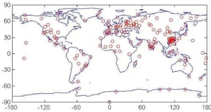
Figure 1. Global distribution of radiosounding sites used in CLAR.
θ. Finallyεand1εare the mean emissivity and emissivity difference for either the channels or the observation angles. 2.2 CLAR Database
The CLAR database was constructed with atmospheric radiosoundings taken from the Atmospheric Science De-partment, University of Wyoming (http://weather.uwyo.edu/ upperair/sounding.html). It contains 382 uniformly dis-tributed global land atmospheric radio-soundings. All of them were checked to ensure that no cloud was included. A radiosounding was considered cloudy when the relativity hu-midity (RH) of one layer was more than 90% or when two consecutive layers had H>85%. A radiosounding with a RH higher than 80% in the two first layers was considered a foggy radiosounding and was therefore rejected.
CLAR has a good distribution in W which is uniform until 5.5 cm and reach the 7 cm. The distribution of abso-lute latitude is based on three latitude ranges: 40% in low latitudes (0◦- 30◦), 40% in middle latitudes (30◦- 60◦), and 20% in high latitudes (>60◦). Figure 1 shows the global distribution of all the radiosounding stations used in CLAR. 2.3 Simulation characteristics
Since the atmospheric coefficients,ak, are independent
of emissivity, they can be derived from simulations for a black body surface. In which case the relationship between radiation measured for the channeli of the sensor atθ an-gle from nadir, Li, and the radiance emitted by the surface, Bi(T), obtained from the Planck function is as follows:
Li =τi(θ )Bi+L↑i(θ ) (2)
whereτi(θ )andL↑i(θ )are the atmospheric transmittance and
upward atmospheric radiance, respectively, which are calcu-lated for each atmospheric profile of the database with the radiative transfer model MODTRAN 4 (Berk et al., 1999). ThenTi is obtained from the radiance measured by the
sen-sor,Li, according toBi(Ti)=Li.
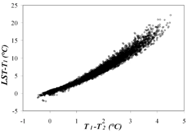
Figure 2.LST-T1 plotted in front of T1-T2 for the MSW case.
Figure 3.α(grey circle) andβ(black cross) coefficients for MSW algorithm in front of path water vapor contentW(cm).
was taken around the temperature of the first layer, T0. We selected seven temperatures: T0−6 K,T0−2 K,T0+1 K, T0+3 K,T0+5 K,T0+8 K andT0+12 K. Several observa-tion angles were considered, 11.6◦, 26.1◦, 40.3◦and 53.7◦, which are the so-called Gaussian angles. We also included two observation angles (0◦and 65◦) for completeness. Thus we achieved 16044 simulations to be used in obtaining the LST algorithms.
3 Algorithms
3.1 Algorithms generated
ASWn was generated from simulations obtained for the following observation angles: 0◦, 11.6◦ and 26.1◦. ASWf was generated from simulations only at 53.7◦. Simulations at two couples of observation angles, 0◦- 53.7◦and 11.6◦ - 53.7◦, were used for generating the two DA algorithms in the AATSR channels at 11 and 12µm.
Although the MODIS field of view can reach up to 65◦, we restricted ourselves toθ <45◦ in this paper. The reason is that there is little information about the angular variability of the emissivity and because of the degradation of regression results when angles larger than 45◦are used. Consequently, the MSW was generated using simulations obtained at 0◦, 11.6◦, 26.1◦and 40.3◦.
In the ASWn and MSW algorithms the coefficients α andβ were parameterizated as a function of the path water vapor content, cos(θ )W , because in those cases there was a larger variability of observation angles. For instance, in the case of MSW, Figure 2 shows the differences inL ST −T1 versus the brightness temperature differencesT1−T2. The relationship between theα andβ coefficients and the path water vapor content are shown in Figure 3. Similar results were obtained in the other algorithms. The algorithms can then be expressed as follows:
ASWn:
L ST =T11n+0.32(T11n−T12n)2+0.78(T11n−T12n) +0.24+(52.57+1.13cos(θ )W −1.023(cos(θ )W )2)(1−ε)
−(79.2−11.06cos(θ )W )1ε
(3)
ASWF:
L ST =T11f +0.437(T11f −T12f)2+0.49(T11f −T12f) +0.16+(55.2−4.4W −0.7W2)(1−ε)
−(64.6−11.432W)1ε
(4)
ADA11:
L ST =T11n+0.176(T11n−T11f)2+1.569(T11n−T11f) −0.059+(57.00+1.57W−1.18W2)(1−ε)
−(111.6−17.62W)1ε
(5)
ADA12:
L ST =T12n+0.303(T12n−T12f)2+1.57(T12n−T12f) −0.01+(64.5−4.53W−0.71W2)(1−ε)
−(110.3−19.84W)1ε
(6)
MSW:
L ST =T31+0.494(T31−T32)2+2.370(T31−T32)
+0.319+(45.99+4.67cos(θ )W −1.446(cos(θ )W )2)(1−ε)
−(160.5−25.75cos(θ )W )1ε
(7)
In the case of AATSR algorithms,T11nandT12nare the
brightness temperatures in nadir view in channels in 11µm and 12µm respectively, and T11f andT12f are the
bright-ness temperatures for the same channels but in forward view. Moreover, in the MSW algorithmT31andT32are the bright-ness temperature in bands 31 and 32, respectively.
3.2 AATSR and MODIS LST Operational Algorithms
Table 1. Emissivities used for the application of the algorithms in the Valencia test site.
ASWn ASWf ADA11 ADA12 MSW
ε 0.983 0.973 0.980 0.975 0.984
1ε 0.005 0.005 0.010 0.010 -0.003
fractional vegetation cover (f), the precipitable water and the satellite viewing angle.
These coefficients are provided for 14 different land cover classes. For a given land cover class, two separated sets of coefficients are given for the fully vegetated surface and for the bare surface. LST data generated with this al-gorithm are currently provided as a product with AATSR L2 data. The algorithm is operationally implemented at the Rutherford Appleton Laboratory (RAL) in the so-called RAL processor. The values of land cover class, fractional veg-etation cover, and precipitable water are taken from global classification, fractional vegetation cover monthly maps and global monthly climatology at a spatial resolution of 0.5◦×
0.5◦longitude/latitude.
The generalized split-window algorithm applied to the MODIS is expressed as a linear combination of the bright-ness temperatures. Theoretical expressions are given in Wan and Dozier (1996). Coefficients were obtained from linear regression of MODIS simulated data for wide ranges of sur-face and atmospheric conditions and depend on the view an-gle, W, and the atmospheric lower layer temperature. The emissivities required were obtained from pixel-classification-based emissivities (Snyder et al., 1998). LST data generated with this algorithm are currently provided as a product with MOD11 data.
4 Validation
The validation of satellite-derived LSTs with ground measurements is a challenging problem because of the heterogeneity of land surfaces both in temperature and emis-sivity. Only a few LST validation studies can be found in the literature (e.g., Prata, 1994; Wan et al., 2002; Coll et al., 2005 and 2006; Hook et al., 2007). The comparison between ground, point measurements and satellite, area-averaged measurements is only possible for certain land surfaces that are thermally homogeneous at various spatial scales, from the footprint of ground instruments to several satellite pixels. Such areas exist, the most suitable being inland waters or densely vegetated surfaces.
A database of LST ground measurements was collected concurrently with AATSR and MODIS overpasses in the summers of 2002-2006. This is a flat area of rice crops located close to Valencia, Spain. Every summer, this area has full cover vegetation and is well irrigated, which makes this site thermally homogeneous. This validation database
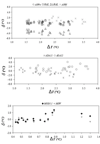
Figure 4.Algorithm errorδT as a function of the brightness tem-perature difference1T in Valencia site.
has been used to evaluate SW and DA correction methods (Coll et al., 2005 and 2006).
Nadir emissivity was measured in the field using the box method (Rubio et al., 2003). Off-nadir measurements were not available for the rice crops. The angular emissivity might be expected to be small in this case. For full cover crops and well-irrigated crops, the differences between nadir and off-nadir (60◦) brightness temperatures were within 0.5 K (Lagouarde et al., 1995). A temperature decrease of 0.5 K between nadir and off-nadir observations is approximately equivalent to an emissivity decrease of 0.01 between both viewing conditions. Table 1 gives the mean emissivity and emissivity differences used in all algorithms.
Table 2. LST algorithm errors obtained in the Valencia site (δT = average error;σ(T) standard deviation).
Number of Algorithm δT (K) σ(T) (K) RMSE (K) points
25 ASWn 0.0 0.5 ±0.5
25 ASWf 0.5 0.8 ±0.9
25 ADA11 -1.0 1.1 ±1.5
25 ADA12 -2.4 1.6 ±2.8
25 RAL1 -3.5 0.6 ±3.6
25 RAL2 -0.1 0.5 ±0.5
18 MSW 0.1 0.5 ±0.5
18 MOD11 0.1 0.6 ±0.6
The RAL processor classifies this site as broadleaf trees with groundcover (i = 6) and f = 0.40 0.47 (July -August). The value assigned to f seems very low for rice crops during summer. In fact, with these considerations the RAL processor appears to overestimate the ground LSTs by an average of 3.6 K (see Figure 4). The most accurate results for the AATSR LST algorithm were obtained in the class broadleaf shrubs with groundcover (i = 8) and f = 1 (full cover) referred to as RAL2 in Figure 4 and Table 2.
5 Conclusions
A new CLAR database was compiled to obtain LST algorithms for both techniques, SW and DA. By using this database and applying the method of Coll and Caselles (1997), LST algorithms for two sensors (AATSR and MODIS) were generated. Validation provided the error of the algorithms. Results of these algorithms were also compared to those provided by the AATSR and MODIS LST operational algorithms.
The most accurate results in the Valencia site were obtained using the SW algorithm with the exception of ASWf. The error is usually around±0.5 K, but in the case of ASWf it was approximately ±1.0 K. The low accuracy of the DA method is due to the directional effects in radio-metric temperatures expected for rough, nonisothermal land surfaces, and to uncertainties in the angular variation of land surface emissivity. In fact, these algorithms have an error of around±2.0 K. The accuracy of the DA algorithm decreases with the increase of roughness and thermal heterogeneity of the land surface.
Although the validation database has a few points and corresponds to only one site, the results show that SW algorithms can obtain the LST with a precision higher than
±1 K. In future research, there will be more sites to increase the validation database. The LST operational algorithm for MODIS is consistent with the SW algorithms proposed in the present paper. In the case of AATSR, the incorrect classification of the site caused errors much higher than expected.
Acknowledgements. We would like to thank the Department of Atmospheric Science, University of Wyoming for the atmospheric
radiosoundings profiles. This research was financed by the Min-isterio de Educaci´on y Ciencia (project CGL2004-06099-C03-01, cofinanced with European Union FEDER funds, acciones com-plementarias CGL2005-24207-E and CGL2006-27067-E, research contract of R. Nicl`os and the two research grants of J.M. Galve and Maria Mira), and the University of Valencia (V Segles research grant of J.M. S´anchez). We would like to thank the AATSR Valida-tion Team, University of Leicester, European Space Agency (under CAT-1 project 3466) and EOS-NASA for providing the AATSR and MODIS data.
References
Becker, F. and Li, Z., 1990:Towards a local split-window method over land surfaces, Int J Remote Sens,11, 369–394.
Berk, A., Anderson, G. P., Acharya, P. K., Chetwynd, J. H., Bern-stein, L., Shettle, E. P., Matthew, M. W., and Adler-Golden, J. H., 1999: MODTRAN 4 users manual, report, Air Force Research Laboratory Space Vehicles Directorate, Hascom AFB, Mass. Caselles, V., Coll, C., Valor, E., and Rubio, E., 1997:Thermal band
selection for the PRISM instrument: 2. Analysis and comparison of existing atmospheric and emissivity correction methods for land surface temperature recovery, J Geophys Res,102, 19 611– 19 627.
Coll, C. and Caselles, V., 1997:A split-window algorithm for land surface temperature from Advance Very High Resolution Ra-diometer data: Validation and algorithm comparison, J Geophys Res,102, 16 697–16 713.
Coll, C., Caselles, V., Galve, J. M., Valor, E., Nicl`os, R., S´anchez, J. M., and Rivas, R., 2005: Ground measurements for the val-idation of land surface temperatures derived from AATSR and MODIS data, Remote Sens Environ,97, 288–300.
Coll, C., Caselles, V., Galve, J. M., Valor, E., Nicl`os, R., and S´anchez, J. M., 2006:Evaluation of split-window and dual-angle correction methods for land surface temperature retrieval from Envisat/AATSR data, J Geophys Res,111, 12 105.
Hook, S., Vaughan, R., Tonooka, H., and Schladow, S., 2007: Abso-lute radiometric in-flight validation of mid and thermal infrared data from ASTER and MODIS using the Lake Tahoe CA/NV, USA automated validation site, IEEE Trans Geosci Remote Sens,15, 1798–1807.
Lagouarde, J. P., Kerr, Y. H., and Brunet, Y., 1995:An experimental study of angular effects on surface temperature for various plant canopies and bare soils, Agric For Meteorol,77, 167–190. McMillin, L. M., 1975: Estimation of sea surface temperatures
from two infrared window measurements with different absorp-tion, J Geophys Res,80, 5113–5117.
Prata, A. J., 1994:Land surface temperatures derived from the Ad-vanced Very High Resolution Radiometer and the Along Track Scanning Radiometer: 2. Experimental results and validation of AVHRR algorithms, J Geophys Res,99, 13 025–13 058. Prata, A. J., 2000: Land surface temperature measurement from
space: AATSR algorithm theoretical basis document, technical report, CSIRO Atmospheric Research, Aspendale, Australia, 27 pp.
Rubio, E., Caselles, V., Coll, C., Valor, E., and Sospedra, F., 2003:
experimental set-up and new measurements, Int J Remote Sens,
24, 5379– 5390.
Snyder, W. C., Wan, Z., Zhang, Y., and Feng, Y. Z., 1998: Classifi-cation based emissivity for land surface temperature from space, Int J Remote Sens,19, 2753–2774.
Wan, Z. and Dozier, J., 1996:A generalized split-window algorithm for retrieving land surface temperature from space, IEEE Trans Geosci Remote Sens,34, 892–905.