Remote sensing in food production - A review

REVIEW ARTICLE

Remote sensing in food production – a review

1

Departamento de Ciências e Engenharia do Ambiente, Faculdade de Ciências e Tecnologia, Universidade Nova de Lisboa, Quinta da Torre, 2829-516 Caparica, Portugal

2

CICEGe, Departamento de Ciências da Terra, Faculdade de Ciências e Tecnologia, Universidade Nova de Lisboa, Quinta da Torre, 2829-516 Caparica, Portugal

Abstract

FAO’s most recent assessments indicate that, globally, in 2011–13, about one in eight people in the world are

likely to have suffered from chronic hunger, not having adequate food supplies for an active and healthy life. Food security crises are now caused, almost exclusively, by problems in access to food, not absolute food availability, but, monitoring agricultural production remains fundamental. Traditional ground-based systems of production estimation have many limitations which have restricted their use. However, remotely sensed satellite data offer timely, objective, economical, and synoptic information for crop monitoring. The objective of this paper is to review the contribution of remote sensing techniques in the classification, monitoring of crop phenology and condition and estimation of production.

Key words: Remote sensing, Food production, Crop monitoring

Introduction

Food security is one of the most essential factors for our physical wellbeing. In fact, it is a vital condition for a healthy and happy life. The Food and Agriculture Organization of the United Nations (FAO) defines a food-secured world as “a situation that exists when all people, at all times, have physical, social, and economic access to sufficient, safe, and nutritious food that meets their dietary needs and food preferences for an active

and healthy life” (FAO et al., 2013). Unfortunately,

at present, the situation, at a planetary scale, is of

food insecurity. FAO’s most recent estimates

appoint that about 12% of the world population, about 842 million people, in the period 2011-2013, have suffered from chronic hunger, that is, they did not have access to enough food (FAO et al., 2013). Although this figure is lower than the corresponding value for 2010-2012, which means a progress was obtained in the attempt to achieve

hunger reduction, overall it is still insufficient (FAO et al., 2013).

Food security is not a simple concept. It comprises both physical and economic access to food that meets nutritional necessities of human beings as well as their food preferences. Four food security dimensions are usually considered: availability, access, utilization and stability (Grote, 2014). All of them must be fulfilled simultaneously so that food security objectives are achieved (FAO et al., 2013). Food availability, the physical supply of food stocks, plays an essential role in food security, it fact it provides the base for food security.

Food availability in any location depends on production, storage and transport infrastructures. Thus, food production is a key determinant of food availability and consequently of food security. In fact, in order to develop robust policies and strategies for food management that may guarantee food security, timely and accurate evaluations of global crop production are vital (Becker-Reshef et al., 2010).

Crop production depends on many factors, some intrinsic to the species being cultivated some extrinsic. Intrinsic factors refer to the biological lifecycle of crops which influence the seasonal patterns they may depict (Atzberger, 2013). Production depends, on other hand, on the physical characteristics of the land being cultivated, climatic

Received 1 June 2014; Revised 15 July 2014; Accepted 25 July 2014; Published Online 1 February 2015

*Corresponding Authors Maria Fernanda Pessoa

CICEGe, Departamento de Ciências da Terra, Faculdade de Ciências e Tecnologia, Universidade Nova de Lisboa, Quinta da Torre, 2829-516 Caparica, Portugal

factors and also on agricultural management practices (Atzberger, 2013). Information on crop development obtained as early as possible during the growing season is essential for an estimation of the probability of seasonal production deficits, which is especially important for food-insecure countries. Thus, early warning monitoring systems which provide timely and easily interpretable information available to decision makers are needed (Meroni et al., 2014). However, productivity can change within short time periods, due to the fact that extrinsic factors that influence crop productivity are highly variable in space and time, especially weather conditions. This clearly challenges the implementation of an efficient and prompt monitoring system (Atzberger, 2013). As pointed out by the Food and Agriculture Organization, information is worth little if it becomes accessible too late (FAO et al., 2013).

For the quantification of food production information on cultivated area, growth, status and yield of crops is needed.

Technologies, tools and methodologies for vegetation monitoring

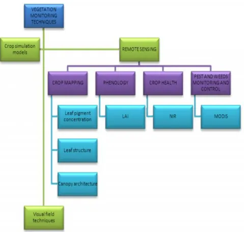
A range of techniques have been developed to estimate crop production with varying degrees of success (Becker-Reshef et al., 2010). They include visual field techniques, crop simulation models and remote sensing (Wall et al., 2007 in Becker-Reshef et al., 2010).

Crop yield monitoring with field techniques usually involves a first phase in which vegetation amount and condition are assessed during manual field sampling and a second phase in which the values obtained are processed and aggregated in order to produce a regional yield value. However, these methods are inadequate for large areas because they have high operating costs and are time-consuming and have thus been progressively abandoned (Wang et al., 2013).

Crop growth models simulate biogeophysical processes in crops systems, considering soil-crop-atmospheric interactions. They provide estimates of growth over time as well as the final yield. Crop simulation models use a variety of input data like climate information, soil type, plant varieties and management practices to forecast yield. They also include adjustments derived from disease, insect, and harvest losses (Moen et al., 1994 in Wang et al., 2013). Crop growth models have some important limitations: they are simplifications of reality and are also restricted by uncertainties in the input parameters (Fang et al., 2008 in Wang et al., 2013). Moreover, implementation at a large scale of

crop simulation models is limited by input data availability (Chipnashi et al., 1999 in Wang et al., 2013).

A more realistic approach is the use of remote sensing, which consists in the acquisition of information about objects or phenomenons without making physical contact, using, in general, aerial sensor technologies. Remote sensing has the ability to provide timely, synoptic, reliable information over a long time-period with high revisit frequency and with an excellent cost/benefit ratio, a fraction of the cost of traditional approaches (Manjunath et al., 2002; Lobell et al., 2003; Prasad et al., 2006; Nellis et al., 2009; Calvão and Palmeirim, 2011; Atzberger, 2013; Meroni et al., 2014). Moreover, remote sensing allows the acquisition of data in areas difficult to reach and at different resolutions (Wang et al., 2013). And in fact, agricultural monitoring from space has long been extensively utilized (as early as the 1930s) over a wide range of geographic locations and spatial scales (Wall et al., 2008; Nellis et al., 2009; Becker-Reshef et al., 2010; Atzberger, 2013; Piou et al., 2013).

Basis of remote sensing approach

Remote sensing techniques try to infer characteristics of objects from changes occurred in the properties of electromagnetic energy resulting from interactions with these objects. All bodies of the earth's surface reflect radiation from the sun and emit themselves energy. The intensity and spectral composition of the reflected/emitted radiation depend on the physical and chemical inherent properties of the objects. Moreover, the signal reaching sensors is influenced by external factors like the atmosphere and the geometry sun-object-sensor. The interpretation of remote sensing data requires the knowledge of the spectral properties of the different constituents of the Earth's surface as well as their variation caused by external factors. The spectral characteristics of the different plant species must be known for accurate estimation of biophysical parameters such as biomass and productivity from remote sensing methods (Camacho-De Coca et al., 2004).

The reflectance values of any object in the different regions of the electromagnetic spectrum allow the delineation of the spectral reflectance curve or spectral signature of that object. Green vegetation has a unique and complex spectral signature as compared to other materials on Earth (Camacho-De Coca et al., 2004). Compared with plants, the spectral signatures of bare soils, exposed rocks and sand, which constitute background for vegetation, are relatively simple (Hoffer, 1978;

Curran, 1983; Goward et al., 1985). These materials usually exhibit monotonic increases in reflectance throughout the visible and NIR regions (Satterwhite and Henley, 1987; Richards, 1993; Pinter et al., 2003). In the SWIR their spectra display more features than those observed in shorter wavelengths but are still much less complex than those of vegetation (Hoffer 1978; Curran 1983; Goward et al., 1985; Tucker and Sellers 1986; Pinter et al., 2003).

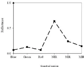
Plants have, in general, a complex structure, consisting of several leaf layers arranged according to various geometries and also of elements other than leaves, especially trunks and branches (Curran, 1983). The interactions between solar radiation and plant canopies are extremely complex and determine the amount of radiant energy that is absorbed, reflected or transmitted by plants and therefore the fraction available to the processes of photosynthesis and evapotranspiration. The spectral behavior of plant canopies depends, on one hand, on the canopy elements and, on the other hand, on their spatial organization (Homolová et al., 2013). However, vegetation spectral behavior is predominantly a function of the spectral properties of the leaves (Daughtry and Walthall, 1998). Green leaves typically display very low reflectance in the visible regions of the spectrum (0.4-0.7 µm), especially in the blue and red bands, a high reflectance in the near-infrared (0.7-1.3 µm), much greater than in any portion of the visible, and a variable reflectance in the middle infrared regions (1.3-2.5 µm) (Hoffer, 1978; Curran, 1983; Hardisky et al., 1983; Schneider, 1984; Goward et al., 1985, 1987; Milton and Mouat, 1989). The dominant factor controlling vegetation reflectance varies depending on the spectral region. Photosynthetic pigments are of fundamental importance in the response of vegetation in the visible spectral region. However, in the near infrared, this role is due essentially to the internal structure of the leaves. High reflectance in the near infrared is due to multiple scattering of light at the air-cell interfaces in the spongy mesophyll cells located in the interior or back of leaves. In the mid-infrared spectral region the vegetation behavior is mainly determined by the water content of the leaf tissues (Sinclair et al, 1971; Hoffer, 1978; Barrett and Curtis, 1982; Boyer et al., 1988).

Vegetation typically shows a large difference between the values of the spectral reflectance in the red and near infrared regions (low red reflectance and high reflectance in the near infrared) (Figure 1). It has been found that as canopy green area

increases, either due to increasing crop density or photosynthetic pigments content this difference also increases (Schneider et al., 1985; Scotford and Miller, 2005). Rather, the substrate component has usually a more attenuated difference between the reflectance values in these two regions (Tucker and Sellers, 1986; Bartlett et al., 1988; Scotford and Miller, 2005). It is comprehensible, therefore, that many studies of vegetation using remote sensing data use the spectral regions of the red and near infrared (Pinter et al., 2003). In the spectral signature of green leaves there is a sharp increase in reflectance values in the transition zone from the visible to the near infrared region, between about 0.7 and 0.75 µm (Hoffer, 1978; Boyer et al., 1988). This abrupt variation in reflectance is generally

referred to as the ``red edge” and is due to a change

of processes: from the absorption of visible light by photosynthetic pigments to the diffusion of near infrared radiation in the internal structure of the leaves. Research has documented that measures based on the red edge position or shape are well correlated with canopy biophysical parameters. However, they are less influenced by atmospheric effects and background noise (Mauser and Bach, 1995 in Broge and Leblanc, 2000). For example, it has been found that due to situations of nutrients deficiency this inflection point of the spectral curve can oscillate towards higher or lower wavelengths (Boyer et al., 1988).

Figure 1. Spectral behavior of a healthy leaf.

Methods of vegetation monitoring using remote sensing data

In a remote sensing-based approach two main types of methods have been developed to estimate vegetation quantity and condition. One type consists in the development of physiology-based

plant growth models and the other type in the development of empirical or semi-empirical relationships between plant biophysical parameters and arithmetic combinations of reflectance from different spectral bands into a single metric.

Physiology-based plant growth models simulate biophysical processes and compute crop growth in the different stages of plant development, from emergence till maturity. Their main drawback is that they typically need numerous inputs that are specific to the crop species, soil type, management practices and local environmental conditions (Doralswamy et al., 2003; Becker-Reshef et al., 2010). Some of the inputs are remotely-sensed driven variables such as weather related events that affect plant development (Doralswamy et al., 2003; Howard et al., 2012). Due to the lack of available data these models have had limited application at scales larger than field scale (Doralswamy et al., 2003). Prasad et al. (2006) developed a model for crop yield assessment for corn and soybean using NDVI from the AVHRR, soil moisture, surface temperature and rainfall, for the state of Iowa (US Corn Belt). The model developed showed promising results for forecasting crop yields at regional and global scales.

The other type of methods for vegetation characterization through remote sensing involves the development of empirical or semi-empirical relationships between plant biophysical parameters and arithmetic combinations of reflectance from different spectral bands into a single metric, the so

called “vegetation indices” or VIs (Tucker, 1979;

Pinter et al., 2003). VIs have been found to be related to a number of vegetation biophysical parameters such as biomass, Leaf Area Index (LAI, the total one-sided area of photosynthetic tissue per unit of ground surface area) percent vegetation cover, fraction of absorbed photosynthetically active radiation and crop yield (Baret and Guyot, 1991; Liu and Huete, 1995; Hurcom and Harrison, 1998; Gitelson, 2004). A major weakness of VIs is that relationships are often site specific and thus their extrapolation to new areas is not always feasible or recommended (Becker-Reshef et al., 2010). However, compared to simulation models advantages of VIs consist on their simplicity of implementation, transparency and limited data requirements (Becker-Reshef et al., 2010). And, in fact, since the early 80s, satellite imagery-based spectral VIs have been extensively used and constitute an important tool in the mapping and monitoring of terrestrial ecosystems because they are well correlated with green biomass and leaf area index of crop canopies (Pinter et al., 2003). They

provide key measurements in productivity, phenology, vegetation health and biodiversity studies (Prasad et al., 2006).

The rationale for VIs lies on the fact that green vegetation has a unique and complex spectral behavior as compared to other materials on Earth (Huete et al., 1994; Camacho-De Coca et al., 2004). Different VIs based on the combination of two or more spectral bands have been developed as it has been found that multi-band combinations are more sensitive to changes in vegetation amount and state than information from single bands (Liu and Huete, 1995; Rondeaux et al., 1996; Henry and Hope, 1998; Schmidt and Karnieli, 2001). Each VI has its specific advantages and limitations. VIs is sensitive to external influences such as the presence of background, atmospheric effects and illumination geometry (Rondeaux et al. 1996; Govaerts et al. 1999; Schmidt and Karnieli 2001). An ideal VI should be very sensitive to vegetation biophysical parameters and rather insensitive to these external perturbing factors (Calvão and Palmeirim, 2011). Soil-adjusted VIs such as the Soil Adjusted Vegetation Index (SAVI) and its various versions, known as the SAVI family, were developed in order to minimize brightness-related soil effects on VI performance, an important phenomenon, especially at low vegetation cover (Huete, 1988; Qi et al., 1994; Pinter et al., 2003). However, even these VIs are influenced, to some extent, by background (Broge and Leblanc, 2000).

Some other VIS was designed to minimize atmospheric influence like GEMI and ARVI. These are called atmospherically resistant vegetation indices (Kaufman and Tanre, 1992).

However, even if the influences of external factors could be completely removed, the type of VIs that use reflectance data from red and NIR bands would still have intrinsic limitations because they are not a single measure of a specific plant biophysical parameter but rather of many vegetation parameters (Govaerts et al., 1999; Haboudane et al., 2004). In fact, a major problem in the use of these VIs arises from the fact that canopy reflectance, in the visible and near infrared, strongly depends on both structural (LAI, leaf orientation, canopy architecture) and biochemical properties (e.g., photosynthetic pigments content) (Asner, 1998; Gao et al., 2000; Haboudane et al., 2004). It is difficult to uncouple the combined effect of the two influences (red and NIR spectral

regions) and, consequently, to develop a “unique”

VI exclusively sensitive to a single vegetation property, as Agapiou et al. (2012) point out. However, some authors have recently demonstrated

that chlorophyll concentration can be assessed with minimal confounding effects owing to LAI based on a combination of two types of spectral indices: indices sensitive to pigment content and indices resilient to background influence (Broge and Leblanc, 2000; Daughtry et al., 2000; Haboudane et al., 2004). Though, these VIs tend to use other spectral regions besides red and NIR regions.

The Normalized Difference Vegetation Index (NDVI) is one of the most widely used vegetation indices because it is of simple calculation, has a high degree of standardization and assumes no assumption about the distribution of the data (Curran, 1983). In the formulation of this index the difference between the values of reflectance in red and near infrared is normalized relative to the sum of these values, a fact that partially compensates changes in atmospheric conditions and solar irradiance (Curran, 1983; Hardisky et al., 1984; Tucker et al., 1985; Johnson, 2014). The normalization also allows for easier comparison of data from different sensors (Johnson, 2014). Some authors have found almost linear relation between NDVI and Leaf Area Index (LAI)/fAPAR (fraction of Absorbed Photosynthetically Active Radiation) (Prince, 1991 in Atzberger, 2013). However, other authors have demonstrated that its main weakness is the inherent nonlinear relationship it sometimes displays with many vegetation biophysical parameters, saturating at high levels of biomass. Besides, NDVI is extremely sensitive to the optical properties of background materials, especially at low vegetation cover (Broge and Leblanc, 2000; Schmidt and Karnieli, 2001). In spite of these disadvantages, NDVI, since it reflects vegetation greenness and thus indicates levels of healthiness in the vegetation development, has been widely used since the early 1980s, and is, at present, the only operational, global-based VI used for vegetation monitoring, crop yield assessment and forecasting (Roujean and Breon, 1995; Calvão and Palmeirim, 2011; Becker-Reshef et al., 2010).

The majority of VIs used in agricultural studies use the red and near infrared wavelengths (Scotford and Miller, 2005). However, others explore additional regions of the spectrum (Agapiou et al., 2012). VIs can be classified in different ways, the

simplest one refers to the wavelength

characteristics used in their formulation: broadband indices based on broadband spectral data and narrowband indices based on narrowband spectral data (hyperspectral, i.e., reflectance for many contiguous narrow wavelength bands). Landsat TM and SPOT sensors provide broadband multispectral

data. An example of a narrowband hyperspectral

spaceborne sensor is NASA’s Earth Observing-1

Mission Hyperion, capable of capturing high resolution images of the earth surface in 220 contiguous spectral bands (Manevski et al., 2011). Broad waveband VIs usually lack diagnostic ability for recognizing a particular biophysical characteristic and thus narrowband indices were developed. Hyperspectral VIs have been proposed to detect water, nutrient, and pest-induced stress in plants, at the same time minimizing unwanted influences (Pinter et al., 2003). However, the interpretation of the high quantity of data obtained from hyperspectral sensors can be complex due to the inter-dependency between wavelength (Scotford and Miller, 2005). Roberts et al. (2011) in Agapiou et al. (2012) refer that narrowband VIs can be divided into three main categories, according to the biophysical parameters being investigated: structure, biochemistry and plant physiology/stress.

Existing satellite systems used in agriculture monitoring

Due to the rapid development of remote sensing technology there has been an increase in the availability of remotely sensed images which can be acquired from a variety of platforms such as satellite, aircrafts, unmanned vehicles and handheld devices and gathered by different instruments like radiometers, film cameras, digital cameras, and video recorders. As regards agricultural monitoring satellites are of great importance. At present, data obtained from sensors onboard different satellites on many orbits provide a wide range of images which differ with respect to spectral, spatial, radiometric and temporal characteristics (Ahmed et al., 2011; Atzberger 2013).

As regards crop monitoring medium spatial resolution (10-100 m) images are the most the most frequently used at regional/national scale. This includes data from Landsat series satellites and SPOT (Ahmed et al., 2011). The advantages of using medium spatial resolution satellite imagery consist in the fact that, due to the resolution, large areas can be captured in a single image. Additionally, the medium temporal resolution of these satellites (around fortnightly) makes them suitable for many agricultural applications. However, for specific studies a timing window of sensing of only a few days is required as is the situation of the necessity to apply inputs at the correct time and the rapid development of the crop canopy that urges crop harvest (Ahmed et al., 2011). Ikonos and Quickbird satellite sensors have a high temporal observation frequency (<3 days).

On the other hand these sensor have high spatial resolution (<5m) which allows their use in detailed studies (Joyce et al., 2009).

Crop mapping

The first step in the prediction of crop production is the determination of the spatial distribution and areal extent of the different crops present in the rural landscape, that is, the assessment of crop identity. Then, cop production can be computed incorporating yield assessments per unit area which can be retrieved both from ground sampling and remote sensing data.

The classification of crops from remote sensing methods has become an important part of agricultural management (Van Niel and Mc Vicar, 2004). One of the most important applications of remote sensing consists in the classification of objects at the earth surface and, in fact, plant communities have been classified and mapped using a wide variety of remote sensors (Manevski et al., 2011). Crop classification is based on the differential spectral behavior of the various crops present in the study area (Xie et al., 2008). Spectral classes of the imagery are then converted into the different plant species in the interpretation process. For that purpose many methods have been developed that aim increasing classification accuracy (Van Niel and Mc Vicar, 2004). These classification methods include supervised and unsupervised methods. Supervised methods are time-consuming because they require human intervention, that is, classifiers have to be developed by hand. Thus, they are impractical for large area applications. For that reason unsupervised methods were developed which automatically generate classifiers and then maps of the crops in the study area (Yan and Roy, 2014).

In many cases a multi-temporal approach can be used to increase classification accuracy and, consequently, to enhance the mapping process efficiency, when single date information does not allow accurate crop discrimination (Van Niel and Mc Vicar, 2004; Xie et al., 2008). In fact, the spectral behavior of plants has a temporal aspect (Hoffer, 1978). As plants develop biomass increases, until maturity, there are changes in leaf pigment concentration and in leaf structure and canopy architecture. These temporal changes, known as phenology, affect the interaction between plant canopy and solar radiation, and their analysis can improve the accuracy of crop classification and thus crop yield estimation.

Phenology

Vegetation phenology is the study of the timing of seasonal developmental stages in plant life cycles which are closely coupled to seasonally varying weather patterns. These stages include budburst and swelling, vegetative growth, flowering, fruit setting and fruit maturing as well as senescence (Mounzer et al., 2008). The timing of phenological events is essential for efficient crop management since it allows growers to program management practices like planting and harvest times, fertilization application, irrigation and pest control (Mounzer et al., 2008).

The spectral behavior of plant canopies changes with stage of growth due to variations in leaf structure, water content and concentration of biochemicals, biomass, percentage of leaves, branches, flowers and fruits, and to differences in the architectural arrangement of the various canopy elements which results in the variation of background influence with time (Pinter et al., 2003). These facts allow the remote sensing of plant phenology. Vegetation reflectance is primarily a function of the optical properties of leaves, but also of other canopy elements (non-photosynthetic elements such as branches and trunks), canopy architecture (leaf and stem orientation, foliage clumping), background reflectance, illumination conditions, viewing geometry and atmospheric influence (Baret and Guyot, 1991; Asner, 1998; Huete et al., 1999; Gao et al., 2000; Homolová et al., 2013). Even when leaf spectral properties remain constant, the spectral signature of vegetation varies as the architectural arrangement of plant components changes and also the proportion of soil and plants (Pinter et al., 2003). Airborne sensors obtain an integrated view of all these effects, that is, the signal received from a single surface element (pixel) is presumed to be the contribution of different vegetation and bare soil components.

Canopy structure consists in the spatial arrangement of the different elements of a plant canopy and it decisively determines the interactions between solar radiation and vegetation. In fact, canopy structure impacts canopy reflectance by positioning the plant elements in the three-dimensional space and thus providing the chance for photons to interact with these elements as well as with background (Asner, 1998; Calvão and Palmeirim, 2011). Since plant architecture is influenced by a number of parameters and processes, not only intrinsic (ontogeny) but also extrinsic, like water availability, cultivation practices, pests and diseases, its changes over time

can provide important information on plant stage and condition. This means remote sensing can be a powerful tool for assessing crop state, drought severity, nutrients deficiency as well as monitoring diseases and pests.

Leaf area index (LAI) is the most widely used descriptor of canopy structure in remote sensing studies (Homolová et al., 2013). LAI refers to the amount of leaf material present in plant canopies and consequently controls various processes such as photosynthesis, respiration, transpiration and rain interception. LAI affects, in a decisive way, the

photosynthetically active radiation

absorbed/reflected by the canopy and, therefore, the energy balance of the plant. LAI is closely related to the total biomass of the plant. It is comprehensible, then, that monitoring LAI variation during the growing season is essential for assessing crop growth and vigor. LAI is also an important parameter not only for the estimation of primary production but also in land-surface processes and parameterizations in climate models (Nellis et al., 2009). LAI can be determined directly during field surveys by stripping off all the leaves and measuring their area but it can also be retrieved using remote sensing information. As the canopy of plants develops there is usually an increase in the number of canopy layers and leaves, a fact that will enhance NIR reflectance, mainly owing to the increase in the number of refractive index discontinuities inside leaf tissues. On the other hand, with an increase in leaf quantity, red reflectance decreases, due to increased absorption by photosynthetic pigments. Many authors (Wu, 2014) found good correlations between VIs and LAI. However, linear relationship between VIs and LAI only occurs between growth stages and canopy closure. After this situation, which varies depending on the crop species and variety (usually at a LAI of three), there is a saturation of the VI value, independently of LAI increase (Scotford and Miller, 2005).

Vegetation fraction is an important biophysical parameter, able to document ecological and environmental changes and thus relevant for agricultural and forestry studies, environmental management and land use. Fraction of vegetation cover is frequently an input for many models such as climate and soil erosion models. During crop development there is usually a gradual increase in crown cover and remote sensing can detect these changes. Gitelson et al. (2002) used spectral VIs to estimate cover fraction for wheat and corn.

When plants are at an early stage of development they have low biomass, LAI and canopy cover. Consequently, there is an important contribution from the bare soil that forms the background to the crop signal. As plants grow there is an increase in the values of these biophysical parameters which results in a reduction of red reflectance and an increase in NIR reflectance. Thus, as the growing season advances, the value of spectral VIs increases. At full growth the greatest rate of variation of the spectral reflectance from different plant species occurs as each species has developed its own canopy architecture and at the same time there is minimal influence of background. Each crop type has a characteristic spectral signature which permits its discrimination using remote sensing methods (Knipling, 1970). In maturity and senescence there is a decrease in NIR reflectance and an increase of red reflectance (Haboudane et al., 2004). Due to this fact vegetation spectral reflectance does not change meaningfully between different species. As the various crop species may take different time for full development, it is important to have data on crop state in a repetitive and updated form. Remote sensing offers, due to the possibility of multitemporal data collection, the opportunity to study the evolution of vegetation spectral signature over the growing season (each species has its own hallmark), to elaborate the temporal response curve for different VIs and thus of accompanying broad-scale crop phenology from space (Nellis et al., 2009). Therefore it provides invaluable guidance to farmers as regards crop harvest times and associated logistics like transportation and processing. In fact many crops need to be harvested without delay as they reach maturity, in order to provide the highest quality products, otherwise crop quality deteriorates quickly.

Crop health

For an efficient agricultural exploration it is essential to have timely and spatialized information on crop health and vigor, besides crop seasonal progress (Atzberger, 2013). In fact crop vigor and condition are early indicators of crop yield, crop risk and ultimately of the degree of crop success. Factors like diseases and pests affect a wide variety of crops worldwide and result in significant yield loss, which constitutes a serious limitation to any forecasting method (Prasad et al., 2006). Some authors report (Christou and Twyman, 2004; Strange and Scott, 2005) that at least 10% of the global food production is lost owing to plant diseases. Disease and pest control could become

more efficient if infected areas were identified as early and accurately as possible. For example, in many situations pesticides are applied excessively which not only causes potential risks to the agricultural products and the ecosystem but also increases the cost of production (Zhang et al., 2003). Diseases and pests have a dynamic nature which hinders their detection in a timely manner. Crop health monitoring can be undertaken using traditional ground-based sampling, however, these methods are labor intensive, have high costs and low efficiency, hence being impractical for large areas. In this context remote sensing has played an important role in agriculture monitoring by providing well-timed information on crop health and vigor over extensive areas with relatively low cost.

In order to identify modifications in plant condition by remote sensing approaches it is essential to be able to detect changes in the spectral behavior of plants (Pinter et al., 2003). Diseases and water and nutrients deficiency cause changes in photosynthetic pigments, internal structure of the leaves, foliar water and nutrient content. These changes affect canopy reflectance characteristics which can be detected by remote sensing (Raikes and Burpee 1998; Nellis et al., 2009). Because of the importance of leaves, variations in their condition may offer important information regarding the whole plant status. The reflectance curve of leaves in the visible spectral region, as earlier detailed, shows two minima: one in the blue region and the other in the red region, due to the intense absorption of sunlight by photosynthetic pigments, essentially by chlorophylls (Hoffer, 1978; Boyer et al, 1988). Besides, in the NIR spectral region healthy green vegetation is characterized by high reflectance values. Environmental stress conditions, diseases and normal end-of-season senescence typically result in yellowed or chlorotic leaves. These color changes are due to a decrease in the production of chlorophylls that then allow the expression of other photosynthetic pigments such as carotenoids (carotenes and xanthophylls). Chlorophylls tends to decline more rapidly than carotenoids when plants are under stress or during senescence (Sims and Gamon, 2002; Kopacková et al., 2014). Carotenoids have a single absorption peak in the blue region, their presence being normally masked by chlorophylls which also absorb radiation in the blue region. These chemical changes cause important variations in the spectral response of leaves. There is a noticeable increase in visible reflectance due to a reduction in the overall

absorption of visible light (there is a reduction in green reflection and an increase in red and blue reflections) and a broadening of the green reflectance peak towards longer wavelengths (Adams et al., 1999 in Pinter et al., 2003). When crops are affected by diseases and stressful conditions initial changes in the spectral behavior occur in the visible region because of the sensitivity of chlorophyll to physiological disturbances. There may be also a decrease in NIR reflectance, although proportionately less than the visible increase, due to changes of foliar internal structure (Knipling, 1970; Asner, 1998). These drastic changes in vegetation signatures impact VIs values of vegetation which are thus capable of indicating crop status as respects health and vigor. With increasing stress

conditions the “red edge” feature (the abrupt

transition normally present between visible and NIR reflectance values in the case of healthy green vegetation) moves towards shorter wavelengths and may even disappear in the case of senescent vegetation (Pinter et al., 2003).

Stress and disease often result in the loss of leaves or in their orientation. In this situation NIR reflectance decreases quickly due to a reduction in NIR enhancement of vegetation, owing to fewer multiple leaf layers and also because of an increase in background contribution (Knipling, 1970). Plant–soil interactions (which result in water or nutrient deficiency) may affect the chemical properties of leaves and structural properties of canopies, a fact that impacts decisively their spectral behavior (Carvalho et al., 2013).

All the changes resulting from the incidence of diseases of stress influence plant spectral behavior

and thus the value of spectral indices. In an “early warning” approach the VI value for the current

growing season for each crop species can be compared to the corresponding long-term value, which will indicate if environmental conditions are

more or less favorable compared to the “usual”

situation (Atzberger, 2013). Remote sensing thus enables precise diagnosis of crop stress, allowing timely remedial action.

Pests and weeds monitoring and control

Weeds can significantly reduce crop yield if not controlled. Clarke et al. (2000) in Scotford and Miller (2005) report that a reduction of winter wheat yields by 50% can happen due to weed competition, a fact that understandably results in high economic damages. The temporal aspect is particularly important in weed control as the application of treatments, for the best efficiency, should take place on a well-defined and restricted

period of time. In order to select the best type and quantity of herbicide, the weed needs first to be identified and its growth stage and density determined (Scotford and Miller, 2005). In general the most common arrangement of weeds in crop fields is the patchy or aggregated distribution (Felton, 1995 in Scotford and Miller, 2005), which impedes their timely detection using ground sampling methods. However, remote sensing techniques can be used for weed identification and localization. Biller (1998) in Scotford and Miller (2005) refers an herbicide reduction amount of 30 to 70% in the context of a system based on optoelectronic sensors to identify the weed plants, as compared with conventional treatments and still reported 100% weed control.

Since ancient times locust plagues have had a negative impact on food security in vast arid and semiarid regions of the world (Ji et al., 2004, Zhenbo et al., 2008). While the outbreaks alone are not responsible for famines, they can be an important contributing factor. Clouds of locusts have had tragic consequences in many countries, with incalculable destruction of crops and natural vegetation. Although in some areas control measures have eliminated locust plagues in the 20th century, they have become a serious problem again in recent decades, the frequency and severity of the damages caused being greater than before (Ji et al, 2004).

There are three forms in the life of these insects: the egg form, the solitary form and the gregarious form. The solitary form is wingless and does not constitute a threat (Piou et al., 2013). In this form individuals seem to avoid one another and constitute low density populations (Sword et al., 2010). However, due to favorable conditions, local population size increases which results in close contact among individuals. This triggers the shift from the harmless solitarious form to the gregarious winged sexually mature form (van Huis, 1995; Sword et al., 2010). Then the insects reproduce and develop quickly, as Ji et al. (2004) report, forming vast swarms that have the ability to fly rapidly across great distances and which, if not detected and controlled in time, can have catastrophic effects on agricultural production (Hielkema et al. 1986; Piou et al., 2013). The transition from the solitary to the gregarious phase is triggered by the occurrence of favorable ecological conditions caused by heavy rains able to provide enough moisture for egg hatching and also for the growth of vegetation that will make available food and shelter for the grasshoppers (van Huis, 1995).

These insects, with high reproductive potential, then multiply rapidly, in an exponential way, forming numerous swarms that coalesce (Piou et al., 2013). They leave their original area looking for food and may reach distant territories (Tucker et al., 1985). Thus, locust plague monitoring and control are of international concern in order to guarantee food security, given the catastrophic impacts of outbreaks (Ji et al., 2004; Zhenbo et al., 2008). Locust control should occur before the onset of the gregarious phase or as soon as insects start changing from the solitarious to the gregarious phase, when insects still occur in small numbered populations in reduced patches of favorable habitat (Piou et al., 2013). In fact, the strategy for the prevention of outbreaks occurrence is based on the location of possible areas with ecological conditions conducive to the rapid development of the insect and application of control measures in those areas, such as the application of insecticides, while populations still have low density and animals are wingless.

It is, therefore, essential to efficiently detect areas where locusts form changes, known as outbreak or recession areas as early as possible. However, this may become a challenging task due to the fact that the recession areas of the species are very large (Hielkema et al., 1986; Ji et al., 2004; Piou et al., 2013) and also because in those areas rainfall is highly unpredictable. In fact, it is very difficult and expensive, by traditional methods alone, based on ground-based surveys, to gather timely data of sufficient quality to accurately evaluate locust population dynamics in order to decide the optimum period for the application of control measures (Showler, 2002; Ji et al., 2004; Piou et al., 2013). An alternative to traditional techniques is the use of satellite imagery. Locusts cannot be identified directly with satellite images due to their tiny size. However, the remote sensing approach allows, over a large geographic scale, the identification and monitoring of the ideal conditions for the occurrence of outbreaks, that is, an increase, to a key value, of soil moisture and green vegetation (Ji et al., 2004; Zhenbo et al., 2008; Piou et al., 2013). On the other hand, remote sensing techniques allow quick damage assessment, comprising both the identification of the areal extent and the severity of losses (Ji et al., 2004). Since the late 1970s, remote sensing techniques have been used to detect potential outbreaks in different areas (Tucker et al., 1985; Hielkema et al., 1986; Ji et al., 2004). This approach has effectively allowed the early reduction of swarms, thus

preserving crops that would have otherwise been lost (Zhenbo et al., 2008). Hielkema et al. (1986) found good correlations between AVHRR NDVI values indicating potential breeding areas and locust population density in northwest Africa. Zhenbo et al. (2008) successfully used MODIS imagery to detect soil humidity in different areas in China and related moisture values to locust outbreaks. Also in China Ji et al. (2004) assessed locust damage using NDVI derived from the MODIS data. Their results showed that this VI reliably distinguished between before outbreak conditions and during outbreak destruction conditions for different categories of damage. However, authors like Tratalos and Cheke (2006) in Piou et al. (2013) refer that NDVI data at coarse resolution are not a good predictor of locust presence.

Figure 2 summarizes the three main techniques used on vegetation monitoring, especially based on remote sensing possibilities.

Conclusions

Timely and accurate estimates of crop production are crucial in order to develop well-timed and robust policies and strategies for food management that may guarantee food security. Traditional methods of obtaining this information consists in census and ground surveys which have the disadvantages of being time consuming and expensive. However, the use of remote sensing has proved to be very important in the monitoring and estimation not only of crop yield but also of crop condition and state.

Author Contributions

T. C designed the study. T. C. and F. P. wrote the article and corrected it. Figure 1 is from T. C. and Figure 2 is from F. P.

References

Agapiou, A., D. G. Hadjimitsis and D. A. Alexakis.

2012. Evaluation of broadband and

narrowband vegetation indices for the identification of archaeological crop marks. Remote Sens. 4:3892-3919.

Ahamed, T., L. Tian, Y. Zhabg and K. C. Ting. 2011. A review of remote sensing methods for biomass feedstock production. Biomass Bioener. 35:2455-2469.

Asner, G. P. 1998. Biophysical and biochemical sources of variability in canopy reflectance. Remote Sens. Env. 64:234–253.

Atzberger, C. 2013. Advances in remote sensing of agriculture: context description, existing operational monitoring systems and major information needs. Remote Sens. 5:949-981. Baret, F. and G. Guyot. 1991. Potentials and limits

of vegetation indices for LAI and APAR assessment. Remote Sen. Env. 35:161-173. Barrett, E. C. and L. F. Curtis. 1982. Introduction to

environmental remote sensing. Chapman and Hall, Ltd., London. p.52.

Bartlett, D. S., M. A. Hardisky, R. W. Johnson, M. F. Gross, V. Klemas and J. M. Hartman. 1988. Continental scale variability in vegetation reflectance and its relationship to canopy morphology. Int. J. Remote Sens. 9:1223-1241.

Becker-Reshef, I., E. Vermote, M. Lindeman and C. Justice. 2010. A generalized regression-based model for forecasting winter wheat yields in Kansas and Ukraine using MODIS data. Remote Sens. Env. 114:1312–1323. Boyer, M., J. Miller, M. Belanger and E. Hare.

1988. Senescence and spectral reflectance in leaves of Northern Pin Oak (Quercus palustris Muenchh.). Remote Sens. Env. 25:71-87. Broge, N. H. and E. Leblanc. 2000. Comparing

prediction power and stability of broadband and hyperspectral vegetation indices for estimation of green leaf area index and canopy chlorophyll density. Remote Sens. Env. 76:156–172.

Calvão, T. and J. M. Palmeirim. 2011. A comparative evaluation of spectral vegetation indices for the estimation of biophysical characteristics of Mediterranean semi-deciduous shrub communities. Int. J. of

Remote Sens. 32:2275-2296.

Camacho-De Coca, F., F. J. García-Haro, M. A. Gilabert and J. Mélia. 2004. Vegetation cover seasonal changes assessment from TM imagery in a semi-arid landscape. Int. J. Remote Sens. 25:3451–3476.

Carvalho, S., M. Schlerf, W. van der Putten and A. K. Skidmore. 2013. Hyperspectral reflectance of leaves and flowers of an outbreak species discriminates season and successional stage of vegetation. Int. J. App. Earth Observ. Geoinfor. 24:32–41.

Christou, P. and R. M. Twyman. 2004. The potential of genetically enhanced plants to address food insecurity. Nutri. Res. Rev. 17:23–42.

Curran, P. J. 1983. Problems in the remote sensing

of vegetation canopies for biomass

estimation. In: R. Fuller (Ed.), pp. 84-100, Ecological mapping from ground air and space, Institute of Terrestrial Ecology, NERC. Daughtry, C. S. T. and C. L. Walthall. 1998.

Spectral discrimination of Cannabis sativa L. leaves and canopies. Remote Sens. Env. 64:192-201.

Daughtry, C. S. T., C. L. Walthall, M. S. Kim, E. Brown de Colstoun and J. E. McMurtrey. 2000. Estimating corn leaf chlorophyll concentration from leaf and canopy reflectance. Remote Sens. Env. 74:229–239. Doraiswamy, P. C., S. Moulin, S., P. W. Cook and

A. Stern. 2003. Crop Yield Assessment from Remote Sensing. Photogram. Engine. Remote Sens. 69:665–674.

FAO, IFAD and WFP. 2013. The State of Food Insecurity in the World. The multiple dimensions of food security. Rome, FAO. Gao, X., A. R. Huete, W. Ni and T. Miura. 2000.

Optical-biophysical relationships of vegetation spectra without background contamination. Remote Sens. Env. 74:609–620.

Gitelson, A. A. 2004. Wide dynamic range vegetation index for remote quantification of biophysical characteristics of vegetation. J. Plant Physiol. 161:165–173.

Gitelson, A., Y. Kaufman, R. Stark and D. Rundquist. 2002. Novel algorithms for remote estimation of vegetation fraction. Remote

Sens. Env. 80:76–87.

Govaerts, Y., M. M. Verstraete, B. Pinty and N. Gobron. 1999. Designing optimal spectral indices: a feasibility and proof of concept study. Int. J. Remote Sens. 20:1853-1873. Goward, S. N., C. J. Tucker and D. G. Dye. 1985.

North American vegetation patterns observed with the NOAA-7 Advanced Very High Resolution Radiometer. Vegetatio. 64:3-14. Goward, S. N., D. Dye, A. Kerber and V. Kalb.

1987. Comparison of North and South American biomes from AVHRR observations. Geocarto Internat. 1:27-39.

Grote, U. 2014. Can we improve global food security? A socio-economic and political perspective. Food Sec. 6:187–200.

Haboudane. D., J. R. Miller, E. Pattey, P. J. Zarco-Tejada and I. B. Strachan. 2004. Hyperspectral vegetation indices and novel algorithms for predicting green LAI of crop canopies: Modeling and validation in the context of precision agriculture. Remote Sens. Env. 90:337–352.

Hardisky, M. A., R. M. Smart and V. Klemas. 1983. Seasonal spectral characteristics and aboveground biomass of the tidal marsh plant, Spartina alterniflora. Photogram. Engine. Remote Sens. 49:85-92.

Hardisky, M. A., F. C. Daiber, C. T. Roman and V. Klemas. 1984. Remote sensing of biomass and annual net aerial primary productivity of a salt marsh. Remote Sens. Env. 16:91-106.

Henry, M.C. and A. S. Hope. 1998. Monitoring post-burn recovery of chaparral vegetation in southern California using multi-temporal satellite data. Internat. J. Remote Sens. 19:3097–3107.

Hielkema, J. U., J. Roffey and C. J. Tucker. 1986. Assessment of ecological conditions associated with the 1980/81 desert locust plague upsurge in West Africa using environmental satellite data. Int. J. Remote Sens. 7:1609-1622.

Hoffer, R. M. 1978. Biological and physical considerations in applying computer-aided analysis techniques to remote sensor data. In: P. H. Swain and S. M. Davis (Eds.), pp. 227-289. Remote sensing: the quantitative approach, edited by Mc Graw-Hill Book Company.

Homolová, L., Z. Malenovský, J. G. P. W. Clevers, G. García-Santos and M. E. Schaepman. 2013. Review of optical-based remote sensing for plant trait mapping. Ecol.l Complex. 15:1–16. Howard, D. M., B. K. Wylie and L. L. Tieszen.

2012. Crop classification modelling using remote sensing and environmental data in the Greater Platte River Basin, USA. Int. J, Remote Sens. 33:6094–6108.

Huete, A. R. 1988. A soil-adjusted vegetation index (SAVI). Remote Sens. Env. 25:295–309. Huete, A.R., C. O. Justice and H. Q. Liu. 1994.

Development of vegetation and soil indices for MODIS-EOS. Remote Sens. Env. 49:224– 234.

Huete, A., C. Justice and W. Van Leeuwen. 1999.

MODIS Vegetation Index (MOD 13).

Algorithm theoretical basis document. Version 3. Available online at:http://modis.gsfc. nasa.gov/data/atbd/atbd_mod13.pdf (accessed 15 May 2014).

Hurcom, S. J. and A. R. Harrison. 1998. The NDVI and spectral decomposition for semi-arid vegetation abundance estimation. Internat. J. Remote Sens. 19:3109–3125.

Ji, R., B.-Y. Xie, D.-M. Li, Z. Li and X. Zhang. 2004. Use of MODIS data to monitor the oriental migratory locust plague. Agric. Ecosys. Environ. 104:615–620.

Johnson, D. M. 2014. An assessment of pre- and within-season remotely sensed variables for forecasting corn and soybean yields in the United States. Remote Sens. Env. 141:116– 128.

Joyce, K. E., S. E. Belliss, S. V. Samsonov, S. J. McNeill and P. J. Glassey. 2009. A review of the status of satellite remote sensing and image processing techniques for mapping natural hazards and disasters. Prog. Physi. Geogr. 33:183–207.

Kaufman, Y. J. and D. Tanre. 1992.

Atmospherically resistant vegetation index (ARVI) for EOS-MODIS. IEEE Transact. Geosci. Remote Sens. 30:260-270.

Knipling, E. B. 1970. Physical and physiological basis for the reflectance of visible and near-infrared radiation from vegetation. Remote Sens. Env. 1:155-159.

Oulehle and J. Albrechtová. 2014. Using multi-date high spectral resolution data to assess the physiological status of macroscopically undamaged foliage on a regional scale. Int. J. Appl. Earth Observ. Geoinform. 27:169–186.

Liu, H. Q. and A. Huete. 1995. A feedback based modification of the NDVI to minimize canopy background and atmospheric noise. IEEE Transact. Geosci. Remote Sens. 33:457–465. Lobell, D. B., Asner, G. P., Ortiz-Monasterio, J. I.

and Benning, T. L. 2003. Remote sensing of regional crop production in the Yaqui Valley, Mexico: estimates and uncertainties. Agric. Ecosys. Environ. 94:205–220.

Manevski, K., I. Manakos, G. P. Petropoulos and C. Kalaitzidis. 2011. Discrimination of common Mediterranean plant species using field spectroradiometry. Int. J. App. Earth Observ. Geoinform. 13:922–933.

Manjunath, K. R., M. B. Potdar and N. L. Purohit. 2002. Large area operational wheat yield model development and validation based on spectral and meteorological data. Int. J. Remote Sens. 23:3023-3038.

Meroni, M., D. Fasbender, G. Pini, F. Rembold, F. Urbano and M. M. Verstraete. 2014. Early detection of biomass production deficit hot-spots in semi-arid environment using FAPAR time series and a probabilistic approach. Remote Sens. Env. 142:57-68.

Milton, N. M. and D. A. Mouat. 1989. Remote sensing of vegetation responses to natural and cultural environmental conditions. Photogram. Engine. Remote Sens. 55:1167-1173.

Mounzer, O. H., W. Conejero, E. Nicolás and I. Abrisqueta. 2008. Growth pattern and phonological stages of early-maturing peach trees under a Mediterranean climate. Hortsci. 43:1813–1818.

Nellis, M. D., K. P. Price and D. Rundquist. 2009. Remote sensing of cropland agriculture. Papers in Natural Resources, Paper 217. University of Nebraska–Lincoln. http:// digitalcommons.unl.edu/natrespapers/217. Pinter, P. J. Jr., J. L. Hatfield, J. S. Schepers, E. M.

Barnes, M. S. Moran, C. S. T. Daughtry and D. R. Upchurch. 2003. Remote Sensing for Crop Management. Photogram. Eng. Remote Sens. 69:647–664.

Piou, C., V. Lebourgeois, A. S. Benahi, V. Bonnal, M. H. Jaavar, M. Lecoq and J.-M. Vassal. 2013. Coupling historical prospection data and a remotely-sensed vegetation index for the preventative control of Desert locusts. Basic App. Ecol. 14:593–604.

Prasad, A., L. Chain, R. P. Singh and M. Kafatos. 2006. Crop yield estimation model for Iowa using remote sensing and surface parameters. Internat. J. Appl. Earth Observ. Geoinform. 8:26–33.

Qi, J., Y. Kerr and A. Chehbouni. 1994. External factor consideration in vegetation index development. In: Proceedings of the Sixth International Symposium on Physical Measurements and Signatures in Remote

Sensing, Val d’Ise´re, France, 1994, pp. 723–

730 (Amsterdam, The Netherlands: Harwood Academic Publishers).

Raikes, C. and L. L. Burpee. 1998. Use of multispectral radiometry for assessment of Rhizoctonia blight in creeping bentgrass. Phytopathol. 88:446-449.

Richards, J. A. 1993. Remote sensing digital image analysis. An introduction. Springer-Verlag. pp.340.

Rondeaux, G., M. Steven and F. Baret. 1996. Optimization of soil-adjusted vegetation indices. Remote Sens. Env. 55:95–107. Roujean, J.-L. and F.-M. Breon. 1995. Estimating

PAR absorbed by vegetation from

bidirectional reflectance measurements. Remote Sens. Env. 51:375–384.

Satterwhite, M. B. and J. P. Henley. 1987. Spectral characteristics of selected soils and vegetation in northern Nevada and their discrimination using band ratio techniques. Remote Sens. Env. 23:155-175.

Schmidt, H. and A. Karnieli. 2001. Sensitivity of vegetation indices to substrate brightness in hyper-arid environment: the Makhtesh Ramon Crater (Israel) case study. Int. J. Remote Sens. 22:3503–3520.

Schneider, S. R. 1984. Renewable resources studies using the NOAA polar-orbiting satellites. 35th Congress of the International Astronautical Federation, Lausanne, Switzerland.

Schneider, S. R., D. F. McGinnis and G. Stephens. 1985. Monitoring Africa´s Lake Chad basin with LANDSAT and NOAA satellite data. Int.

J. Remote Sens. 6:59-73.

Schmidt, H. and A. Karnieli. 2001. Sensitivity of vegetation indices to substrate brightness in hyper-arid environment: the Makhtesh Ramon Crater (Israel) case study. Internat. J. Remote Sens. 22:3503–3520.

Scotford, I. M. and P. C. H. Miller. 2005. Applications of spectral reflectance techniques in northern european cereal production: a review. Biosys. Eng. 90:235–250.

Showler, A. T. 2002. A summary of control strategies for the desertlocust, Schistocerca gregaria (Forskål). Agric. Ecosys. Environ. 90:97–103.

Sims, D. A. and J. A. Gamon. 2002. Relationships between leaf pigment content and spectral reflectance across a wide range of species, leaf structures and developmental stages. Remote Sens. Env. 81:337– 354.

Sinclair, T. R., R. M. Hoffer and M. M. Schreiber. 1971. Reflectance and internal structure of leaves from several crops during a growing season. Agron. J. 63:864-868.

Strange, R. N. and P. R. Scott. 2005. Plant Disease: A Threat to Global Food Security. Annu. Rev. Phytopathol. 40:83–116.

Sword, G. A., M. Lecoq and S. J. Simpson. 2010. Phase polyphenism and preventative locust management. J. Insect Physiol. 56:949–957. Tucker, C. J. 1979. Red and photographic infrared

linear combinations for monitoring vegetation. Remote Sens. Env. 8:127-150.

Tucker, C. J. and P. J. Sellers. 1986. Satellite remote sensing of primary production. Int. J. Remote Sens. 7:1395-1416.

Tucker, C. J., J. V. Hielkema and J. Roffey, J. 1985. The potential of satellite remote sensing of ecological conditions for survey and forecasting desert-locust activity. Int. J.

Remote Sens. 6:127-138.

Van Huis, A. 1995. Desert locust plagues. Endeavour. 19:118-124.

Van Niel, T. G. and T. R. McVicar. 2004. Determining temporal windows for crop discrimination with remote sensing: a case study in south-eastern Australia. Computers Electron. Agric. 45:91–108.

Wall, L., D. Larocque and P.-M. Léger. 2008. The early explanatory power of NDVI in crop yield modelling. Int. J. Remote Sens. 29:2211–2225.

Wang, J., X. Li, L. Lu and F. Fang. 2013. Estimating near future regional corn yields by integrating multi-source observations into a crop growth model. European J. Agron. 49:126–140.

Wu, W. 2014. The Generalized Difference Vegetation Index (GDVI) for dryland characterization. Remote Sens. 6:1211-1233. Xie, Y., Z. Sha and M. Yu. 2008. Remote sensing

imagery in vegetation mapping: a review. J. Plant Ecol. 1:9-23.

Yan, L. and D. P. Roy. 2014. Automated crop field extraction from multi-temporal Web Enabled Landsat Data. Remote Sens. Env. 144:42–64. Zhang, M., Z. Qin, X. Liu and S. L. Ustin. 2003.

Detection of stress in tomatoes induced by late blight disease in California, USA, using hyperspectral remote sensing. Int. J. App. Earth Observ. Geoinformation. 4:295–310. Zhenbo, L., S. Xuezheng, E. Warner, G. Yunjian,

Y. Dongsheng, N. Shaoxiang and W. Hongjie. 2008. Relationship between oriental migratory locust plague and soil moisture extracted from MODIS data. Int. J. App. Earth Observ Geoinform. 10:84–91.