Leverage variation and its relation to the industry characteristics

(1)

Leverage variation and its

relation to the industry

characteristics.

Pedro Moreira

Dissertation written under the supervision of Prof. Diana Bonfim

Dissertation submitted in partial fulfilment of requirements for the MSc in

Finance, at the Universidade Católica Portuguesa, April 2017.

(2)

ii

(3)

iii

Leverage variation and its relation to the industry

characteristics.

by Pedro Moreira

Abstract

In this study we have focused on North American companies from 1974 until 2015. Based on this sample, it was our objective, to better understand the three dimensions of capital structure variation: within-firm, within-industry and between industries. We concluded that most of the variation in financial structures arises from within-industries rather than between industries. Additionally, in the period considered, within-industry variation was interpreted as the one that showcased the greatest increase, (43%) Taking into consideration these intriguing results, we decided to regress leverage ratios on industry leverage medians, which confirmed the little importance of industry in explaining firm financial structure. In order to better understand how leverage is organized within the different industries, we developed the concept of “level” and “consistency”, reaching a new stylized fact in this area of research, by concluding that industries which portray the highest or the lowest capital structures’ dispersion tend to remain this way for long periods of time. Finally, we proved that capital structure variation is associated to firms in industries with shorter longevities, higher probabilities of default, as well as, to higher leverage ratios.

(4)

iv

(5)

v

Leverage variation and its relation to the industry

characteristics.

por Pedro Moreira

Abstracto

Este estudo foca-se em empresas norte americanas para o período entre 1974 e 2015. Com base nesta amostra, pretendemos perceber melhor como é que a variação na estrutura de capital está dividida pelas suas três componentes: dentro da empresa, dentro da indústria e entre indústrias. Concluímos que grande parte da variação nas estruturas de financiamento tem origem dentro das indústrias em vez de entre as indústrias. Ainda em relação ao período da nossa amostra, constatamos que a variação dentro da indústria foi a que teve um maior aumento, de cerca de 43%. Ao obter estes resultados intrigantes, decidimos estimar uma regressão entre os rácios de financiamento e os valores medianos por indústria, acabando este passo por confirmar a pouca importância que a indústria tem em explicar as estruturas de capital. Com o objetivo de perceber melhor como é que a estrutura de capital está organizada dentro das várias indústrias, criámos os conceitos de “level” e “consistency”. Concluímos que as indústrias com maior e menor dispersão do endividamento, tendem a manter-se dessa forma por longos períodos de tempo. Para terminar, mostramos que as indústrias com grande dispersão de financiamento estão associadas a indústrias cujas empresas demonstram : menos anos de vida, maior probabilidade de falência e maiores níveis de endividamento.

(6)

vi

(7)

vii

Acknowledgements

First and foremost I would like to thank my adviser, Professor Diana Bonfim, for her continued support, relentless encouragement and, what I believe to be, tremendous amount of patience throughout this journey.

I would also like to extend my most sincere thanks to Professor Jörg Stahl, who appointed me as his research fellow during my masters. Thank you for allowing me to have this opportunity, it allowed me to improve my analytical skills, which proved to be crucial in this project.

Above all I would like to thank my friends, family and girlfriend, as they have been consistent in believing and cheering for me regardless of the outcome, not only through the thesis project, but more importantly, throughout my life. Thank you so very much!

(8)

viii

(9)

ix

1. Introduction

This dissertation aims at improving the discussion on how firms choose their capital structures and to better understand which factors induce firms to opt for different types of financial instruments. More specifically this study is going to focus on the importance of the industry characteristics in the determination of the firms’ leverage ratios.

It could be expected that the factors influencing the firm’s optimal capital structure would exhibit important industry commonalities, leading to similar leverage ratios across firms within the same industry. However, as soon as we turn to existing literature on this topic, we understand that there is a wide disparity in the leverage ratios of firms within the same industry, leading us to question, which factors indeed influence the choice of a firm’s leverage ratio. After noticing this empirical result, we adress this problem in a different way, by analyzing which industries have the highest capital structure dispersion, and what are the characteristics do these industries portray in order to motivate firms to finance in different ways.

These were the questions that motivated all the research and analysis presented in the following sections of this study. We first started by focusing on how disperse the leverage within each industry may be. The answer to this question is provided in section 4.1 as we computed the percentage of the overall variation that can be attributed to the three variation categories, these being within-firm, within-industry and between industries variation. After understanding the dimension of the within industry variation, it was our objective in section 4.2, to understand how it has been evolving through time, plus trying to realize the impact of the 2008 financial crisis in the different types of leverage variation.

The next step in our investigation was then to figure out what was the relevance of the industry environment on the definition of the different firms’ leverage ratios. From this analysis, we should be able to understand whether it makes sense to have similar leverage ratios within the same industry or not.

Finally, under sections 4.4 and 4.5, we elaborated on the created concepts of “level” and “consistency”, to provide a deeper analysis on the characteristics of the within-industry variation. It was our objective to understand which industries have the highest capital structure dispersion and how consistent was this variation across time. More specifically, in section 4.5, we tried to answer to our main research problem, by identifying which industry characteristics could lead firms to take on different financing decisions, from the ones taken by their peers.

(12)

2

Overall, our paper provides a further understanding on how leverage varies and why this variation is so high across firms within the same industry. The remainder of the paper is organized as follows. Section 2 is dedicated to review the different, and at times contradictory, results in the literature. Section 3 provides all the details regarding the variables’ construction, the sources of our data, and the sample selection process. Section 4 discusses our empirical analysis. Section 5 sums up all the results provided. Finally Section 6, explores all the limitations and recommendations for future research.

2. Literature review

The way that firms choose their capital structures is an open question and an important area of research in corporate finance. According to Myers (1984) the research in this field was, in his time, not able to explain why firms opt for the debt, equity and other securities that they issue. Myers (1984) named it as “the capital structure puzzle”. Also in his paper, he introduced a new research direction. Instead of trying to understand what the optimal capital structure was, the author tried to explain the actual financing decisions.

Empirical work tries to come up with explanations on how firm characteristics influence the way that those firms take their financing decisions.

One of capital structure research main goals is to explain heterogeneity in observed capital structures, as a way of solving part of this intricate puzzle. It could be expected that firm-specific factors would exhibit important industry commonalities, given that firms in the same industry are affected by the same business cycles and share the same asset risks, covenants and limitations. As a consequence, empirical evidence should present related firm leverage ratios within the same industry. There are, however, studies which contradict this result. On one hand, Schwartz and Aronson (1967) and Scott (1972) verify, through their research, the existence of persistent differences across industries and strong intra-industry similarities in firm leverage ratios. On the other hand, Remmers et al. (1974), Ferri and Jones (1979) present contradictory results.

Later on, Graham and Leary (2011) observe that the use of leverage is very different from firm to firm. In the lowest book debt to assets ratio quintile, the average leverage is 1% while in the highest quintile the average is about 63%. Through their research, these authors were able to identify the main differences between high and low leveraged companies. High

(13)

3

leverage companies are significantly larger and older. Further, they have more tangible assets, lower market-to-book ratios, less volatile earnings, and are less R&D-intensive. However, it is relevant to take into consideration the non-linear relation those characteristics have with the level of leverage. This non linearity is observable when we look at the highest leverage quintile, which is mainly characterized by smaller and younger firms, with higher market-to-book ratios than firms with moderately high leverage.

Graham and Leary (2011) split the total leverage variation in three parts: Within-Firm (leverage variance of each firm across time), Within-Industries (variance of each firm leverage mean per industry) and Between-industry (variance of the several industry leverage mean). Approximately 60% of the total capital structure variation arises cross-sectionally (Within-industry and Between-industry) rather than within-firm, thus proving consistent to Lemmon et al. (2008) results, which suggests that corporate capital structures are stable over long periods of time. From that cross-sectional variation, however, the majority is verified across firms within a given industry (44%) rather than between industries (14%) (consistent with MacKay and Phillips (2005)). Lemmon et al. (2008) also computed the within- and between-firm variation of leverage. For book leverage, these estimates are 12.9% (15.5% market leverage) and 19.9% (22.9% market leverage), respectively. As it can be noticed, between-firm variation is approximately 50% larger than the within-firm variation, which confirms the previous results. Another interesting result presented by Graham and Leary (2011) is the fact that the overall cross-sectional standard deviation has increased by approximately 1/3 from 1974 to 2009. Most of this increase has occurred within-industries, while the between-industry standard deviation has remained almost constant.

According to Almazan and Molina (2002) firms in some industries have very similar capital structures (e.g., computer software, food processing, and drug production), while in other industries, firms are financed very differently (e.g., trucking transportation, food wholesale, and drugstores). Maksimovic and Zechner (1991) argue that firms’ capital structure is determined by the firm’s choice of technology, implying that industries with multiple technologies will feature greater dispersion in their capital structures. Almazan and Molina (2002) also concluded that greater capital structure variation occurs in industries: that are more concentrated, with looser governance practices, in which leasing is an important financial vehicle and with higher selling expenses.

(14)

4

Bearing in mind the non-linearity between firm characteristics and leverage variation, Graham and Leary (2011) try to explain the latter by using a linear function, a contradiction that the authors are ware of. In order to explain within-firm leverage variation, the dependent variable is the leverage for each firm 𝑖 for each period 𝑡 and the independent variables are proxies for leverage determinants plus firm fixed effects (𝜌𝑖).

𝐿𝑖𝑗𝑡 = 𝛼 + 𝛽𝑋𝑖𝑗𝑡+ 𝜌𝑖 + 𝜖𝑖𝑗𝑡 (1)

To explain between-industry variation, the independent variable is considered as being the mean leverage for each industry 𝑗 for each period 𝑡 and the independent variables are the same proxies plus year fixed effects (𝛾_𝑡).

𝐿̅_.𝑗𝑡 = 𝛼 + 𝛽𝑋̅_.𝑗𝑡+ 𝛾_𝑡+ 𝜖_𝑗𝑡 (2)

Finally, to explain within-industry variation, the dependent variable is leverage for each firm 𝑖 in each industry 𝑗, while the independent variable is, once more, the proxies plus industry fixed effects (𝜂𝑗).

𝐿𝑖𝑗 = 𝛼 + 𝛽𝑋𝑖𝑗+ 𝜂𝑗+ 𝜖𝑖𝑗 (3)

Leverage determinant proxies are more successful in explaining cross-sectional leverage variation than within firm variation. Regarding the cross-sectional variation, the between-industry variation is better explained (20% and 29% for book and market leverage, respectively) than within-industry variation (15% and 20%). Further, the weak explanatory power of those proxies has declined over time, mainly for within-industry variation, in which the 𝑅2_{of the previously explained regression, for book leverage has fallen from almost 30%,}

in 1974, to less than 10% in 2008.

According to Bradley, Jarrell, and Kim, (1984) there are strong industry influences across firms’ leverage ratios. By performing the standard analysis of variance (ANOVA) for the cross-sectional regressions on industry dummy variables, 54% of variation in firm leverage ratios is explained. Even when excluded from the regression all regulated firms during the sample period, a 𝑅2_{of 25% is still achieved. By eliminating the regulated industries, a}

decrease on the explanatory power of the industry dummies is to be expected, given that in the regulated industries the leverage ratios should be very homogeneous, leading to a higher explanatory power of the industry dummy. The volatility of firm earnings is an important,

(15)

5

inverse determinant of firm’s leverage. It helps explain both inter- and intra-industry variations in firm leverage ratios. Approximately 34% of the cross-sectional variation in firm earnings can be explained by industry variable.

Mackay and Phillips (2005) decided to regress firm-level financial leverage on industry-level medians, in order to capture the importance of industry and firm effects. They concluded that industry fixed effects account for only 13% of the variation on financial structure, a result close to the 14% obtained by Graham and Leary (2011). In contrast, firm fixed effects are shown to explain 54% (44% in Graham and Leary (2011)) of the variation on financial structure, which attests that most of the variation in financial leverage arises within industries rather than between industries, as only the remaining 33% (42% in Graham and Leary (2011)) accounts for within-firm variation. Despite adopting a very different methodology, Graham and Leary (2011) reached very similar results.

Lemmon et al. (2008) took an alternative approach to understand the variance decomposition of leverage. The authors did an analysis of covariance (ANCOVA) which splits the variation in leverage into different factors. Again, firm fixed effects alone capture most of the leverage variation, yielding an adjusted 𝑅2_{of 60% in book leverage. Once other}

variables are added to the model specification, there is only an increase in the adjusted 𝑅2_{of 3}

percentage points.

By observing all the leverage regressions on firm/industry variables, we can conclude that the adjusted R-squares range between 13% and 29% (13% in Mackay and Phillips (2005), 18% Lemmon et al. (2008)). In contrast, the adjusted R-square from a regression of leverage on firm fixed effects is close to 60% (67% in Mackay and Phillips (2005), 63% Lemmon et al. (2008)). The time effects capture 1% of the variation, implying that the majority of variation in leverage in a panel of firms is time invariant and is largely unexplained by previously identified determinants. This outcome is very important because capital structure theories based on variables that widely change over time are proven implausible explanations for capital structure heterogeneity.

In Graham and Leary (2011), the authors acknowledge that firm fixed effects capture a large part of the unexplained capital structure and that there was a need to identify which firm-specific, and largely time-invariant, characteristics were missing from their models. Given the relative unimportance of industry fixed effects in explaining financial structure, Mackay and Phillips (2005) came up with other industry-related factors that could account for some of the wide variation observed within industries. Those measures were inspired on

(16)

6

industry equilibrium models, and included the similarity of a firm’s capital–labor ratio to the industry median (Maksimovic and Zechner (1991) Natural Hedge idea), the actions of its industry peers (later on further studied by Leary and Roberts (2014)) and the firm’s status as an entrant, incumbent, or exiting firm.

In their study, Mackay and Phillips (2005) distinguish between competitive and concentrated industries, considering that competitive industry models perform poorly in concentrated industries. Therefore, they obtain different results in the two types of industries. Results from this paper showcases that firms in concentrated industries cluster around higher leverage levels, while profitability and asset size are both substantially higher. In turn, for firms in competitive industries the leverage is reduced and more dispersed, revealing higher and more dispersed risk levels. This finding is in accordance to the study developed by Long and Malitz (1983) and Williamson (1981) that evidenced significant negative relationships between unlevered betas (risk level) and the level of borrowing. These results are contrary the one’s presented by Almazan and Melina (2002), who find greater dispersion in more concentrated industries and contradict the belief that competition in competitive industries leads firms to adopt similar financial structure and cost structures. These base results confirm that understanding the effect of industry on firm decisions requires a richer treatment than simply to account for industry fixed effects.

According to competitive-industry equilibrium models, firms choose simultaneously their financial structure, technology (capital and labour) and risk. The firm’s position within its industry matters for these choices. Companies near the industry median capital–labor ratio use less financial leverage than those that deviate from the same indicator. According to the results of the regression performed by Mackay and Phillips (2005), in which the authors regress the level of leverage to some entry/exit dummies and industry variables, we can observe that there is a significant inverse relation between financial leverage and the variable that represents how close a firm is from the industry median technology. It is important to mention that these results are not statistically nor economically significant in concentrated industries, confirming what has previously been said regarding the use of competitive-industry models in concentrated industries. In Maksimovic and Zechner (1991), the authors developed the concept of natural hedge, which is able to quantify the position that each firm occupies within its industry. NH (natural edge) is computed as 1 minus the ratio between the deviation from the median capital-labor ratio and the range of all deviations. A NH varies between 0 and 1, where one indicates that the firm’s capital–labor ratio is identical to the

(17)

7

industry-year median capital–labor ratio and zero indicates the opposite. It is observed that firms near the median industry technology benefit from a risk reducing ‘‘natural hedge’’. This result is consistent with Maksimovic and Zechner’s (1991) prediction, as companies at the technological core of an industry experience lower cash-flow risk and use less debt than firms at the technological fringe. The relation between cash-flow risk and leverage is not consensual. According to Kim and Sorensen (1986) this relation should be positive. Contrastingly, Bradley, Jarrell, and Kim (1984) consider it to be negative, while Titman and Wessels (1988) believe it to be indifferent. According to the regression estimated by Mackay and Phillips (2005), the results show that firms with riskier cash flows tend to use more financial leverage. The authors present a possible reason for the existence of mixed results in the literature. In their line of reasoning, such explanation relies on the different econometric treatment of both simultaneous decision variables and endogenous explanatory variables, in the different studies.

In Williams (1995) and Fries, Miller, and Perraudin (1997), the industry position refers to whether a firm belongs to the core or the fringe of its industry or on its status as entrant, incumbent, or exiting firm. We can easily understand that the capital structure of an entrant company should be different from one of an incumbent. According to Mackay and Phillips (2005) entrants have higher financial leverage ratios than incumbents, revealing a reliance on debt at the beginning. Entrants begin less capital-intensive and less profitable than incumbents, but tend to converge towards incumbent levels. These findings suggest that, due to the limited access to capital markets, entrant firms must first rely on less efficient, labor-intensive technologies, as predicted by Williams (1995). Also, exiters leave their industries much more leveraged, risky, and unprofitable than incumbents (financial and economic distress).

Firms’ real and financial characteristics are inversely related to changes in the same variables made by other firms in its industry. In the case of concentrated industries there is a greater reaction to peers’ choices, given the higher importance of strategic interaction. This peer effect is consistent with Maksimovic and Zechner (1991) findings, as the equilibrium process is considered to drive firms to react differently to common industry shocks. Related with this fact, Mackay and Phillips (2005) find that firms only slightly adjust their financial structures as a response to overall industry trends. This finding is consistent with Roberts

(18)

8

(2002) study, who, through his findings, reports that firms do not adjust their financial structure to industry targets, but rather to a firm-specific financial structure target.

All these models show that industry equilibrium forces act to sustain intra-industry diversity rather than smoothing it away, thus causing firm heterogeneity to arise as an equilibrium outcome.

In terms of data, all papers use data from North American markets. Most data was taken from COMPUSTAT and CRSP. The period that the different studies cover depends from paper to paper. In the case of Almazan and Molina (2002) the sample ranges from 1992 to 1997, in Mackay and Phillips (2005) the data ranges from 1981 to 2000, in Lemmon et al. (2008) the paper covers the period between 1965 and 2003 and finally the paper Graham and Leary (2011) is focused over the period between 1974 and 2009. To what concerns industry classification, Mackay and Phillips (2005) and Graham and Leary (2011) used the 4 digit SIC code. However, Almazan and Molina (2002) opted for two distinct approaches in order to better capture competitive links among firm (Value Line Investment Survey1_{and OG}2_).

Mackay and Phillips (2005) limited the sample to firms operating in manufacturing industries and excluded firms in industries classified as miscellaneous. Alternatively, Graham and Leary (2011) only excluded utility and financial firms, government entities and firms with book assets less than $10 million. To measure industries’ concentration, Mackay and Phillips (2005) used the Herfindahl– Hirschman Index, HHI, from the Census of Manufacturers. Industries below a HHI of 1000 were considered as being competitive industries, while industries with a HHI higher than 1800 were considered as being concentrated industries. Conclusively, Mackay and Philips (2005) ended up with 3074 firms (17,140 firm-years) operating in 315 competitive industries and 309 firms (1,630 firm-years) operating in 46 concentrated industries.

1_{Value Line analysts evaluate each industry and publish a comprehensive industry grouping along with their}

analysis and data for the firms considered in each industry.

2_{Own industry classification is based on the VL classification and modify it using several sources of public}

(19)

9

3. Data and sample selection

The sample consists of active and inactive firms in the annual Compustat file over the period 1974-2015, excluding firms from the Finance, Insurance and Real Estate sector (SIC 6000-6999) from Utilities (SIC 4910-4942) and from Public Administration (SIC 9111-9999). We further exclude firms with total book assets less than $10 million, firms with only one firm-year observation and industries composed of only one company. We also remove from our sample observations that the numeric value was a missing value code, as the ones presented in Appendix 1. This data selection methodology was inspired in Graham and Leary (2011) and it is consistent with the remaining literature.

An essential part of this study is related to the way that we construct our variables. Taking into consideration the research made on this field, we noticed that the literature is very consistent regarding the definition of both market and book leverage ratios. Market leverage is equal to book value of short- and long-term debt divided by the sum of the book value of debt and the market value of equity. Book leverage is defined as book value of debt divided by book assets. These variables definitions are consistent with our objective of better understanding how firms take their financial debt decisions. Just like Lemmon et al. (2008) and Mackay and Phillips (2005) we require both leverage ratios to lie in the closed unit interval.

In order to categorize firms into industries we used 4 digit SIC (Standard Industrial Classification) codes. The way that we cluster firms into industries is essential for the validity of our results. It was our objective to use the deepest level of classification to ensure the right competitive links between firms in each group. The reason why we opted for SIC code classification system, was the possibility that it gave us to compare our results to the remaining literature. In section 6, we discuss the limitations of this system and provide alternatives for future research.

We end up with two data samples, one to compute book leverage ratios and another one for the market leverage ratios. The last data sample just holds firm-year observations with a market equity value. The book leverage sample forms an unbalanced panel of 13,604 firms (161,111 firm-years) operating in 389 industries. The market leverage sample forms an unbalanced panel of 11,629 firms (137,548 firm-years) operating in 385 industries. For the sake of better understanding the composition of our sample we provide in the Appendix 3, a graph with the number of firms per industry.

(20)

10

Table 1: Summary Statistics

The sample consists of active and inactive firms in the annual Compustat file over the period 1974-2015, excluding firms form the Finance, Insurance and Real Estate sectors, from Utilities and from Public Administration. We further exclude firms with total book assets less than $10 million, firms with only one firm-year observation and industries composed of only one company. The table presents variable averages, medians, and standard deviations (SD) for both Book and Market Sample. Variable definitions are provided in the Appendix 2.

From table 1 we are able to understand that on average market leverage is higher than book leverage and a little more dispersed. If we compare these summary statistics to the ones provided by Lemmon et al. (2008), we notice that even though our samples have a 10 year lag, the results are very similar.

4. Empirical analysis and results

We have decided to split our analysis in 5 sub-sections. First, we want to understand how leverage ratios vary in our sample (section 4.1) and how this variation has been evolving through time (section 4.2). Then in section 4.3 we estimate the importance of industry on the firm leverage ratios. Finally in the last two sections, we identify which industries vary the most and the least, so that we could trace a profile of which industry characteristics have a stronger relation to the capital structure variation. The results presented for book ratios are always computed based on the book sample, unless otherwise stated.

4.1. Analysis of leverage variation

Our main purpose in this section is to better understand how leverage ratios vary. We are able to split leverage variation in three main parts: Within-firm, within-industry and between industries.

(21)

11

Within-firm variation is the time series leverage variation for each individual firm. In other words, a high within-firm variation means that from year to year a company changes a lot its capital structure.

Within-industry variation is how much diffuse are firm’s leverage ratios inside each industry. For instance, a high within-industry variation suggests that firms inside a certain industry have very dispersed capital structures.

Finally, between industries variation translates how different are the capital structures across different industries. For example, a high between industry variation means that the capital structures for each industry are very different from industry to industry, thus industry characteristics influence the way that firms finance its activities.

In this respect, we have applied the following formula to compute the different types of leverage variation. In the equation, 𝐿_𝑖𝑗𝑡 is the leverage ratio for firm 𝑖 at period 𝑡, 𝐿̅_𝑖𝑗. is the within-firm mean for firm 𝑖, 𝐿̿_.𝑗. is the industry mean for industry 𝑗, and 𝐿̅̿ the grand mean.

∑ ∑ ∑ (𝐿𝑖𝑗𝑡− 𝐿̅̿) 2 𝑡 𝑗 𝑖 = ∑ ∑ ∑ [(𝐿𝑖𝑗𝑡− 𝐿̅𝑖𝑗.) + (𝐿̅𝑖𝑗.− 𝐿̿.𝑗.) + (𝐿̿.𝑗.− 𝐿̅̿)] 2 𝑡 𝑗 𝑖 (4) = ∑ ∑ ∑ (𝐿_𝑖 _𝑗 _𝑡 _𝑖𝑗𝑡− 𝐿̅_𝑖𝑗.)2 Within-firm + ∑ ∑ ∑ (𝐿̅𝑖𝑗.− 𝐿̿.𝑗.) 2 𝑡 𝑗 𝑖 Within-industry + ∑ ∑ ∑ (𝐿̿_𝑖 _𝑗 _𝑡 _.𝑗.− 𝐿̅̿)2 Between industries + ∑ ∑ ∑ 2𝑖 𝑗 𝑡 (𝐿𝑖𝑗𝑡− 𝐿̅𝑖𝑗.)(𝐿̅𝑖𝑗.− 𝐿̿.𝑗.) Cross products + ∑ ∑ ∑ 2_𝑖 _𝑗 _𝑡 (𝐿̅_𝑖𝑗.− 𝐿̿_.𝑗.) (𝐿̿_.𝑗.− 𝐿̅̿) Cross products + ∑ ∑ ∑ 2_𝑖 _𝑗 _𝑡 (𝐿_𝑖𝑗𝑡− 𝐿̅_𝑖𝑗.) (𝐿̿_.𝑗.− 𝐿̅̿) Cross products

This methodology was inspired in Graham and Leary (2011). However, in their work, they did not include the cross products, something that we have decided to include, for completeness. The same formula was applied to both book and market leverage samples.

(22)

12

Table 2: Analysis of Leverage Variation

This table presents the results obtained with equation (4). The first two columns report the variation in book leverage (column 1) and market leverage (column 2), divided into four categories (within-firm, within-industry, between industries and cross products). The last two columns report the proportion of total variation excluding the cross-products, so that it could sum 100%.

First, we observe that most of the variation in financial structure arises within-industries (47% for book leverage and 43% for market leverage) rather than between industries (20% for book leverage and 22% market leverage), consistent with the findings of Mackay and Phillips (2005). Table 2 also shows that leverage varies more cross-sectionally (67% book leverage and 65% market leverage) than within firms (33% book leverage and 35% market leverage), consistent with the findings of Lemmon et al. (2008).

Comparing both studies, it is evident the decrease in the within-firm variation from 42% (38%) to 33% (35%) in book (market) leverage and the increase in the within- industry variation from 44% (42%) to 47% (43%) in book (market) leverage. Between industries variation also increased from 14% (20%) to 20% (22%) in book (market) leverage. One of the differences between our sample and the one used by Graham and Leary (2011) is the inclusion of the time period between 2009 and 2015. This period includes most of the effects of the 2008 financial crisis, which can justify the different results.

What does it mean the within-industry variation to be larger than the between industry variation? According to our results within-industry variation is about two times larger than between industry variation. It seems that we can conclude, from these results, that the leverage inside industries is more disperse than the leverage between different industries, in other words, that the leverage in different industries is more similar than the leverage inside a certain industry. In our opinion this conclusion is wrong. We need to take into consideration how the formula is built. When computing the between industry variation we are just computing the variation of the industry means. As a consequence, this variable is the result of several averages in a sample that just varies between 0 and 1, leading to similar industry means. Inevitably the within-industry variation is higher than the between industry variation.

(23)

13

Another way to present the variation in financial structure is through a graphical representation. Figure 1 illustrates how financial structure varies between and within industries. These figures were built according to the methodology followed by Mackay and Phillips (2005). In their analysis, they compared leverage variation between competitive and concentrated industries. The objective of the following analysis is different. Instead, we decided to represent graphically the leverage variation for the entire population of firms and industries, comparing the variation between book and market ratios.

First, to better understand the meaning of the graphs presented in figure 1, we are going to explain how to construct them. We begin by computing the time-series leverage average for each firm. Then, we calculate the standard deviation of these firm averages across firms within each industry. At this point we are able to compare the level of variation between the different industries, by grouping industries into industry-dispersion quintiles. These quintiles are described in the graphs as being the intra-industry debt/asset dispersion. With respect to the within-industry variation analysis, we form financial leverage quintiles within each of these industry-dispersion quintiles. Those financial leverage quintiles are presented in the graph as debt/asset percentiles. Finally, to build the vertical axis named as debt/asset ratio, we compute the financial leverage medians for the 25 clusters created.

Similarly to the results obtained by Mackay and Phillips (2005), we notice from both figures that even within the least dispersed industries, the financial leverage dispersion is very high. In accordance to the summary statistics presented previously (table 1), we cannot find significant differences between book and market leverage ratios.

(24)

14

Figure 1: Dispersion in financial leverage

Two bar charts are presented one related to the dispersion in book financial leverage (a) and another one, related to the dispersion in market financial leverage. Both figures show how financial structure varies between and within industries.

a) Dispersion in book financial leverage

b) Dispersion in market financial leverage

4.2. Leverage variation through time

This section is dedicated to comprehend how leverage variation is evolving through time and the impact that the 2008 financial crisis had on these variables. The methodology is the same as the one used in Graham and Leary (2011), applied to our book leverage sample.

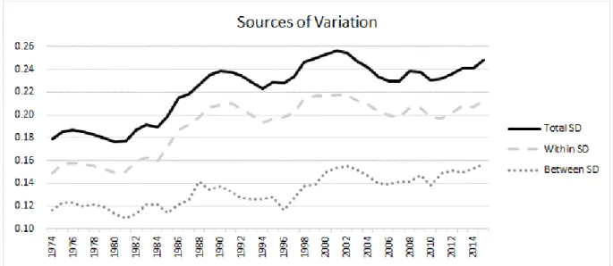
One evident conclusion that can be taken from the analysis of figure 2, is the fact that within-industry variation has been regularly higher than between industry variation. This finding is consistent with the results obtained in table 2 of the previous section. Another

(25)

15

interesting conclusion, is the fact that from 1974 until 2015, within-industry variation was the one that has increased the most, with an increase of 43%. Both total variation and between-industry variation also increased respectively by, 39% and 34%.

Figure 2: Time-series evolution of leverage variation

The three types of leverage variation were calculated for every year, from 1974 until 2015, based only on the book sample. The solid line displays the total variation, which is obtained by doing the standard deviation of all firms’ book leverage ratios for each year. The long-dash line displays within-industry standard deviation defined as √∑ ∑ (𝐿𝑖𝑗−𝐿̅.𝑗)

2 𝑗

𝑖

𝑁−1 . The dotted line represents the between industry variation,

which is obtained by doing the standard deviation of the industry average leverage ratios.

Figure 3: Percentage changes in leverage variation

This figure provides further detail, regarding the percentage changes in the different types of leverage variation, for the period after the 2008 financial crisis.

(26)

16

From the analysis of figure 2, it is possible to conclude that leverage variation increased in the period after the crisis. Nevertheless, figure 3 provides a further understanding regarding the impact of the financial crisis in leverage variation. In 2010 all types of leverage variation decreased, being evident the big drop in the between industry variation that is compensated by a significant increase in the following year. As a note to this analysis, in appendix 5, we are able to observe the evolution of the average book leverage ratios, in the period after the crisis. It is clear that, there was a drop in the firm’s leverage between 2008 and 2010. From 2010 until today, the increase has been steady and persistent, having already surpassed the debt-to-assets ratios before crisis. In general, we are not able to identify a relevant impact of the 2008 financial crisis in the leverage variation variables.

4.3. Importance of industry to firm financial leverage

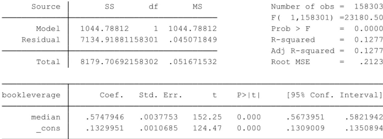
The main objective of this section is to better understand the importance of industry on firms’ leverage ratios. We are able to answer this question by regressing firm-level book leverage ratios on industry year median levels. In our analysis, the industry fixed effects are nested, given that when we are computing the industry median leverage, we exclude the firm from the calculation of the median. For instance, when computing the median for a given firm in a certain four-digit SIC code, we exclude this firm from the calculation of the median. This analysis turns out to be an analysis of variance where the adjusted R-square indicates the importance of industry in explaining the firms’ leverage ratios. The results presented in table 3, demonstrate what Mackay and Philips (2005) and Lemmon et al. (2008) had already concluded: industry explains a small part of the leverage variation. From our regression, we obtain an adjusted R-square of 12.77%, a very similar result to the 13% obtained by Mackay and Philips (2005). It is important to highlight that in our sample we consider all industries, excluding firms form the Finance, Insurance and Real Estate sector from Utilities and from Public Administration, and in Mackay and Philips (2005) they just consider competitive industries (industries with a Herfindahl– Hirschman Index under 1000). It is interesting to notice that the sample used has almost no impact in the importance of industry to the firm financial leverage

(27)

17

Table 3: Importance of industry medians to firm’s leverage ratios

Ordinary least squares regressions of firm’s leverage ratios on industry-year medians for the entire book sample between 1974 and 2015. We estimate the following equation:

𝐿𝑖𝑗𝑡 = 𝛽 ∗ 𝑖𝑛𝑑𝑢𝑠𝑡𝑟𝑦 𝑚𝑒𝑑𝑖𝑎𝑛 𝑙𝑒𝑣𝑒𝑟𝑎𝑔𝑒𝑖𝑗𝑡. When calculating the industry medians the firm into

consideration is excluded.

4.4. Level and consistency in within industry variation

All previous sections try to explain how leverage varies and the importance that industries have on the definition of firms’ leverage ratios. At this point, it is evident that most of the leverage variation occurs in firms of the same industry and that industry fixed effects have little explanatory power. As a consequence of these results, our objective for this section is to better understand the within-industry variation. In this respect, we are going to further explore which industries have the highest leverage dispersion and how consistent is this variation across time.

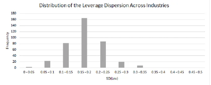
In this section we are going to use our book sample, given that it provides a wider range of data and does not limit our sample to only quoted firms, which could bias our results. To begin our within-industry analysis, we have created a histogram, figure 4, which splits all the 389 four-digit SIC code industries, into 10 variation clusters. The within-industry variation in this case corresponds to the standard deviation of the several within firm means, for each industry. It is important to refer that the standard deviation that represents the leverage dispersion inside an industry must be limited between 0 and 0.5. The reason for this limitation resides in the fact that we have limited book leverage ratios to rely into the closed unit interval, therefore, a minimum of 0 (no dispersion) and a maximum of 0.5 will occur when half of the firms in the industry have no leverage and half only have debt in their capital structures. According to figure 4, 165 industries rely on the interval between 0.15 and 0.2,

_cons .1329951 .0010685 124.47 0.000 .1309009 .1350894 median .5747946 .0037753 152.25 0.000 .5673951 .5821942 bookleverage Coef. Std. Err. t P>|t| [95% Conf. Interval] Total 8179.70692158302 .051671532 Root MSE = .2123 Adj R-squared = 0.1277 Residual 7134.91881158301 .045071849 R-squared = 0.1277 Model 1044.78812 1 1044.78812 Prob > F = 0.0000 F( 1,158301) =23180.50 Source SS df MS Number of obs = 158303

(28)

18

being this, the interval with the maximum number of industries. By observing the histogram we are able to conclude that it follows a symmetric distribution.

Figure 4: Distribution of the leverage dispersion across industries

The histogram presents the number of industries that have a within-industry dispersion inside the clusters presented in the horizontal axis. The within-industry variation is calculated as the standard deviation of the several within firm mean, for each industry and it is constrained between 0 and 0.5. For the construction of this histogram it was used the book sample, which have 389 four-digit SIC code industries.

The terms “level” and “consistency” must be defined, to facilitate the explanation of the following analysis. The term “level” is referred to the amount of leverage dispersion inside some industry and the term “consistency” is mentioned to the variability that this “level” suffers across time. In other words, an industry with a low level but with a high consistency is an industry, in which firms have similar leverage ratios and that this situation is constant over time.

The first step of this analysis is to compute the within-industry variation, which is computed as the standard deviation of the firm’s leverage ratios for the different industries per year, from 1974 until 2015. Next, for each year all the industries are ranked according to the within-industry variation, being attributed the value of 1 to the industry with the lowest standard deviation for that year. The third step in this process is to compute the time series mean and standard deviation of the ranking3_{values for each industry. The time series mean}

provides us information regarding the “level” of within-industry variation, and the standard deviation informs us about the “consistency” of the within-industry variation.

3_{We decided to use the ranking values, because in this analysis we just care about the relative position and}

(29)

19

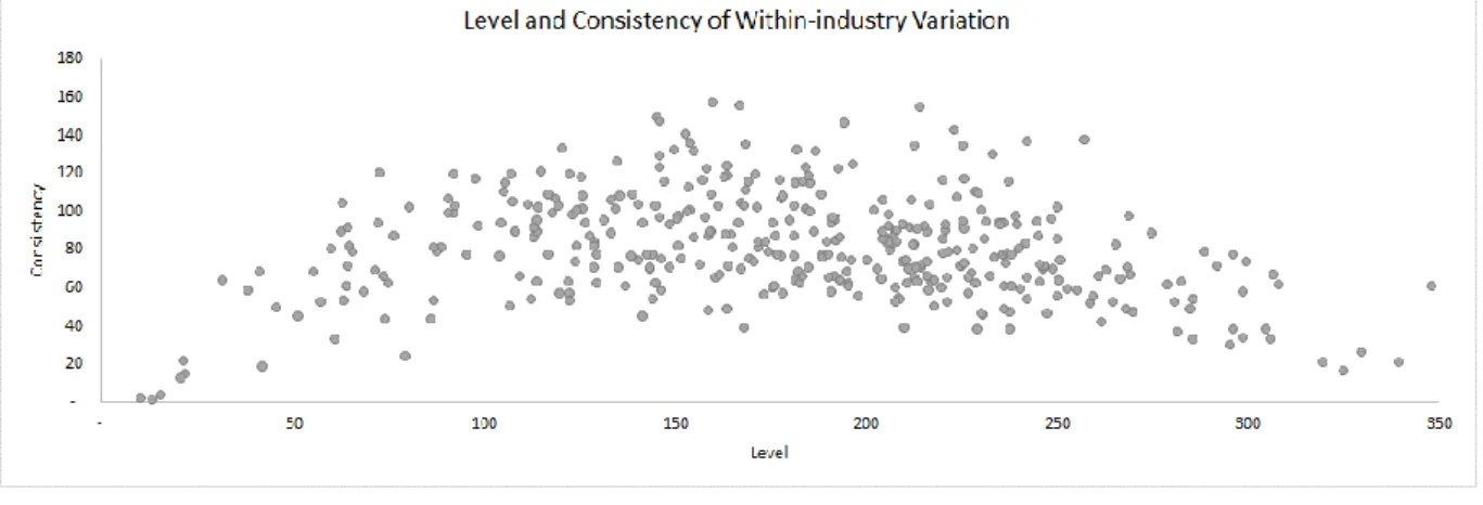
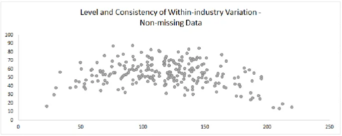
With the purpose of better understanding how “level” and “consistency” are related, we built a scatter plot, presented in figure 5. Each point presented in the image corresponds to a different industry, 389 points in total, which matches the number of industries. The horizontal axis illustrates the variable “level”, so the points that are located to the right have a higher capital structure dispersion. The vertical axis corresponds to the variable “consistency”, so the points that are located on the upper side of the graph have a lower “consistency”. It is important to reaffirm that “consistency” is calculated as the standard deviation of the ranking values for each industry, so the higher the standard deviation the lower the “consistency”.

Figure 5: “Level” and “consistency” of within-industry variation

The data used for the construction of the scatter plot was the book sample. First, it is calculated for each year, the within-industry variation as the standard deviation of the firms’ leverage ratios per industry. Then all the industries are ranked according to the within-industry variation, for each year. Finally, it is calculated the time series mean (“level”) and standard deviation (“consistency”) of the ranking values for each industry.

The previous analysis could be affected by the fact that some industries have no data for some years, which could have an influence in the ranking levels. In order to overcome this problem, we repeated all the previous methodology, but this time, we only included industries that had data for all years between 1974 and 2015. By applying this restriction, our sample ended up with 236 industries. Below we are able to find figure 6, which was built in the same way as figure 5, instead of using the entire sample, it was only considered the 236 industries that had data for the whole data period.

(30)

20

Figure 6: “Level” and “consistency” of within-industry variation, for industries with

non-missing data from 1974 until 2015

This scatter plot was built following the exact same methodology as the one used in figure 5. The only difference relies on the data used, since in this figure, we only consider industries with a value for within-industry variation for all years in the period between 1974 and 2015.

From the analysis of figure 5 and 6, we can conclude that both figures share the same the inverted U shape. This finding allow us to conclude that the industries with the highest level of “consistency” are the ones with the highest and the lowest “level”. In other words, the industries that have the highest or the lowest capital structure dispersion tend to remain this way for long periods of time. This conclusion is very important and introduces to a new stylized fact in this area of research.

In addition to the figures 5 and 6, we are going to provide tables 4 and 5 with the top and bottom 30 four-digit SIC industries in terms of mean (“level”) and standard deviation (“consistency”) of the rankings computed above. It is important to explain again that industries that are part of the top mean correspond to industries with a high capital structure dispersion, and industries at the top standard deviation correspond to industries that see their capital structure dispersion change a lot across the different years. Table 4 includes all the data in book sample, while table 5 only includes industries that had data for all years between 1974 and 2015, in the same way as figure 6 was constructed. Both tables, have some highlighted cells in the columns that correspond to the top and bottom standard deviation. The cells marked by the light grey are the industries that can be found in the mean bottom 30. In contrast, the cells marked by the dark grey are the industries that can be found in the mean top 30. According to table 4, we can observe that 21 out of 30 of the industries presented in the bottom standard deviation (high consistency) are presented in the top/bottom mean. This finding confirms the idea of an inverted U shape in figure 5. Still in table 4, it is possible to

(31)

21

observe that there is no industry in the top standard deviation present in the top or bottom mean.

(32)

22

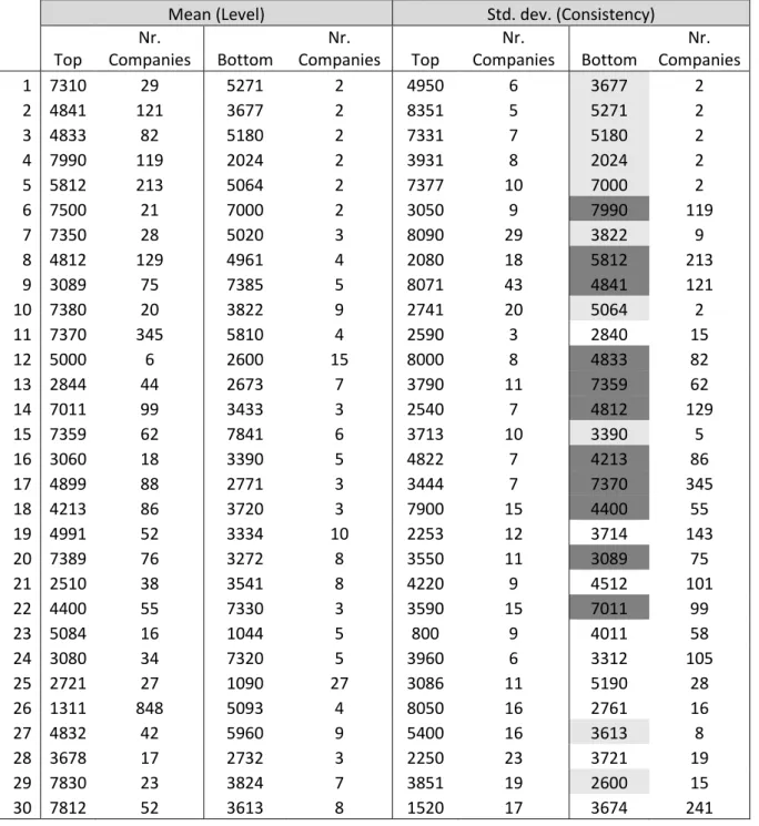
Table 4: Top and bottom 30 industries in terms of “level” and “consistency”

The data used for the construction of this table was the book sample. From the values obtained of the time series mean (“level”) and standard deviation (“consistency”) of the ranking values, we present in this table the top and bottom 30 industries. The cells marked by the light grey are the industries that can be found in the mean bottom 30. In contrast, the cells marked by the dark grey are the industries that can be found in the mean top 30.

Mean (Level) Std. dev. (Consistency)

Top Nr. Companies Bottom Nr. Companies Top Nr. Companies Bottom Nr. Companies 1 7310 29 5271 2 4950 6 3677 2 2 4841 121 3677 2 8351 5 5271 2 3 4833 82 5180 2 7331 7 5180 2 4 7990 119 2024 2 3931 8 2024 2 5 5812 213 5064 2 7377 10 7000 2 6 7500 21 7000 2 3050 9 7990 119 7 7350 28 5020 3 8090 29 3822 9 8 4812 129 4961 4 2080 18 5812 213 9 3089 75 7385 5 8071 43 4841 121 10 7380 20 3822 9 2741 20 5064 2 11 7370 345 5810 4 2590 3 2840 15 12 5000 6 2600 15 8000 8 4833 82 13 2844 44 2673 7 3790 11 7359 62 14 7011 99 3433 3 2540 7 4812 129 15 7359 62 7841 6 3713 10 3390 5 16 3060 18 3390 5 4822 7 4213 86 17 4899 88 2771 3 3444 7 7370 345 18 4213 86 3720 3 7900 15 4400 55 19 4991 52 3334 10 2253 12 3714 143 20 7389 76 3272 8 3550 11 3089 75 21 2510 38 3541 8 4220 9 4512 101 22 4400 55 7330 3 3590 15 7011 99 23 5084 16 1044 5 800 9 4011 58 24 3080 34 7320 5 3960 6 3312 105 25 2721 27 1090 27 3086 11 5190 28 26 1311 848 5093 4 8050 16 2761 16 27 4832 42 5960 9 5400 16 3613 8 28 3678 17 2732 3 2250 23 3721 19 29 7830 23 3824 7 3851 19 2600 15 30 7812 52 3613 8 1520 17 3674 241

(33)

23

After a more careful analysis of table 4, we start to observe a very interesting pattern across the number of firms within each of the different industries presented. The industries that are more consistent in terms of within-industry variation are the ones with a very high or very low number of firms. The bottom five standard deviation is composed of industries that are only composed of 2 firms. The same can be observed from the bottom mean column, in which industries with the lowest capital structure dispersion are mainly composed of less than 5 firms.

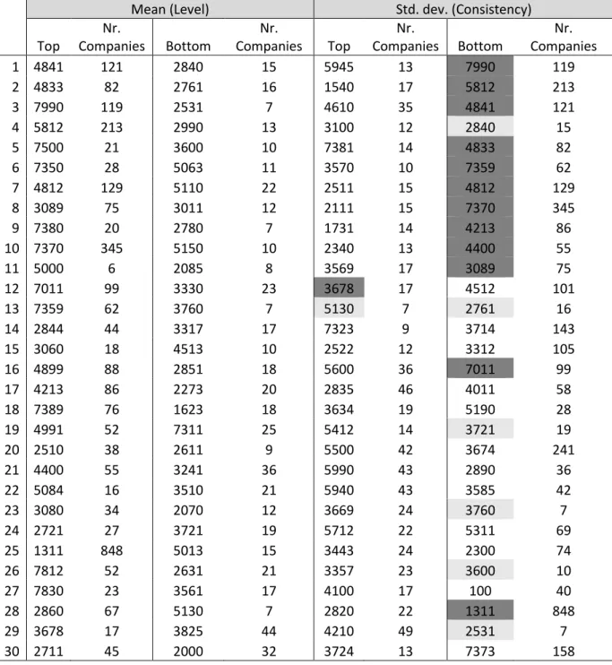
All these problems lead us to create the already mentioned sub-sample formed of only 236 industries. Again this sub-sample was created by only including industries that had data for all years between 1974 and 2015. With this sub-sample was created table 5, in the exact same way as table 4. From table 5, we notice that all the problems of the previous table disappeared. We still notice that the most consistent industries are the ones with a large number of firms. This finding is perfectly justifiable because in an industry with many firms, any change in the capital structure of a firm has a very low impact in the within-industry variation for that industry.

We can also conclude that 18 out of 30 of the industries presented in the bottom standard deviation (high consistency) are presented in the top/bottom mean. If we compare both tables, it is evident the decrease in the number of light grey highlighted cells, given the elimination of industries with a small number of firms. In the bottom standard deviation the light grey cells decreased from 10 to 6 and the dark grey cells increased from 11 to 12.

In table 5, for the first time we have industries with very low consistency presented in the top and bottom mean. Nevertheless, it is interesting to notice that those industries are located at the 29th_{and 28}th_{position, respectively.}

(34)

24

Table 5: Top and bottom 30 industries in terms of “level” and “consistency”, for industries

with non-missing data from 1974 until 2015

This table was built following the exact same methodology as the one used in table 4. The only difference relies on the data used, since in this figure, we only consider industries with a value for within-industry variation for all years in the period between 1974 and 2015. The cells marked by the light grey are the industries that can be found in the mean bottom 30. In contrast, the cells marked by the dark grey are the industries that can be found in the mean top 30.

Mean (Level) Std. dev. (Consistency)

Top Nr. Companies Bottom Nr. Companies Top Nr. Companies Bottom Nr. Companies 1 4841 121 2840 15 5945 13 7990 119 2 4833 82 2761 16 1540 17 5812 213 3 7990 119 2531 7 4610 35 4841 121 4 5812 213 2990 13 3100 12 2840 15 5 7500 21 3600 10 7381 14 4833 82 6 7350 28 5063 11 3570 10 7359 62 7 4812 129 5110 22 2511 15 4812 129 8 3089 75 3011 12 2111 15 7370 345 9 7380 20 2780 7 1731 14 4213 86 10 7370 345 5150 10 2340 13 4400 55 11 5000 6 2085 8 3569 17 3089 75 12 7011 99 3330 23 3678 17 4512 101 13 7359 62 3760 7 5130 7 2761 16 14 2844 44 3317 17 7323 9 3714 143 15 3060 18 4513 10 2522 12 3312 105 16 4899 88 2851 18 5600 36 7011 99 17 4213 86 2273 20 2835 46 4011 58 18 7389 76 1623 18 3634 19 5190 28 19 4991 52 7311 25 5412 14 3721 19 20 2510 38 2611 9 5500 42 3674 241 21 4400 55 3241 36 5990 43 2890 36 22 5084 16 3510 21 5940 43 3585 42 23 3080 34 2070 12 3669 24 3760 7 24 2721 27 3721 19 5712 22 5311 69 25 1311 848 5013 15 3443 24 2300 74 26 7812 52 2631 21 3357 23 3600 10 27 7830 23 3561 17 4100 17 100 40 28 2860 67 5130 7 2820 22 1311 848 29 3678 17 3825 44 4210 49 2531 7 30 2711 45 2000 32 3724 13 7373 158

(35)

25

4.5. Characteristics of industries with high and low capital structure

variation

Now that we already know which industries have the highest and lowest capital structure dispersion, the objective of the following analysis is to understand which industry characteristics differ the most between these two groups of industries. In this section we are going to focus only on the bottom and top mean industries presented in table 5. Taking into consideration the purpose of this section, the industries to be studied are the ones at the top and bottom level, since we are only interested in the industries with the highest and lowest within-industry variation, and not about how consistent is this capital structure dispersion. In appendix 6, it is provided the names of the industries that are going to be further studied in this section.

The variables chosen to characterize the industries at the top and bottom within-industry variation were the ones that according to Almazan and Molina (2002), MacKay and Phillips (2005), Lemmon et al. (2008) and Graham and Leary (2011) were the most relevant in explaining both leverage and capital structure variation. All variables definitions are located in the appendix 2.

The first variable is the time series average of the different within-industry variations. The variable is named as Average yearly SD(Lev). This variable provides an idea of the dimension of the capital structure dispersion in the top and bottom industries. From table 6, we confirm that industries at the top have a higher capital structure variation. The average within-industry variation for the top industries is 0.23, against the 0.11 from the bottom industries.

The second variable to be studied is the number of firms per industry. From table 5, we can understand that industries with the highest capital structure dispersion are the ones with a larger number of firms. If we reflect on this observation, actually it makes sense that industries with a large number of firms tend to have a higher diversity on the way that those firms choose its leverage ratios. According to table 6, we understand that top industries have a significant higher standard deviation in terms of the number of firms (154.66 vs 8.73), something that we can also observe by the difference between the maximum and minimum values. One interesting observation is the fact that the top median (53.50)4_{is higher than the}

maximum number of firms (44) in the bottom industries. From table 7, we observe a positive

4_{In excel if there is an even number of numbers in the set, then median calculates the average of the two}

(36)

26

correlation (0.30), which confirms our initial idea that capital structure dispersion increases with the number of firms.

The third variable was inspired in the study MacKay and Phillips (2005), which defends that firms near the industry median capital–labor ratio use less financial leverage than firms that deviate from the industry median capital–labor ratio. Based on this observation we can conclude that the higher the capital-labor dispersion the higher the capital structure dispersion. In our study we decided to use the coefficient of variation, as proxy for the technology (capital-labor) dispersion inside each industry. By comparing the means for the top and bottom industries, it is clear that there is a higher technology variation in the industries with the highest capital structure dispersion. It is also possible to observe that the median in the most dispersed industries is higher than the maximum of the bottom industries. From table 7, we observe a positive correlation (0.41), which confirms our initial idea that capital structure dispersion increases with the technology dispersion. These results are consistent with the results from MacKay and Phillips (2005).

The fourth variable is the proportion of capitalized lease obligations of the total book assets. According to Almazan and Molina (2002), intra-industry capital structure dispersion is greater in industries in which firms use leasing more intensively. From the results obtained in table 6, the difference between the top (1.5%) and bottom mean (1.1%) is not very significant. This variable is very problematic given the possibility that firms have to opt between operating and capital leases. In the end the impact of this choice on the firm’s capital structure is very high. Taking this into consideration, it could happen that industries that use more leasing have a higher capital structure dispersion, motivated in a large part to accounting choices. From table 7, we observe a small positive correlation (0.18), which confirms our initial idea that capital structure dispersion increases little in industries that use leasing more intensively.

The fifth variable was inspired in the study of Titman and Wessels (1988), which suggests the ratio between selling expenses over sales, as a proxy to the product uniqueness. According to Almazan and Molina (2002) the higher the product uniqueness inside an industry, the more specific is the firm in terms of leverage ratio and other firm’s financials, leading to a higher intra-industry leverage variation. From the analysis of table 6, we confirm that top industries have a higher product uniqueness on average when compared to the bottom industries. Also note that the value for the median is a higher for industries at the top within industry variation. An alternative proxy to measure product uniqueness is the ratio between research and development over the value of sales. In consonance to the previous proxy, we notice that

(37)

27

industries at the top within-industry variation are more R&D intensive. From table 7, we observe that both proxies for product uniqueness present a small positive correlation (0.17), which confirms our initial idea that capital structure dispersion increases little with the level of product uniqueness.

The next variable to be analyzed is firm age, which we proxy by counting the number of firm-year observations for each company. It is possible to conclude that industries with low capital structure dispersion tend to have a higher longevity. From table 7, we observe one of the most significant correlations (-0.57), which confirms that capital structure dispersion decreases with the firm’s longevity.

The eighth variable to be analyzed is the Herfindahl–Hirschman Index (HHI). This variable measures the market concentration, through the market share of the several firms within each industry. The higher the HHI the more concentrated is the industry, that is, the level of competition is smaller. In the other hand, the smaller the HHI the more competitive is the industry, in other words, the level of competition is higher. According to table 6, it is evident that industries with a higher capital structure dispersion tend to be more competitive. The average HHI for the top industries is 2822, in contrast to the bottom industries that is 4314. The relation between the level of competition and the intra-industry leverage dispersion was not consensual in the literature. According to MacKay and Phillips (2005), the leverage in competitive industries is reduced and more dispersed. In contrast, Almazan and Molina (2002) defends that intra-industry capital structure dispersion is greater in industries that are highly concentrated. From table 7, we observe a negative correlation (-0.41), which confirms that capital structure dispersion increases with the level of competition. Our results corroborate with the results provided by MacKay and Phillips (2005).

The variable asset tangibility was inspired by Lemmon et al. (2008), who report that asset tangibility captures most of the variance decomposition. Asset tangibility is the ratio of net property, plant and equipment over total assets. From the analysis of table 6, we conclude that top industries have slightly more tangible assets than the bottom industries. By analyzing table 7, we observe a positive correlation (0.22), which confirms our initial idea that capital structure dispersion increases with the assets tangibility.

The tenth variable to be analyzed is the Z-score, which is used to predict the probability that a firm will go into bankruptcy. The higher the value for the Z-score the better is the financial health of the firm. It is evident that industries at the top intra-industry dispersion, have a worse financial situation than firms in the bottom dispersion. From table 7, we observe a significant negative correlation (-0.50), which confirms that capital structure dispersion is

(38)

28

associated to higher probability of default. These results could be associated to the previous observation that firms in the top dispersion tend to have a shorter longevity.

The next variable represents the firm size, which is equal to the total book assets. Table 6, show us that on average industries with low capital structure variation are larger than the industries with a high variation. From table 7, we observe a small negative correlation (-0.15), which endorses the previous conclusion that capital structure dispersion decreases with the size of firms.

In terms of profitability and risk, the differences between the two groups of industries are not very significant, but we can say that the industries at the top within-industry variation are slightly more profitable and more risky. The results presented at table 7, confirm a small positive relation between the intra-industry dispersion and the level of risk and profitability.

The fourteenth variable to be analyzed was developed by us, with the purpose of understanding if capital structure dispersion is related to the fact that companies pay dividends. For all firm-year observations, if a company paid dividends, then it will receive the value of 1, in any other circumstance it would receive the value of 0. The next step is to compute for each firm the time series mean, and finally the cross section average across firms within the same industry. For our analysis, the higher the value of our variable “dividend payer” the higher the number of firms in that industry paying dividends. Table 6 shows that industries at the bottom intra-industry variation tend to have more firms paying dividends. In the same line of reasoning, table 7 present a significant negative correlation (-0.44), which confirms that capital structure dispersion is associated with a smaller number of firms paying dividends.

Finally, we observe that the top industries are more leveraged than the bottom ones, as illustrated by the difference in the average leverage ratio of high dispersed industries (39%) to low dispersed industries (26%). From table 7, we observe the most significant correlation (0.67), which confirms our initial idea that capital structure dispersion is linked to more indebted firms.

(39)

29

Table 6: Characteristics of top and bottom intra-industry dispersion industries

The most significant variables in the literature explaining both leverage ratios and capital structure dispersion were selected, in order to trace a profile of the type of industries with the highest and lowest capital structure dispersion. The industries selected were the ones at the top and bottom level in table 5. The construction of the following variables is provided in appendix 2.

Top within industry variation Bottom within industry variation

Mean Median Std..Dev. Min. Max. Mean Median Std..Dev. Min. Max.

Average yearly SD(Lev) 0.23 0.23 0.02 0.21 0.28 0.11 0.11 0.02 0.08 0.13

Nr. companies per industry 96.87 53.50 154.66 6.00 848.00 16.73 15.50 8.73 7.00 44.00

CV(capital / labor) 2.09 1.59 1.88 0.56 10.18 0.75 0.76 0.24 0.31 1.49

Lease / assets 0.02 0.01 0.02 0.00 0.05 0.01 0.01 0.01 0.00 0.03

Sell exp / sales 0.77 0.22 1.60 0.02 8.55 0.31 0.18 0.63 0.06 3.63

Firm age 11.97 11.70 2.58 7.40 17.67 16.64 16.13 4.07 9.62 25.80 HHI 2822.41 2119.63 1723.67 883.27 8863.52 4314.48 4085.11 1670.49 2242.35 7883.91 R&D / Sales 0.11 0.00 0.31 0.00 1.27 0.05 0.00 0.15 0.00 0.76 Tangibility 0.39 0.38 0.18 0.12 0.77 0.30 0.28 0.15 0.10 0.63 Z-score 0.98 0.83 0.92 -0.67 3.08 1.98 2.09 0.84 -0.74 3.59 Firm size 1843.13 1076.27 2594.10 132.57 11158.06 2893.40 1758.63 3891.06 58.63 20255.35 Profitability 0.12 0.13 0.05 -0.02 0.24 0.12 0.12 0.04 -0.02 0.20 Risk 0.06 0.05 0.03 0.03 0.13 0.06 0.05 0.02 0.03 0.10 Dividend payer 0.45 0.44 0.12 0.17 0.70 0.59 0.56 0.18 0.22 0.90 Book leverage 0.39 0.38 0.09 0.16 0.57 0.26 0.26 0.06 0.15 0.39