Female Labor Supply and Public Spending
Tiago V. de V. Cavalcanti† Jos´e Tavares‡
July 2003
Abstract
The increase in income per capita is accompanied, in virtually all countries, by two changes in the structure of the economy: an increase in the share of government spending in GDP and an increase in female labor force participation. This paper suggests that the changes in female labor force participation and government size are not just coincident in time, they are causally related. We develop a growth model with endogenous fertility, labor force participation and government size to illustrate this causal link. When gov-ernment consumption and/or subsidies decrease the cost of performing household chores - including, but not limited to child rearing and child care - an increase in the female market wage leads to an increase in labor force participation by women and a demand for higher government spending. As women make the decision to work outside the home, they increase their demand for services typically provided by the government, such as education and health care, which, in turn, decrease the cost of home and family activi-ties that are overwhelmingly performed by women. We show, for a wide cross-section of developed and developing countries, that higher female participation rates in the labor market are positively associated with larger governments. We investigate the causal link by instrumenting for female labor force participation with the prevalence of contraceptive methods and the relative price of household appliances. Female labor force participation is found to cause an increase in government size, with a 10 percent rise in the former leading to a 6.5 to 9 percent rise in the latter. This effect is stronger for government consumption than for government subsidies and is robust to the country sample, time period, and a set of controls in the spirit of Rodrik (1998).
JEL Classification Numbers: O1, J1, E62
Keywords: Economic Development, Female Labor Supply, Government Size, Home Ac-tivities.
∗This paper has benefitted from the financial support of ´Egide and Nova Forum at Universidade Nova. We are indebted to Jeremy Greenwood, Jos´e Ferreira Machado, and Guillaume Vandenbroucke for helpful suggestions and comments. We thank Daniel Santos and Paulo David for access to some of the data used in the paper.
†Faculdade de Economia, Universidade Nova de Lisboa, Portugal. Email: cavalcan@fe.unl.pt.
‡Corresponding Author: Jos´e Tavares, Faculdade de Economia, Campus de Campolide, Universidade Nova de Lisboa, Portugal 1099-032. Tel.: +351-21-380-1669; fax: +351-21-388-6078; email: jtavares@fe.unl.pt.
1
Introduction
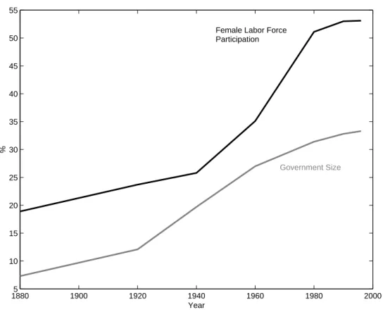
In virtually all developed and developing economies, the growth of per capita income has been accompanied by two major structural changes in the economy: the share of government spending in Gross Domestic Product (GDP) has increased apace with a rise in the participa-tion of women in the labor force. The share of total government spending in GDP increased 10 percent in OECD in the last twenty years,1 the continuation of a long trend in growth of government in the twentieth century. Tanzi and Schuknecht (2000) report, for a sample of industrialized countries, an increase in general government spending from 13 percent of GDP in 1913 to 46 percent in 1996. Simultaneously, female labor force participation in the OECD has risen from 28 to 41 percent, while male labor force participation remained constant at 57 percent.2 Goldin (1995) reports that female labor force participation in the United States increased from 3.1 to around 50 percent of the labor force between 1900 and 1980. Figure 1 shows the evolution of female labor force participation and the share of government expen-ditures in GDP in the United States over the last Century.3 This paper suggests that the changes in female labor force participation and government size are not just coincident in time, they are causally related. As women make the decision to work outside the home, they increase their demand for services typically provided by the government, such as education and health care, which, in turn, decrease the cost of home and family activities that are overwhelmingly performed by women. The resulting lower burden of home activities makes it easier for female labor force participation to increase.4
There is a long tradition in economics that attempts to explain the causes of the increase in the size of government. One strand in this literature relates the size of government with the income of the median voter and the expansion of the voting franchise, in the tradition of Tocqueville (1835). In such a vein, Meltzer and Richards (1981) developed a seminal model that links increases in public redistribution to the inclusion of voters from the lower end of the income spectrum. The study by Husted and Kenny (1997) of US states between 1950 and 1988 analyzes the impact of abandoning poll taxes and literacy tests as requirements to vote and finds that the resulting expansion of the franchise led to a rise in redistributive expenditures. The supply of government services, as opposed to pure redistribution, does not seem to respond in the same way to the extended franchise.5 In fact, whether the demand for government services increases as low income voters join the franchise depends on the relative force of an income and a substitution effects: lower income voters tend to use public services
1According to World Bank (2001). 2Also World Bank (2001).
3Blau (1998) shows that participation rates of men actually decreased about 6 percent between 1970 and 1995 and the difference between the participation rates of educated versus less educated men is substantially smaller than that of women’s. See Goldin (1990) for a historical overview of female participation in the labor market in the United States. Olivetti (2001) sums this phenomenon as: “In the past, married women of childbearing age tended to specialize in childrearing and home production activities at the expense of engaging in market work. Now, they do not curb the hours worked in the market.”
4Blau (1998) reports that, in the decade from 1978 to 1988, the number of women work hours at home and in the market reversed from 27/20 to 21/26.
5This is consistent with the results in Peltzman (1980), who finds little relation between the franchise and total government spending in Great Britain, Canada and the United States.
18805 1900 1920 1940 1960 1980 2000 10 15 20 25 30 35 40 45 50 55 Year %
Female Labor Force Participation
Government Size
Figure 1:Female labor force participation and government size in the United States, 1880- 1996. Data for female labor force participation are from Goldin (1990, Table 2.1) and World Bank (2001). Data for the share of government expenditures in GDP are from Tanzi and Schuknecht (2000).
instead of available private substitutes but, on the other hand, demand less public services as a direct consequence of their lower individual income. As Husted and Kenny (1997) points out, the income effect may more than overcome the substitution effect, which is entirely consistent with Wagner’s law suggesting that a rise in a country’s per capita income leads to an increase in the share of public spending in GDP. As in Wagner (1893).
Public spending - redistribution or consumption services - can be valued also as protection against income or employment shocks. In this view, the government provides a safety net, in the form of subsidies, services or public employment. Rodrik (1998) argues for such a rationale for the increase in government services, and finds that government spending is positively related to a greater exposure to external shocks. In the end, a complete explanation of the dramatic growth in government in the twentieth century continues to elude economists. A conspicuous issue is the fact that public spending did not always grow. Public spending started to increase in the early 20th century as income tax systems started to be set up but only after World War I and the massive mobilization of women into the labor force that accompanied it, did the size of government not revert to pre-war levels, as had always
happened.6 Giving women the right to vote was, according to Lott and Kenny (1997), the decisive change that led to a surge in government spending. These authors examine the changes in government spending over time in US states that extended the right to vote to their female population and find that turnout rates rose hand in hand with government spending.
Another issue is how the participation of women in the labor market is affected by public spending. A substantial fraction of the tasks related to home and family that traditionally fell on the shoulders of women,7 such as caring for children, the sick and the elderly, i.e., “redistribution” and insurance roles, have been progressively taken up by the state.8 Public programs that perform such tasks tend to decrease the time women devote to tasks -conspicuously child care and education - allowing increased female labor force participation. Chevalier and Viitanen (2002), for instance, find that the availability of child care increases female labor force participation, suggesting that female labor supply is constrained by the lack of child care facilities.9 Anderson and Levine (1999) find that the responsiveness of female labor market participation to the cost of child care is of the same order of magni-tude of the response to female wages.10 The decision to work outside the home is likely to lead women to demand wider and better provision of the public services that alleviate their unequal burden at home.11 In addition, the risk-reduction motive to increase government spending, the basis for Rodrik (1998) may affect most closely women and the female labor force.12
In this paper we present a growth model with endogenous choice of fertility, female labor force participation and government size. We build on the model of Galor and Weil (1996)
6Lott and Kenny (1997).
7Blau (1998) points out that in the case of married women not in the labor force or men - either single, married, with or without employed wife - there was practically no change in hours worked at home: while married women not in the labor force worked between 33 and 37 hours a week, men worked between 5 and 8 hours.
8Case and Paxson (2000) find that it is children’s mothers that make most investments in children health, namely as regards time consumed in doctors visits and the like. Similarly, Costa and Kahn (2001) argue that the rise in female labor force participation is associated with the reduction in the production of “social capital” at home. Social capital is related to activities that involve spending time with friends and relatives, which have been shown to have a positive impact on the social development of children.
9Surveys of working mothers in the United Kingdom and the United States found that, respectively 20 and 30 percent stated that childcare obligations restricted their labor force participation. Another study found that regional variation in female labor force participation were related to availability of childcare facilities. See Chevalier and Viitanen (2002).
10
In a simulation exercise, they find that a 50 percent decrease in hourly cost of childcare leads to a larger increase in labor force participation than an equal dollar increase in salary for all female groups - independently of child age, marriage status, etc., suggesting the importance of provision of government services to labor force participation.
11Lott and Kenny (1997) mention the consistent differences between the voting patterns of men and women. Women are more likely to be liberal and vote for the Democrat presidential candidate traditionally associated with the defense of a larger role for the government.
12Government jobs in teaching and health tend to be filled primarily by women, as documented in Rosen (1996) for Sweden. Lott and Kenny (1997) mention that 55 percent of white-collar government jobs in the US are filled by women. Goldin (1995) shows that the percent of women in the total clerical jobs workforce increased from 15 to 62 percent of the total between 1900 and 1950.
of fertility and growth by introducing a government sector whose size is endogenous. We assume that higher public spending - either in subsidies or in public services - decreases the cost of raising children by substituting for women’s time with household chores. In our model, the rise in income increases the opportunity cost of not working and leads women to progressively join the labor force by increasing their hours of work.13 As female labor force participation increases, there is a reduction in the total cost of raising children for two reasons: the total time at home (and number of children reared) decreases and the time cost per child falls as the increase in public spending partly substitutes for home “production” of care, education, etc.14 One of the possible paths for the economy is for the income rises to be accompanied by higher female labor force participation, and higher government spending. Unlike previous studies that concentrate on the extent of the franchise, we examine female labor force participation, which allows us to directly test our hypothesis using a wide panel data set of developed and developing economies in the last four decades.15 We test the relationship between female labor force participation and government size and find that higher female labor force participation is significantly and positively related to government spending as a share of GDP - in the form of government consumption, subsidies and transfers and total spending. The result is robust to the inclusion of time and country fixed-effects and the inclusion and the expansion of the set of control variables in Rodrik (1998). Furthermore, the inclusion of male as well as female labor force participation shows that the former does not display the same association with government spending, rather the contrary. An increase in female labor force participation of 10 percent leads to an increase in government spending of about 2,5 percent as a share of GDP.16 We are able to assess causality by instrumenting for female labor force participation. In the spirit of Greenwood and Seshadri (2003) and Greenwood et al (2002a, 2002b), who find a relationship between technological progress in productive home capital - such as appliances - labor force participation and fertility, we have compiled an index of the relative price of home appliances, which we use to instrument for the effect of female labor supply on government size.17 For a wider sample, we use the
13Goldin (1995) shows that female labor force participation of married women tends to decrease and then increase as national income rises. This decline is due to a strong initial income effect that is later dominated by a substitution effect. Goldin (1995) suggests that when women have poor human capital and their wage in the market is only connected with manual work, social stigma adds further resistance to female participation; as women become educated, this stigma disappears. Goldin (1995) shows that high-school graduation rates were higher for women during the whole period from 1910. Blau (1998) shows that the more educated the woman, the more it tends to participate in the labor market, with those with more than 16 years of education with a 83 participation rate compared with 47 for those with less than 12 years. Acemoglu, Autor and Lyle (2002) find that, after the increase in female labor force participation in the wake of World War II, women were closer substitutes for male high-school graduates than to less than high-school or the lowest skill males.
14
It is important to make clear that childrearing is used as a metaphor for any time-consuming task at home that tend to be performed mostly by women.
15Iversen and Soskice (2001) find, for a small sample of European countries, that female labor force par-ticipation has a positive correlation of 0.51 with the amount of redistribution, measured as the difference between pre and post-tax income.
16This effect is quantitatively of the same order of magnitude as the effect of trade on government spending uncovered in Rodrik (1998).
17As stated in Greenwood, Seshadri and Yorukoglu (2002b) “It seems unlikely that the small rise in the relative income of a female worker could explain the dramatic rise in labor force participation. It is more likely that the rise in overall real wages, in conjunction with the introduction of labor-saving household appliances,
prevalence of contraception as the instrumental variables. In both cases we confirm our main result, uncovering a positive, significant and robust effect of female labor supply on public expenditures.
The paper is organized as follows. Section 2 presents the model and a numerical example that illustrates the relationship between female labor supply and government size. Section 3 presents an empirical test of the relationship, checks for robustness and investigates causality. Section 4 concludes.
2
The Model
Our model adds an endogenously determined government sector into a growth model with labor specialization as in Galor and Weil (1996). The economy is made up of men and women organized as couples. Agents live for three periods. In the first period, as children, women and men are indistinguishable: children do not make any decision, they only consume a fraction of their parents’ time endowment, in the form of parental care and general childrearing. In their second period of life agents become adults and men and women differ as to their labor endowment: men are endowed with one unit of physical labor and one unit of mental labor while women are endowed with mental labor.18 In this second period, couples make their fertility choices and allocate their time between working and raising children. In the third period, each couple consumes the life savings.
Technology
The production technology uses capital, Kt, mental labor, Lmt , and physical labor, L p t, to produce output, Yt, according to a constant returns to scale production function. More specifically,
Yt= A[αKtρ+ (1 − α)(Lmt )ρ]
1
ρ + BLp
t, (1)
where A > 0, B > 0, α ∈ (0, 1), and ρ ∈ (−∞, 1). Given the technology and the input prices, the representative firm chooses inputs so that profits are maximized.19 It is convenient, however, to rewrite the variables in per-couple term. Since the number of couples in the economy is the same as the number of total physical labor input, define: yt = LYtp
t, kt=
Kt
Lpt, explains the rise in female labor-force participation.” In our paper government size is the missing variable that explains the surge and participation and the relative price of appliances is used as instrumental variable in the empirical test of this hypothesis.
18As will become clear, this assumption makes our model deliver two facts that are borne by the available evidence: the existence of a gender wage gap and its decrease over time as income per capita increases. Blau (1998) reports that weekly wage ratios of women increased about 31 percent between 1970 and 1994 while men’s weekly wage rates increased only by 3 percent, decreasing the male/female wage ratio. The increase in women’s wages was concentrated on the wages of educated women (despite a relatively higher increase in supply) and was related to occupation, experience and education.
mt= L
m t
Lpt as output per couple, capital per couple and the ratio of mental to physical labor.
The first order conditions associated with the representative firm’s problem are:
wpt = B, (2) wmt = A(1 − α)[αktρ+ (1 − α)(mt)ρ] 1−ρ ρ mρ−1 t , (3) rt = Aα[αktρ+ (1 − α)(mt)ρ] 1−ρ ρ kρ−1 t , (4)
so that the wage rate of physical labor is exogenous and constant, and the wage rate of mental labor and the interest rate depend on capital per couple and the ratio of mental to physical labor.
Preferences
Couples draw utility both from consumption in the third period of life and the number of children. Let nt be the number of children born at period t, and ct+1 be the consumption of a couple in their third period of life. Preferences are represented by20
Ut= γ ln nt+ (1 − γ) ln ct+1, γ∈ (0, 1). (5) where γ represents the relative weight of children in the couple’s utility function.
Government
Consider now that there is a government sector in this economy. The government raises public revenues through a proportional tax, τtand spends it as gt, the per-couple government spending so that budget is balanced throughout. Public spending is assumed to decrease the per-child cost of raising children. In the spirit of Greenwood, Seshadri and Vandenbroucke (2002a), we assume that children are costly and the “production function” associated with raising children is
nt= φ[ht(1 + gt)]β, φ >0, β ∈ (0, 1], (6) where htis the time that parents devote to raising children. Solving (6) for htgives the time cost of nt children ht= ( nt φ) 1 β 1 1 + gt . (7)
We can also interpret htas the time couples spend at home, and 2 − htthe time devoted to market activities.
20Given the functional form of the utility function, it is clear that the introduction of consumption in the second period of life does not change any of the results.
Budget Constraint
Notice that the opportunity cost of raising children is higher for a man, (1−τt)(wpt+wmt ), than for a woman, (1 − τt)wtm. Therefore, if ht ≤ 1, only the wife spends time raising children.21 In the case where h
t > 1 both will raise children but only the husband will work.22 The couple’s budget constraints are:
st ≤ (1 − τt)(wtp+ wtm+ (1 − ht)wtm), if ht≤ 1, (8) st ≤ (1 − τt)(wtp+ w m t − (ht− 1)(wmt + w p t)), if ht≥ 1. (9) where st represents savings and the right-hand side shows net income of the couple.
In the last period of life, consumption by the couple must satisfy
ct+1 = (1 + rt+1)st. (10)
Couples choose the number of children, nt, and savings, st, to maximize (5) subject to (7)- (10). The fertility decision satisfies23
ht= ( nt φ) 1 β 1 1 + gt = γβ (1 − γ) + γβ[2 + wtp wm t ], if ht≤ 1, (11) ht= ( nt φ) 1 β 1 1 + gt = 2γβ (1 − γ) + γβ, if ht>1. (12) In order to guarantee that women will eventually participate in the labor market for any tax rate, we must assume that (1−γ)+γβ2γβ ≤ 1. This implies that γ ≤ 1+β1 , so that couples have to assign a minimum weight on consumption for it to be worthwhile to increase labor market participation. Thus,
ht= ( nt φ) 1 β 1 1 + gt = min{1, γβ (1 − γ) + γβ[2 + wtp wm t ]}. (13)
21In this model, as in Galor and Weil (1996), the specialization of male and female into market and home activities is a consequence of assuming one unit of male labor produces one unit of physical labor and one unit of mental labor while one unit of female’s labor produces only mental labor.
22This is consistent with the empirical fact that male labor force participation rates tend to be higher than their female equivalent.
23The fact that fertility affects labor market participation has been documented in Jacobsen, Pearce III and Rosenbloon (1999). These authors use the unexpectedness of twin births as an exogenous variation in fertility to determine the causal effect of fertility on married women’s labor supply and earnings. They find that the impact is appreciable and has increased from 1980 to 1990.
The wage of physical labor is constant, since wpt = B, while the wage of mental labor increases with capital accumulation. Therefore, female labor force participation increases as the relative wage of mental labor increases (decreasing the gender wage gap), which increases the opportunity cost of staying at home. Private savings are given by
st = (1 − γ) (1 − γ) + γβ(1 − τt)(2w m t + w p t) if ht≤ 1, (14) st = (1 − τt)(wtm+ w p t) if ht= 1. (15)
Tax Rate Determination
The public sector maintains a balanced budget at every point in time. Therefore,
gt= τt(wpt + wtm) + τt(1 − ht)wmt . (16) Using (13) into (16) yields
gt= ( τt(1−γ)+γβ(1−γ) (2wmt + w p t) if ht<1, τt(wmt + w p t) if ht= 1. (17)
We assume that τt is endogenously determined in each period by a vote of the adult population. Since we assumed a homogenous population and given logarithmic utility there is no conflict of interest. Given the list of factor prices wt= (wtm, w
p
t, rt+1) and the tax rate, the indirect utility of the representative couple is
V(wt; τt) = γln{[ht(wt; τt)(1 + g(wt; τt))]βφ} + (1 − γ) ln[(1 + rt+1)st(wt; τt)] if ht(wt; τt) < 1, γln[(1 + g(wt; τt))βφ] + (1 − γ) ln[(1 + rt+1)s(wt; τt)] if ht(wt; τt) = 1. (18)
The representative couple chooses the tax rate τtto maximize the indirect utility function, i.e.,
τt∗ = arg max τt≥0
V(wt; τt), (19)
subject to (17) and (13). There are two effects of an increase in the tax rate. The first is a direct effect, since a higher tax rate decreases net labor income. There is also an indirect effect: a higher tax rate increases government revenues and public spending makes it easier
to devote hours to market activities while increasing the effective time available to both home and market activities. This tradeoff will result in a chosen tax rate, which is given by:
τt∗ = ( γβ (1−γ)+γβ− (1−γ) ((1−γ)+γβ)(wm t +w p t), if ht(wt; τt) = 1, γβ (1−γ)+γβ−2wm1 t +w p t , if ht(wt; τt) < 1. (20)
Notice that if (20) is negative, then the optimal tax rate is zero. This implies that τt∗ ∈ [0,(1−γ)+γβγβ ). It easy to verify that the tax rate increases with the mental wage. Since the time that couples spend at home htis non-increasing with wtm, this implies that the tax rate increases as couples devote more time to market activities (see (13)).24
Equilibrium
In equilibrium, demand must equal to supply in all markets. In the market for mental labor this means that Lm
t = L p
t(2 − ht), or mt = 2 − ht. Then, using the input market equilibrium conditions, (2) and (3) into (13), yields
ht= min{1, γβ (1 − γ) + γβ[2 + B A(1 − α)[αkρt + (1 − α)(2 − ht)ρ] 1−ρ ρ (2 − h t)ρ−1 ]}. (21)
Using the implicit function theorem it can be shown that (21) defines a function ψ(kt) such that
ht= min{1, ψ(kt)}, with ψ0(kt) < 0 ∀kt≥ 0. (22) (22) determines a critical value k∗ such that
ht= ½
1 for kt≤ k∗,
ψ(kt) for kt≥ k∗, (23)
and ψ(kt) ∈ (0, 1] ∀ kt ≥ k∗. As a consequence, time devoted to home activities decreases with capital accumulation. The condition which equilibrates the capital market is
Kt+1 = Lptst. (24)
24In other words, as female participation in the labor market increases (and male participation remains constant), the preferred tax rate increases.
When the optimal tax rate is positive,25we have that kt+1 = st nt = ( D(wm t + B)1−β for kt≤ k∗, D( wtm 2wm t +B) β (γβ+(1−γ)(1+2wmt +B))1−β ((1−γ)+γβ)1−2β for kt≥ k∗, (25) where D = φ(γβ)β((1−γ)+γβ)(1−γ) 1−β, and wmt = ( A(1 − α)[αktρ+ (1 − α)]1−ρρ , for k t≤ k∗, A(1 − α)[αkρt + (1 − α)(1 − ψ(kt))ρ] 1−ρ ρ (1 − ψ(k t))ρ−1, for kt≥ k∗. (26)
Using (26) into (25) defines a non-linear difference equation kt+1 = ξ(kt). As in Galor and Weil (1996), it is clear that ξ(·) is continuous, and it can be shown that ξ0(k
t) > 0 ∀ kt≥ 0. Moreover, ξ(0) > 0, limkt→0ξ 0(k t) = ∞, and limkt→∞ξ 0(k t) = 0. Therefore, a steady-state equilibrium, ξ(k) = k, exists. However, here as in Galor and Weil (1996), one cannot guarantee that the steady-state equilibrium is unique. In order to see this, notice that if the degree of complementary between capital and mental labor is sufficiently small, then the ξ(·) function is strictly concave for kt∈ (0, kt∗). Specifically, if ρ ∈ [0, 1), then ξ00(kt) < 0 for kt ∈ (0, k∗t). Otherwise, ξ(·) is strictly convex for kt ∈ (0, kt∗). In contrast, for kt∈ (kt∗,∞) we cannot define whether the function ξ(·) is concave or not. Regardless of whether multiple steady states exist, the model generates the following result.
Proposition 1 As the economy develops, then
i. the women’s fraction of time at home activities decreases; ii. per-couple government spending increases; and
iii. the share of government expenditure in total output increases.
Proof. Item (i) follows directly from (23). (ii) follows from (17) and (20). In order to see this, notice that
gt= ( γβ(1−γ) ((1−γ)+γβ)2(wtm+ B) − (1−γ) 2 ((1−γ)+γβ)2, for kt≤ k∗, γβ(1−γ) ((1−γ)+γβ)2(2wmt + B) − ((1−γ)+γβ)(1−γ) , for kt≥ k∗,
which is increasing in capital accumulation. Dividing gtby yt results in item (iii).
Per-couple government spending increases both because income and the tax rate increase as the economy develops. The model, however, might display equilibria where both female labor force participation and fertility increase as the economy develops. The reason is sim-ple. For parents, the only cost of a child is the opportunity cost of being at home. This
opportunity cost is a decreasing function of per-couple government spending and goes to zero as spending goes to infinity. Then, even when female labor force participation is increasing (i.e., ht= (nφt)
1 β 1
1+gt is decreasing), fertility nt might increase, as long as the rate of change
in fertility is lower than that of 1 + gt.26 In addition, the model abstracts from child quality. Considering quality would add force to the transition from high to low fertility proposed in Galor and Weil (2000) and would generate an equilibrium with decreasing fertility, increasing female labor force participation and increasing per-couple government spending.27
The point that we emphasize, however, is the link between female labor force participa-tion and per-couple government spending. Proposiparticipa-tion 1 suggests that the model generates a simple and powerful result: as the relative wages of mental labor increases, couples de-mand higher government spending in activities that facilitate child-rearing, further easing the transition of women into the labor force.
3
Empirical Results
The theoretical model in Section 2 suggests that there is a positive association between the participation of women in the labor force and the size of government. In this section we conduct an empirical test of that relationship, concentrating on the causal direction from labor force participation to government size. This is the novel element in our model, as yet untested in the literature. We use annual data for the years 1960 to 1999 for a wide cross section of developed and developing countries, available from World Bank (2001). Our variable of interest to be explained is the share of total government expenditures in Gross Domestic Product (GDP), as well as its decomposition into Public Consumption and Public Subsidies plus Transfers. As discussed above, if subsidies and/or public consumption decrease the burden of household chores, their share in GDP may increase in response to the desires of working women.28 Our prediction is that, as female labor force participation increases, so will public spending. Our coefficient of interest is associated with the level of female labor force participation in a wider specification explaining government size. The equation we estimate is:
GOV SIZEt= α + β0.F EM ALELF Pt+ β1.Zit+ εt, (27)
26This, of course, depends on the functional form of the home production function n
t= φ[ht(1 + gt)]β. If we have assumed that nt= φ1+ φ2[ht(1 + gt)]β, then for some φ1 and φ2fertility would decrease with capital accumulation. Alternatively, we could have followed Greenwood et al. (2002a) and modified preferences to lower the marginal utility of consumption, such that Ut = γ ln nt+ (1 − γ) ln(ct+1+ c). Parameter c > 0 would represent some level of home production. Such functions, however, would complicate the algebra without adding any new insights.
27This would not change the effect of female labor force participation on the size of government. In this case, however, we could not threat male and female as identical agents in childhood, since the time invested in education would depend on the participation in market activities.
28The relative size of the coefficients associated with Public Consumption and with Subsidies and Transfers signals which type of spending is likely to decrease the cost of household tasks the most or, alternatively, which is more responsive to the wishes of the electorate.
where GOV SIZEtis one of the three alternative measures of public spending in relation to GDP - total spending, public consumption or subsidies -, F EM ALELF Pt is the share of working age women participating in the labor force and Zitis a vector of additional determi-nants of government size. Z1t corresponds to two alternative sets of variables: the first one, the baseline specification, is limited to the four independent variables proposed in Rodrik (1998), i.e., GDP per capita, the Dependents to Working Age Population Ratio , the share of Urban Population and the share of Imports in GDP and results are presented in the first three columns of Table 1; the second set of control variables Z2t, the benchmark specifica-tion, adds four variables to the Rodrik (1998) specification: Male Labor Force Participaspecifica-tion, Growth of GDP per capita, the Female Unemployment Rate and the Male Unemployment Rate. Male Labor Force Participation is meant to control for effects of labor force partic-ipation unrelated to the gender element. The growth rate of national income corrects for cyclical fluctuations in public expenditure in response to the business cycle. The male and female unemployment rates correct for any indirect impact of female labor supply on public expenditure through increased rates of unemployment. All specifications include a year trend - or year dummies - as well as regional dummies for countries in the OECD, Latin America, Sub-Saharan Africa and East Asia. The year trend is included to correct for the tendency of both government expenditure and female labor force participation to increase over time. The regional dummies correct for possible regional variations in government size unrelated to the determinants included in the specification.
Our estimation method is, first, Ordinary Least Squares where standard errors are robust to the presence of heteroskedasticity. This method uncovers the association between female participation in the labor market and the size of government. To assess causality, specifically the impact of increased labor force participation in government size, we then estimate a linear regression model using instrumental variables. Female labor force participation is the endogenous variable to be instrumented for and we assemble a new set of exogenous instrumental variables that helps us determine the casual relation under study.
3.1 Basic Results
In Table 1 we present results for the baseline and benchmark specifications. In columns (1) to (3), the addition of labor force participation to Rodrik’s (1998) specification delivers a positive and significant coefficient, whichever measure of public expenditures is used. Column 1 estimates that a 10 percent increase in female labor force participation delivers a 2 percent increase in total public expenditures as a share of GDP. The coefficient on total expenditure is of the same order of magnitude as that on subsidies and public consumption and approaches the sum of the latter two. Columns (4) through (6) present results for the benchmark specification, which adds male labor force participation, GDP growth and gender-specific rates of unemployment as determinants of government size. We find that the coefficients on female labor force participation gain in significance and in terms of absolute size. The impact of a 10 percent increase in the participation of women in the labor market is now 3.8
of GDP for total spending, 2.2 for public consumption and 1.4 for subsidies and transfers.29 One should note that the rates of female labor force participation increased an average 7 and 17 percent between 1960 to 1999, respectively in the sample as a whole and in the OECD.30 In the case of the OECD, our estimates amount to ascribing a 7.6 increase in the share of public expenditures in GDP to the rise of female labor force participation, compared with about 3 percent for the sample as a whole. This is a far from trivial amount if one considers. The R2 summary statistics denote that the share of public expenditures and its components is reasonably well explained by our benchmark specification. Interestingly, male labor force participation is negatively related to public expenditure, a result that is confirmed below as robust.
29The fact that total expenditures are computed as the sum of the other two variables can be construed as a check of the robustness of the relation between female labor supply and public spending. The size of the coefficient on total spending is roughly the sum of the size of the coefficients for consumption and subsidies.
W omen Prefer Lar ger Go vernments 15
Baseline Specification Benchmark Specification
Total Public Public Public Subsidies Total Public Public Public Subsidies
Expenditure Consumption and Transfers Expenditures Consumption and Transfers
Female Labor Force Part. 0.20** 0.07** 0.10** 0.38** 0.22** 0.14**
(10.52) (6.01) (13.43) (11.68) (12.53) (8.87)
GDP per capita 0.00025** 0.00010** 0.00010** 0.00036** 0.000017** 0.00018**
(7.75) (6.46) (7.24) (11.04) (9.75) (11.69)
Dependent-Work. Age Ratio 13.19** 8.67** -1.31** 0.69 1.00 -8.06**
(9.19) (10.28) (-2.46) (0.18) (0.35) (-6.23)
Urban Population 0.13** 0.05** 0.06** 0.11** 0.05** 0.04**
(10.70) (7.56) (13.53) (6.48) (4.06) (6.36)
Imports 0.064** 0.073** -0.000 0.011 0.010* -0.012**
(7.56) (14.48) (-0.15) (1.10) (1.81) (-3.20)
Male Labor Force Part. - - - -0.75** -0.49** -0.34**
(-9.42) (-8.26) (-10.39)
Real GDP Growth - - - -0.12** -0.08** -0.01
(-2.10) (-2.20) (-0.61)
Unempl. Rate - Women - - - -0.16** 0.04 -0.12**
(-3.41) (1.39) (-5.95)
Unempl. Rate - Men - - - 0.45** 0.07 0.26**
(6.04) (1.62) (7.20)
Regional Dummies yes yes yes yes yes yes
Year -0.02 0.03** -0.03** -0.33** -0.15** -0.15**
(-0.95) (3.47) (-3.74) (-7.70) (-5.87) (-7.90)
R-Squared 0.46 0.25 0.66 0.66 0.43 0.73
Number of Obs. 2316 4566 2316 917 1166 917
3.2 Causality and Robustness
Tables 2 and 3 investigate the causal link between female labor force participation, govern-ment spending and its components, a relationship suggested by our model above. We use two new variables as instruments for labor force participation. The first exogenous instrument is the prevalence of contraceptive use - current or past - as reported in World Bank (2001). We conjecture that a wider use of contraceptives facilitates the decision of women to participate in the labor market and is unlikely to have relevant direct effect on the amount of public expenditures. This variable is available for a considerable set of developed and developing countries and is used in all specifications. In addition, a second instrumental variable is available only for the OECD countries. This is the relative price of household appliances, specifically the ratio of a index of the price of appliances to the consumer price index.31 Our reasoning is simple: a lower relative price of home appliances increases their availability and reduces the burden of household chores, encouraging female labor force participation. In addition, the evolution of this relative price is not likely to impact public expenditures directly, which makes it suitable as an instrumental variable when determining the causal relation between labor force participation and expenditure.
A model of household production `a la Becker (1965) can explain the rise in married female labor-force participation in the twentieth century as a rational response to the relative costs and benefits of the use of time. Greenwood et al. (2002b) have raised the hypothesis that the development of cheap durable consumer goods facilitated the entry of women into the labor force.32 In addition, Greenwood et al. (2002b) documents a decrease in number of domestic workers and number of hours worked at home in the post-war period - a threefold decrease in the numbers working at home and a decrease from 60 to 20 hours per week in homework - and relates them to wider access to home appliances.33 Landsburg (2003) also points that by 1900 very few women worked outside the home and housework took an average of 58 hours a week, while by 1975 that average was down to 18 hours. Moreover, international comparisons show that the countries where durable goods are cheapest are the countries where more women work for wages. We computed the ratio of the household appliance index to the consumer price index, using the first available year as the base year with a value of 1. In our sample,
31These are, specifically, household appliances that are likely to save labor in household cleaning and maintenance. Namely, furniture, sound and photographic appliances are excluded.
32According to Greenwood et al. (2002b) from 1920 to 1970 the availability of utilities such as electricity, flush toilet and central heating went from less than 20 percent to more than eighty percent of households. Running water became available sooner but also increased at a substantial rate. This author presents figures on the availability of different appliances that reduce the cost of household chores - such as refrigerators, vacuums, washer, dryer, dishwasher and microwave. The first three became widely available from the late 1940s and the last three from the 1970s and 1980s. Also, the investment in appliances and stock of appliances relative to GDP almost doubled between 1955 and 1990. Moreover, Greenwood (2002b) documents a positive relationship between the stock of appliances and female labor force participation, as well as a worldwide negative relationship between changes in the relative price of appliances worldwide and female participation (this is for one year, not yearly as we use).
33In a related paper, Greenwood et al. (2002a) proposes an explanation for the baby boom in the context of a secular decline in fertility due to a to a rise in real wages and, consequently, the opportunity cost of having children. The baby boom itself was due to a surge in technological progress related to household appliances in the middle of the twentieth century which lowered the cost of having children.
covering broadly the 1975 to 1999 period, this ratio of price indices decreases at the average rate of 1 percent per year, which delivers a noticeable average decrease of around 20 percent for the typical country.34 As to the strength of the instruments we performed F-tests of the exclusion of the instrumental variables in a structural form regression where female labor force participation is explained by all control variables in the government size equation and the instrumental variables. These tests were performed for the relative price of appliances and contraceptive use in the case of the OECD sample, and for contraceptive use alone in the case of the whole sample. The exclusion of the instrumental variables was rejected in both cases, with F (2, 194) = 6.69 and P rob > F = 0.0015 in the case of the OECD sample, and F (1, 878) = 28.36 and P rob > F = 0.0000 for the whole sample.
Table 2 presents the results for instrumented labor force participation for two samples, the OECD and the full country samples. The results show strong evidence in favor of a causal link: female labor force participation increases public expenditure in both samples and that increase is quantitatively important. The coefficient associated with female labor force participation is larger in the OECD than in the whole country sample. This might be expected given the possible use of political action as an instrument for changes in the size of government, and the greater average political development of OECD countries. The size of the coefficient on female labor force participation is also larger for total expenditure and smalles for subsidies, confirming the results in Table 1. As to the quantitative effect, the impact of a 10 percent increase in female labor supply on government size is about 8.5 percent for the OECD and 6.6 in the whole sample.
In Table 3 we conduct two additional robustness tests: the inclusion of year dummies for all years in the sample and the analysis of the last decade in the sample, the period from 1980 to 1999. Female labor supply is instrumented for with contraceptive prevalence as in the last three columns of Table 2. The inclusion of year dummies is a control for time variation in expenditure and labor force participation, a (more demanding) alternative control than the time trend in Tables 1 and 2. The study of the 1990s attempts to check whether the effect of female labor force participation is present in the most recent years, when government expenditure - ay least in the OECD - reached high levels making further increases much the more unlikely. We find that evidence for a strong causal effect of female labor force participation on expenditure and components, confirming previous results. The coefficient sizes are a little lower than those in Table 2 but very considerable, with a 10 percent raise in female labor supply resulting in a 6.6 increase in the ratio of total spending to GDP. In the 1990s the effect is only slightly diminished, as would be expected given the already high levels of spending and female labor force participation in the OECD. In all specifications we find that the strongest effect is for total spending and the weakest for subsidies, as before.
34Greenwood et al. (2002b) also documents this average decrease in prices for a sample of available countries, though no individual country data is discussed. This author also documents the change in the price of each home appliance.
T. Ca v alcanti and J. T a v ares
Table 2: Dependent Variable: Government Spending (Total, Consumption, Subsidies and Transfers). Instrumental Variables Estimation -OECD and Whole Sample.
OECD Countries Whole Sample of Countries
Total Public Public Public Subsidies Total Public Public Public Subsidies
Expenditures Consumption and Transfers Expenditures Consumption and Transfers
Female Labor Force Part. 0.85** 0.48** 0.39** 0.66** 0.43** 0.28**
(2.41) (2.79) (2.12) (4.81) (3.83) (4.68)
GDP Per Capita 0.00028* 0.00008 0.00018** 0.00031** 0.00014** 0.00015**
(1.85) (0.97) (2.34) (7.53) (7.12) (8.32)
Dependent-Work. Age Ratio -36.32** -17.13** -18.94** 10.97** 10.95** -2.17
(-2.14) (-2.01) (-2.21) (2.56) (3.31) (-1.36)
Urban Population 0.04 0.03* 0.01 0.12** 0.05** 0.07**
(1.20) (1.81) (0.78) (6.15) (3.34) (7.84)
Imports 0.21** 0.11** 0.10** 0.02* 0.02** -0.011**
(4.69) (4.56) (4.16) (1.84) (3.22) (-2.55)
Male Labor Force Part. -0.88** -0.45** -0.47** -0.90** -0.55** -0.42**
(-2.02) (-2.19) (-2.04) (-6.28) (-4.39) (-6.86)
Real GDP Growth -0.65** -0.38** -0.27** -0.13 -0.09* -0.00
(-3.95) (-4.60) (-3.27) (-1.56) (-1.73) (-0.10)
Unempl. Rate - Women 0.07 0.06 0.04 0.04 0.10** -0.02
(0.54) (0.91) (0.58) (0.54) (2.71) (-0.79)
Unempl. Rate - Male 0.77** 0.30** 0.43** 0.12 0.03 0.06
(3.82) (3.41) (3.92) (1.17) (0.64) (1.36)
Regional Dummies - - - yes yes yes
Year -0.55** -0.30** -0.26** -0.37** -0.19** -0.17**
(-4.72) (-5.43) (-4.06) (-5.94) (-5.45) (-6.56)
R-Squared 0.62 0.64 0.57 0.70 0.47 0.77
Number of Obs. 189 206 189 707 893 707
W omen Prefer Lar ger Go vernments 19
Including Year Dummies Decade 1980-1999
Total Public Public Public Subsidies Total Public Public Public Subsidies
Expenditures Consumption and Transfers Expenditures Consumption and Transfers
Female Labor Force Part. 0.66** 0.42** 0.28** 0.54** 0.35** 0.20**
(4.81) (3.77) (4.65) (3.39) (3.44) (3.39)
GDP Per Capita 0.00032** 0.00014** 0.00015** 0.00031** 0.00006 0.00015**
(7.75) (7.10) (8.68) (3.29) (1.23) (4.34)
Dependent-Work. Age Ratio -11.46** -11.19** -2.08 6.56 8.90* -5.86**
(-2.63) (-3.37) (-1.31) (0.82) (1.78) (-2.57)
Urban Population 0.12** 0.06** 0.07** 0.12** 0.07** 0.0*6*
(6.15) (3.38) (7.88) (4.36) (4.00) (5.41)
Imports 0.02* 0.02** -0.01** 0.04* 0.02** -0.01
(1.72) (3.00) (-2.81) (2.40) (2.40) (-0.79)
Male Labor Force Part. -0.92** -0.54** -0.43** -1.02** -0.48** -0.48**
(-6.28) (-4.33) (-6.85) (-4.97) (-4.09) (-6.49)
Real GDP Growth -0.11 -0.09* 0.01 -0.27** -0.18** -0.07*
(-1.27) (-1.70) (0.31) (-2.39) (-2.48) (-1.91)
Unempl. Rate - Women 0.05 0.10** -0.02 -0.16 0.00 -0.14**
(0.66) (2.75) (-0.75) (-1.51) (-0.04) (-3.31)
Unempl. Rate - Male 0.10 0.02 0.06 0.23 0.03 0.15**
(1.02) (0.40) (1.31) (1.57) (0.43) (2.34)
Regional Dummies yes yes yes yes yes yes
Year -0.43** -0.23** -0.27**
(-2.67) (-2.46) (-4.36)
R-Squared 0.71 0.49 0.78 0.71 0.50 0.80
Number of Obs. 707 893 707 298 358 289
Our empirical investigation uncovers a strong and robust relationship between the par-ticipation of women in the labor force and the share of total public expenditures, public consumption and subsidies and transfers in GDP. Higher levels of market participation by women are associated with higher spending by the government. When we instrument for labor force participation we find strong evidence of a causal link between female labor force participation and government size. The size of this effect is considerable. For the OECD, about one third of the 1999 levels of spending are explained by the large increase in female labor force participation since the 1960s.
4
Conclusion
This paper presents a model of endogenous fertility, female labor supply and government size, in the spirit of Galor and Weil (1996) to illustrate a causal link between the secular rise in female labor force participation and the size of government. As the market wage available to females rises with income per capita the opportunity cost of housework increases concomitantly. Women progressively enter the labor force and there is a decline in fertility. If one assumes that certain government services - in the form of government consumption or government subsidies - decrease the cost to performing household chores, then it is possible that the rise in female labor force participation is accompanied by a demand for larger governments. We illustrate the positive empirical correlation between female labor supply and the size of government for a wide sample of countries between 1960 and 1999. To uncover the causal link we instrument for labor force participation with the prevalence of contraceptive use and the relative price of household appliances, in line with Greenwood et al. (2002b). As contraceptives become widespread and household appliances become more available it is likely that female participation in the labor market increases but there is no reason for a direct effect of the former factors on government size, making them suitable econometric instruments. We find that, indeed, an increase in female labor force participation causes the size of government to increase. This increase is sizeable and larger for government consumption than for subsidies: on average, a 10 percent increase in female labor supply is likely to increase government size by 5 to 9 percent of GDP. This is a quantitatively significant effect, robust to country sample, time period and the addition of control variables such as in Rodrik (1998).
References
Acemoglu, D., Autor, D. and Lyle, D. (2002), ‘Women, war and wages: The effect of fe-male labor supply on the wage structure of Mid-Century’, Mimeo, MIT, Department of Economics .
Anderson, P. and Levine, P. (1999), ‘Child care and mother’s employment decisions’, NBER Working Paper 7058 .
Blau, F. (1998), ‘Trends in the well-being of American women, 1970-1995’, Journal of Eco-nomic Literaturepp. 112–165.
Case, A. and Paxson, C. (2000), ‘Mothers and others: Who invests in chidlren’s health?’, NBER Working Paper 7691 .
Chevalier, A. and Viitanen, T. (2002), ‘The causality between female labor force participation and the supply of childcare’, Applied Economics Letters 9, 915–918.
Costa, D. and Kahn, M. (2001), ‘Understanding the decline in social capital, 1952-1998’, NBER Working Paper 8295 .
Eurostat (2003), ‘New Chronos Database’, Office for Official Publications of the European Communities, Luxembourg.
Galor, O. and Weil, D. N. (1996), ‘The gender gap, fertility, and growth’, American Economic Review 85(3), 374–387.
Galor, O. and Weil, D. N. (2000), ‘Population, technology, and growth: From Malthu-sian stagnation to the demographic transition and beyond’, American Economic Review 90(4), 806–828.
Goldin, C. (1990), Understanding the Gender Gap: An Economic History of American Women, Oxford: Oxford University Press.
Goldin, C. (1995), ‘Investiment in women’s human capital and economic development’, In: T. Paul Schultz (ed.), Investiment in Women’s Human Capital and Economic Development . Chicago University Press.
Greenwood, J. and Seshadri, A. (2003), ‘Technological progress and economic transforma-tion’, Research Report No. 3, Economie d’avant garde, Department of Economics, Univer-sity of Rochester.
Greenwood, J., Seshadri, A. and Vandenbroucke, G. (2002a), ‘The baby boom and baby bust: Some macroeconomics of population economics’, Research Report No. 1, Economie d’avant garde, Department of Economics, University of Rochester.
Greenwood, J., Seshadri, A. and Yorukoglu, M. (2002b), ‘Engines of liberalization’, Research Report No. 2, Economie d’avant garde, Department of Economics, University of Rochester. Husted, T. and Kenny, L. (1997), ‘The effect of the expansion of the voting franchise on the
size of government’, Journal of Political Economy 105, 54–82.
Iversen, T. and Soskice, D. (2001), ‘Electoral system and the politics of coalitions: Why some Democracies redistribute more than others’, Mimeo, Department of Government, Harvard University .
Jacobsen, J. P., Pearce III, J. W. and Rosenbloon, J. L. (1999), ‘The effects of child-bearing on married women’s labor supply and earnings: Using twin births as a natural experiment’, Journal of Human Resources 34(3), 449–474.
Landsburg, S. (2003), ‘Microwave oven liberation’, Slate Magazine, 01-01-2003 .
Lott, J. and Kenny, L. (1997), ‘How dramatically did women’s suffrage change the size and scope of government’, University of Chicago Law School, Working Paper n. 60 .
Meltzer, A. and Richards, S. (1981), ‘A rational theory of the size of government’, Journal of Political Economy 89, 914–927.
Olivetti, C. (2001), ‘Changes in women’s hour of market work: The effect of changing returns to experience’, Mimeo, Boston University .
Peltzman, S. (1980), ‘The growth of government’, Journal of Law and Economics 23(2), 209– 87.
Rodrik, D. (1998), ‘Why do more open economies have bigger governments?’, Journal of Political Economy 106(5), 997–1032.
Rosen, S. (1996), ‘Public employment and the welfare state in Sweeden’, Journal of Economic Literature pp. 729–740.
Tanzi, V. and Schuknecht, L. (2000), Public Spending in the 20th Century, Cambridge Uni-versity Press.
Tocqueville, A. (1835), Democracy in America, Reprint, Oxford University Press, 1965. Wagner, A. (1893), Grundlegung der politischen Oekonomie, 3rd edition edn, Leipzig. World Bank (2001), World Development Indicators, World Bank, Washington D.C.
Data Appendix
Total Public Expenditures - Description: Total government spending, in percent of GDP. Unit: Percentage points. Source: World Bank (2001).
Public Consumption - Description: General government final consumption expenditure, in percent of GDP. Unit: Percentage points. Source: World Bank (2001).
Public Subsidies and Transfers - Description: Government spending in subsidies and trans-fers, in percent of GDP. Unit: Percentage points. Source: World Bank (2001).
Female Labor Force Participation - Description: Female labor force activity rate, percent of female population ages 15 to 64. Unit: Percentage points. Source: World Bank (2001). GDP Per Capita - Description: Gross Domestic Product per capita. Unit: Constant 1995 US Dollars. Source: World Bank (2001).
Dependent to Working Age Ratio - Description: Age dependency ratio, dependents to working-age population. Unit: Ratio. Source: World Bank (2001).
Urban Population - Description: Urban population as percent of total. Unit: Percentage points. Source: World Bank (2001).
Imports - Description: Imports as a share of Gross Domestic Product. Unit: Percentage points. Source: World Bank (2001).
Male Labor Force Participation - Description: Male labor force activity rate, percent of female population ages 15 to 64. Unit: Percentage points. Source: World Bank (2001). Real GDP Growth - Description: Growth in real per capita Gross Domestic Product. Unit: Yearly growth rate in percentage points. Source: World Bank (2001).
Female Unemployment Rate - Description: Female unemployment, percent of female labor force. Unit: Percentage points. Source: World Bank (2001).
Male Unemployment Rate - Description: Male unemployment, percent of male labor force. Unit: Percentage points. Source: World Bank (2001).
Regional Dummies - Description: Dummies taking the value 1 if the country belongs to given regional area and 0 otherwise, defined for Latin America, Sub-Saharan Africa, East Asia and OECD. Unit: Indicator dummy. Source: World Bank (2001).
Contraceptive prevalence - Description: Percent of women ages 15 to 49, if unavailable for year the last data point available is used. Unit: Percentage points. Source: World Bank (2001).
Household Appliance Price Index - Description: Ratio of price index of household appliances to consumer price index. Unit: Ratio with first available year taking value 1. Source: Eurostat (2003).