Stock returns and Google Search volume data – an analysis on the Portuguese and American market

A Master Thesis presented as part of the requirements for the Award of a Master of Science in Finance from the NOVA – School of Business and Economics

Stock Returns and Google Search Volume Data

– An analysis on the Portuguese and American market –

Annette Rachel Streicher 31198

A thesis carried out on the Master’s in Finance Program under the supervision of: Prof. Alexander Coutts

1

Abstract

This paper examines the forecasting power of Google Search Volume Data on market returns in the light of Behavioral Finance. The research is twofold: we investigate the ability of investor attention as well as investor sentiment to predict future returns. We consider weekly time series data from 2008 to 2018 for two American market indices and the Portuguese market. Investor attention is captured by search volume of the index’s names, i.e. DJIA, S&P500 and PSI20. Investor sentiment is simulated robustly by constructing two modified sentiment indices. We apply VAR models and Granger Causality and show that our proxies for investor attention do not provide significant forecasting information opposite to previous research. Similarly, investor sentiment indices constructed with English searched terms cannot predict market returns. However, both investor sentiment indices constructed with Portuguese words reveal significant precedence. Keywords: Investor Attention, Investor Sentiment, Forecasting Returns, Google SVI

1. Introduction

Data, and hence information is said to be the new oil. In a progressive technological world, where information picks up from minute to minute and is widely accessible, question arises if this amount of information is fully assimilated by economic agents. With the efficient market hypothesis in mind where prices immediately mirror all obtainable information, it must be assumed that investors have unlimited time and effort to process them. However, in reality, investors have limited cognitive abilities (Kahnemann, 1973). In the following, relevant information might be overlooked, leading to information not instantly consolidated and as a result generating the possibility of mispricing. Merton (1987) already concludes that investor recognition and attention relates to stock

2 pricing and liquidity. To investigate this concept empirically we depend on a valuable measure for attention. A possible and direct estimate is the amount of active search inquiries. With a low-cost search request via e.g. Google, retail investors allocate attention to the security. Once an investor is interested in a security, it will be included in her choice set. The limited and interest-based decision-making challenges the Efficient Market Hypothesis through its assumptions of prices immediately incorporating information and of investors trading rationally. Henceforth, this paper studies the impact of retail investor attention, measured by weekly Google’s Search Volume Index (SVI), on market returns.

In an additional approach, this paper dives deeper into Behavioral Finance observing the forecasting power of investor’s sentiment on returns. It has been suggested that several biases exist, implying irrational and sentimental investment behavior. These are: (1) heuristics, i.e. relying on shortcut thinking, (2) framing, i.e. inspecting the world with emotional and mental filters and (3) overconfidence, i.e. overestimating own abilities and situations. In traditional financial theory it is assumed that the inability of noise traders, who are systematically biased and do not trade upon full information, is canceled by arbitrageurs: those are eager to profit from the irrational behavior. However, arbitrageurs themselves are confronted by the unexpected movements of noise traders. For instance, strong pessimism of noise traders might drive down prices below intrinsic value, i.e. an undervaluation. Arbitrageurs must bear the risk that noise trader’s beliefs will not revert or rather intensify. This “noise trader risk” (De Long et al., 1990) limits the possibility of arbitrage, which induces a mispricing. The ‘error’ or misperception of noise traders, however, is temporary and thus prices will revert to real, i.e. fundamental value (ibid., 725ff.). By constructing sentiment indices, we seek to acquire information about the forecasting of market misevaluations due to

sentiment-3 driven trade behavior and the followed return reversal. Two indices are designed, each composed by English and Portuguese terms to encounter for language dimensions using Google data.

Thereupon our first hypothesis is that a change in investor attention, i.e. the volume of inquiries for a market index, suggests a change in that market index. Similarly, our second hypothesis is that investor sentiment indices provide information about the future movement of market indices and a return reversal in the follow-up.

This paper extends the existing literature in several ways. It resumes the analysis of investor attention and sentiment using recent data until 2018 and fills the gap to consider an untested and smaller market, i.e. the Portuguese stock market. On a methodological front, it combines the design of a sentiment index with the input of Google search volume data as a new robustness check to extend sentiment index measures.

Proxying investor attention with the search of index names we do not find significant causality on returns for the US and Portuguese market. No forecasting information points to efficient markets, where SVI data about attention seems to be already incorporated. Sentiment indices constructed based on English words also do not reveal valuable forecasting information. However, sentiment indices constructed with Portuguese words show significant causality in the Portuguese stock market. SVI data still seems to indicate irrational behavior and to contain information about returns of the Portuguese stock market, whereas the US market has adjusted to efficiently incorporate any. The thesis is structured as follows: section 2 provides an overview on the academic literature. In section 3 the data will be described. The methodology is explained in section 4, which the results presented in section 5. Section 6 considers the discussion and section 7 presents the conclusion and possible extensions of the study.

4

2. Literature

In previous literature different proxies were used to measure investor attention. Advertising expenses (Grullon et al., 2004; Chemmanur and Yan, 2009), news and headlines (Barber and Odean, 2008; Kim and Meschke, 2011) or media coverage (Engelberg and Parsons, 2011) provided indirect measurements. Da et al. (2011) introduce the SVI to the financial literature as a more accurate proxy. In comparison to the former measurements, the SVI collects exact queries of users, who actively and consciously show attention. Furthermore, Google is the dominant search engine worldwide and hence the dataset grows rapidly. Geographical comparisons and further studies are therefore easy to conduct. Google SVI additionally provides the feature to narrow the search inquiries to topics, locations or time periods, offering the academic world the possibility to focus their studies on specific variables.

In their paper, Da et al. (2011) showcase that increasing search volumes predict higher stock prices for Russell 3000 stocks in the next two weeks followed by a reversal within the year. Similar results are reached by Joseph et al. (2011), who perceived predictive power of search amount resulting in positive returns in the stocks of the S&P500. Bijl et al. (2016) on the other hand conclude that higher search volume leads to negative returns in the S&P500. For the market indices DJIA, S&P500 and NASDAQ, Vozlyublennaia (2014) points out that both returns and search volume show significant interdependent causality. However, according to Fink and Johann (2014) and Kim et al. (2018) the amount of search requests does not influence returns of stocks at all. Further, Takeda and Wakao (2014) solely note a weak significant relation between the amount of search inquiries and returns. Nonetheless, those results refer to non-US markets.

As seen, the research on Google search volume has mainly targeted the US market. However, other markets have also been studied. In the case of Europe, both Fink and Johann (2014) and Bank et

5 al. (2011) have found rising trading volume associated to an increase in search amount for German stocks. In the French market, Aouadi et al. (2013) demonstrate a correlation between search volume and trading activity as well as stock market volatility. Furthermore, Kim et al. (2018) examined the Oslo stock exchange, whereby no correlation has been found between search magnitude and return but the possible prediction of volatility and trading volume. For Asian-pacific markets Tantaopas et al. (2016), Gwilyn et al. (2012) and Takeda and Wakao (2014) have studied selected Asian-Pacific equity markets, Chinese stocks and Japanese stocks, respectively. The former find causality from market variables to investor attention rather than the opposite. For Chinese and Japanese stocks, a weak relation between search volume and return is apparent. Moreover, studies on commodities (Vozlyublennaia, 2014) and currencies (Goddard et al., 2015) show influences on performance and volatility. Vozlyublennaia (2014) and Tantaopas et al. (2016) represent some of the few researchers studying the whole index instead of its composed stocks.

Instead of using the stocks’ or indices names, some academics have used economic keywords as search terms. Preis et al. (2013) developed a portfolio of stocks handling the fluctuations of finance-related terms. The presented trading strategy yields positive returns. However, Challet and Ayed (2014) and Huang et al. (2017) contradict the result by challenging the methodology and the dependency on the particular time period. Both do not find consistent positive performance. Yet, the latter academics point out that economic keywords can forecast stock market movements. In a recent attempt, the usage of financial terms in Google Trends was formed into a sentiment index by Da et al. (2015), called FEARS index. With daily SVI the FEARS index is capable of forecasting a return reversal. In the literature sentiment indices hitherto existed. The most prominent is the ‘direct’ measurement by conducting surveys such as the Consumer Sentiment Index of the University of Michigan or the Conference Board Consumer Confidence Index.

6 Lemmon and Portniaguina (2006) verify that both survey methodologies can predict performance of small stocks. Most influential in the literature is the sentiment index by Baker and Wurgler (2006), who join six different sentiment proxies in a Principal Component Analysis (PCA). Again, return reversals can be predicted. They extended their method to a more global perspective, i.e. analyzing the market of the UK, Japan, Germany, France, Canada and the US, with similar results (Baker et al., 2012). Amid its importance, the sentiment index was recently criticized by Sibley et al. (2016). They demonstrate that rather a business cycle component drives the prediction power. Moreover, Huang et al. (2015) provide better prediction results by presenting an alternative index with PCA. On top of that, because of the technological development, it is possible to measure sentiment with media data. In that regard, analyzing tweets in Twitter (Routledge and Smith, 2010), Facebook status posts (Siganos et al., 2014), textual tone in newspaper articles (Tetlock et al., 2008) and corporate financial disclosures (Jiang et al., 2018) are becoming more effective (see for other references on methods, Kearney and Liu, 2014).

3. Data

For a comparison of the effects of investor attention and sentiment on different market sizes, the research is conducted observing the Portuguese as well as the larger US market. The data on index prices and Google Search Volume (SVI) contain weekly observations from 01.10.2008 to 30.09.2018.

3.1. Stock Market Data

Euronext Lisbon is Portugal’s main stock exchange which operates the Portuguese Stocks Index (PSI20). The PSI20 tracks the prices of the 20 largest companies in Portugal based on market capitalization. The data is retrieved from Investing.com. For the US market the DJIA as well as the

7 S&P 500 serve as market measurements, retrieved from Yahoo Finance. They contain the 30 and 500 largest US-American companies, respectively. Returns for each index are reckoned following:

𝑟𝑡= ln⁡(_𝑝𝑝𝑡

𝑡−1) (1)

where 𝑟_𝑡 denotes the log return for week t, 𝑝_𝑡 the adjusted price for week t and 𝑝_𝑡−1 the adjusted price from the previous week. Adjusted prices include dividend payments and splits.

3.2. Google Search Volume Index

Google provides through its platform Google Trends a real-time index based on user queries for any given keyword. Though a useful tool for measuring investor attention and sentiment, the SVI does not provide the exact number of requests for a term but rather a relative search intensity. The data is normalized and scaled to a range from zero to 100, whereby 100 indicates the day within the chosen period with the highest search volume. An entry of zero, however, does not indicate any searches for the term in that day, but rather days with the number of inquiries below an undefined threshold. Despite this blackbox-behaviour, Fink and Johann (2014) prove that “while it is not entirely transparent how the SVI is constructed, it actually correlates with people’s clicks” (p.13). Google Trends offers the possibility to narrow the search intensity to a specific location (e.g. worldwide, US, Portugal), category (e.g. Science, Health) or channel (e.g. YouTube, News). This paper relates to default settings of worldwide data without specific category or channel settings if not otherwise stated.

Google trends offers weekly data only for less than five years and converts downloads extending that period into a monthly dataset. One disadvantage of SVI is that each dataset uses another reference point to scale the SVI. Hence, different datasets on the same search term are slightly different and not exactly replicable as well as comparable. In their work, Risteski and Davcev (2014) implement an algorithm, which combines weekly and monthly data to construct an

8 adjustment factor to join several weekly data files together. However, by reproducing the research of Vozlyublennaia (2014) with their algorithm we are able to testify that the constructed weekly data does not reproduce the results. Still, appending only two weekly datasets does. Though, the latter might not be the most optimal procedure, no huge differences are expected as tested by the research replication. However, we remain sceptic while simply appending two weekly data files, 01.10.2008-30.09.2013 and 01.10.2013-30.09.2018. Further Google Trends does not provide an API to its servers. This paper, therefore, programs an interface using the PyTrend-Library of Python to retrieve the data for the numerous search terms and time periods.

3.2.1. Investor’s Attention: Index Search Volume

Investor attention will be measured by reaching for the SVI of the terms “PSI 20”, “Dow” and “SP 500” for the PSI20-, DJIA- and S&P500-Index respectively. Since investors presumably would not insert the whole index name or any other abbreviation for the PSI20 and S&P500, the terms indicated above are convenient. For the DJIA several possibilities might arise (“Dow”, “Dow jones”, “DJIA” – see for discussion Vozlyublennaia, 2014 and Dimpfl and Jank, 2014). For better comparison with the literature, this paper uses the term “Dow” as most suitable abbreviation.

From Figure 1, which depicts the course of lnSVI for each index name, we can observe some trends. For instance, in the American market search interest was high at the beginning of the financial crisis which slightly subsided in the following years. From 2014 onwards interest increased, peaking at the beginning of 2018 probably due to indices reaching all-time highs. The extreme cuts at the end of 2013, especially for the SP500 graph, are caused by merging two weekly datasets as described above. In this manner, periods should be evaluated independently.

9 Figure 1: Search Volume Index of Market Indices

Course of search inquiries in logarithms for the specified market index name in Google Trends. Abrupt decline in the graphs of “Dow” and “SP500” at the end of 2013 explained by the appendant of two datasets.

To employ the SVI data properly in the analysis, SVI is converted into a time-independent standardized index according to Da et al. (2011). This secures that time trends and other seasonality are eliminated1. The standardized index ASVI is computed as follows:

𝐴𝑆𝑉𝐼𝑡= ln(𝑆𝑉𝐼𝑡) − ln⁡(𝑚𝑒𝑑𝑖𝑎𝑛(𝑆𝑉𝐼𝑡−1, 𝑆𝑉𝐼𝑡−𝑘)) (2)

where 𝑆𝑉𝐼𝑡 represents the search volume on week t, 𝑚𝑒𝑑𝑖𝑎𝑛 is a function calculating the median

in the past 𝑘 weeks. 𝑘 as a threshold is set equal to 8 as in Da et al. (2011).

1 _{As in Vozlyublennaia (2014) the empirical tests were also planned using solely the logarithm of SVI. However, the}

variable ln(SVI) did not show stationary data (Appendix 1) which is key for time-series analysis. Hence, the adjusted version ASVI was chosen.

10 3.2.2. Sentiment Index: Economic and Financial Terms

To obtain the sentiment index, we retrieve a collection of positive and negative connoted terms via the SVI. It is reasonable to assume that optimistic people search for positively connoted terms and vice versa. The terms are selected from the Harvard IV dictionary2, which distinguishes its data by categories in semantic dimensions of “positive” and “negative” as well as by subject. This paper directs to Economics and Finance, hence referring to the categories of “Econ”, “Econ@”, “Exch” in the dictionary-dataset. After deleting duplicate terms, the data consists of 153 terms, 90 positive and 63 negative words. Furthermore, phrases with insufficient data are removed. This includes SVI data with more than two years of missing observations. Finally, 152 keywords are assigned. To test if sentiment might be better depicted by language adjustment, we translate the 153 keywords into Portuguese language using Google Translate. After deleting duplicate terms, not possibly translated terms and terms with insufficient data, the dataset of Portuguese words consist of 127 keywords.

4. Methodology

To investigate the relationship between market behavior and investor attention we test for Granger Causality within Vector Autoregressive models (VAR). In the same way, the method will be used to retrieve the relationship and forecast for sentiment following the FEARS index of Da et al. (2015). Additionally, we will redesign the Gross National Happiness Index, which tests the forecast ability of sentiment with Facebook Status Updates (Siganos et al., 2014). The modified version will be used for robustness comparisons.

11

4.1. Sentiment Index Construction

4.1.1. FEARS index

For the index construction we follow Da et al. (2015) to compute the change in each search term 𝑤 for week 𝑡 following:

Δ𝑆𝑉𝐼𝑤,𝑡 = ln 𝑆𝑉𝐼𝑤,𝑡− ln 𝑆𝑉𝐼𝑤,𝑡−1 (3)

They note in their paper that the keywords show seasonality patterns and heteroscedasticity, as well as extreme values and considerable variance. To address these issues, the data must be edited in advance. As preprocessing steps for the index construction according to Da et al. (2015), the weekly change in SVI is firstly winsorized at a 5%-level (i.e. 2.5% on both sides), secondly deseasonalized using monthly dummies and finally normalized by the standard deviation. In this paper the variable ΔM𝑆𝑉𝐼_𝑡 will be used to describe this modified weekly change in SVI for each term.

The selection of the terms included in the index is based on an expanding rolling regression method to identify substantial keywords for returns. For each term a univariate regression of returns on the particular word is performed from each last week of June and December to the beginning of the data sample. This assures the correct perception of the historical relationship to market returns. Using the largest t-statistics of those regressions, we determine the 30 terms of the index for the next six months, i.e. until the next end of June/December. However, it is important to note that Da et al. (2015) solely consider keywords with negative t-statistics since in their sample period, 2004 – 2011, no word presented a statistic above 2.5 but several below -2.5. In contrast to this observation, our data sample exhibit several positive t-statistics. Therefore, we enhance the index composition by including terms with positive t-statistics.

12 In a general form, the FEARS index on week 𝑡 can be henceforth written and extended to:

𝐹𝐸𝐴𝑅𝑆𝑡 =₃₀1 (∑30𝑖=1𝑅−𝑖 (ΔM𝑆𝑉𝐼𝑡) − ∑30𝑖=1𝑅+𝐼−𝑖(ΔM𝑆𝑉𝐼𝑡)) (4)

where 𝑅_−/+𝑖 (ΔM𝑆𝑉𝐼𝑡) is defined as the modified search volume of the term with a negative (-) and

positive (+) t-statistic from the beginning of the sample to the most recent June/December of rank 𝑅𝑖_{. The rank goes from the most negative t-statistic, i.e. i=1 to the term with the most positive one,}

i.e. the number of terms used, e.g. I=152 for the index with English words. Ultimately, the index considers the average of both ends, i.e. i=[1,…,30] and I-i to reproduce the sentiment net effect. In conclusion, this average including negative and positive t-statistic extracted from the beginning of the sample to the most recent June/December, defines the FEARS index composition for the next six months3.

4.1.2. Facebook Happiness Index

Since the FEARS index is extensively designed, we add another index procedure, namely the Facebook Gross National Happiness Index (FGNHI), as a robustness check. Using Google search data with the FGNHI is a novel approach enhancing the sentiment-index literature. The FGNHI was introduced in 2009 by the firm’s data team. Initially, it presents the idea to measure the nation’s level of happiness by analyzing user’s status updates. More specifically, the percentage of “positive” and “negative” words is extracted by Text Analysis and Word Count programs. Referring to the work of Siganos et al. (2014) the percentage of “positive” and “negative” words usage will be substituted by the search volume of positive and negative words to compile a new index.

3 _{Da et al. (2015) also incorporated related terms grant by Google Trends. Since the related terms for the Portuguese}

keyword list were ambiguous and for a better comparison to the second index those terms were excluded. Overall, the results on Granger Causality are similar and do not distort the conclusions. See for a summary Appendix 2.

13 Accordingly, for this analysis the Facebook-Index (𝐹𝐵𝐼) for each week 𝑡 is defined as:

𝐹𝐵𝐼_𝑡 =𝑥𝑝𝑜𝑠,𝑡−𝑥𝑝𝑜𝑠,𝑇 𝜎𝑝𝑜𝑠,𝑇 −⁡

𝑥𝑛𝑒𝑔,𝑡−𝑥𝑛𝑒𝑔,𝑇

𝜎𝑛𝑒𝑔,𝑇 (5)

where 𝑥_{𝑝𝑜𝑠,𝑡} and 𝑥_{𝑛𝑒𝑔,𝑡} is the average raw SVI of the selected positive (𝑝𝑜𝑠) and negative (𝑛𝑒𝑔) keywords used respectively at week 𝑡 . 𝑥𝑝𝑜𝑠,𝑇,⁡𝑥𝑛𝑒𝑔,𝑇, 𝜎𝑝𝑜𝑠,𝑇 and 𝜎𝑛𝑒𝑔,𝑇 are the average SVI (𝑥)

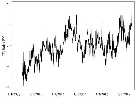
used over the whole sample period (𝑇) for positive and negative words, and the variable’s standard deviation (𝜎).4 _{Figure 2 depicts the course of the FBI constructed with English words for the sample}

period. We can observe the pessimistic atmosphere at the beginning of the financial crisis 2008 and the upward move in the post-crisis era. Overly optimistic movements at the end of 2017/beginning of 2018 might be explained by all-time highs in the stock market, followed by fears of a trade-war between the US and China.

Figure 2: Facebook Index

Course of the modified Facebook Index designed with Google SVI data of English terms since 2008.

4 _{In their paper Siganos et al. (2014) excluded extreme values above the 99th percentile, since some words relate to}

messages with no informative value for people’s sentiment (e.g. „Merry Christmas“). Since the keyword selection in this paper is already narrowed to economic/financial meaning and subjective sentiment, we do not exclude extreme values for the FBI.

14 4.2. VAR model and Granger Causality

In this investigation the hypothesis is that investor attention and sentiment can predict returns. However, it can also be stated that a change in returns cause investor attention and sentiment. Thus, this paper tests statistical causality in the time series for both directions. This paper employs a VAR model to analyze the relationship in a multivariate time-series. Used primarily as a forecasting tool, a basic VAR(p) process is defined as:

( 𝑦_1𝑡 ⋮ 𝑦_𝑣𝑡) = ( 𝑐₁ ⋮ 𝑐_𝑣) + ( 𝜋₁₁1 _{… 𝜋} 1𝑣1 ⋮ ⋱ ⋮ 𝜋_𝑣11 _{… 𝜋} 𝑣𝑣1 ) ( 𝑦_1𝑡−1 ⋮ 𝑦_𝑣𝑡−1) +. . . + ( 𝜋₁₁𝑝 … 𝜋_1𝑣𝑝 ⋮ ⋱ ⋮ 𝜋_𝑣1𝑝 … 𝜋_𝑣𝑣𝑝 ) ( 𝑦1𝑡−𝑝 ⋮ 𝑦_{𝑣𝑡−𝑝}) + ( 𝜀_1𝑡 ⋮ 𝜀_𝑣𝑡) (6)

Where v denotes the number of variables used and p the number of lags. Constants (c) and errors terms (𝜀) are described as vectors. In our analysis we employ a bivariate model, i.e. returns and attention/sentiment, n=2. VAR models can be used to investigate Granger Causality. The model (see Equation 7 and 8) specifies the predictive extent between return (𝑅_𝑡) and search volume 𝑋_𝑡. 𝑋𝑡 denoted as either the search of the index’s names, i.e. ASVI or the sentiment indices, i.e. FEARS

and FBI at week t, using n lags, coefficients 𝜔 and 𝛿 and error term 𝜀.

𝑅_𝑡 = 𝑐₁+ 𝜔_1,1𝑅_𝑡−1+. . . +𝜔_1,𝑛𝑅_𝑡−𝑛+ 𝛿_1,1𝑋_𝑡−1+. . . +𝛿_1,𝑛𝑋_𝑡−𝑛 + 𝜀_𝑡 (7) 𝑋𝑡= 𝑐2+ 𝜔2,1𝑅𝑡−1+. . . +𝜔2,𝑛𝑅𝑡−𝑛+ 𝛿2,1𝑋𝑡−1+. . . +⁡𝛿2,𝑛𝑋𝑡−𝑛+ 𝜀𝑡 (8)

Using an F-Test in (7), the null hypothesis that 𝑋_𝑡 does not Granger Cause 𝑅_𝑡 (𝜔_1,1=…= 𝜔_1,𝑛= 0) is tested. The null hypothesis that 𝑅_𝑡 does not Granger Cause 𝑋_𝑡 (𝛿_2,1=…=⁡𝛿_2,𝑛= 0) is equally conducted with an F-Test in (8).

15

5. Results

Granger Causality Tests and VAR models are powerful and straightforward procedures to examine causality in time series models. Causality in that sense should not be misunderstood and rather be interpreted as precedence. More specifically if x granger causes y it means that x has valuable information for predicting y and might cause y. Both methods require, however, stationary data and are sensitive to the lag length. Too many lags increase the degrees of freedom and might introduce multicollinearity. Too few will on the other hand lead to misspecification. Hence, to test for stationarity, we conduct the Augmented Dickey Fuller test (ADF). To decide on the right lag specification we employ information criteria, namely Akaike- (AIC), Bayesian- (BIC) and Hannan-Quinn information criterion (HQIC).

5.1. Augmented Dickey Fuller Test

The ADF test is a unit-root test to check for stationarity in time series data. The null hypothesis states that the series follows a unit root process, i.e. is nonstationary, against the alternative of no unit root, i.e. stationary time series. Table 1 presents the ADF test without trend component for each index with the specified lags, the test-statistic and p-value. The lag length is selected by choosing the highest lag-specification of the three information criteria stated above. For each index in the observation of investor attention and sentiment except for the FBI with English words, we can reject the hypothesis of nonstationary data at a 1% significance level. For the FBI with English words, we can reject the hypothesis at a 5% significance level. The results confirm that each time series is stationary and hence can be used in the following analysis.

16 Table 1: Augmented Dickey Fuller Test – Stationary Data

This table reports the results of the Augmented Dickey Fuller Test (ADF) for stationary data. The test is conducted on each time series, i.e. proxies of attention (ASVI) and sentiment (FEARS, FBI) for each market (PSI20, DJIA, S&P500) in both language dimensions (EN, PT). The data covers a weekly period from October 2008 – September 2018. The highest lag specification tested on and obtained by information criteria is displayed in the first column, followed by the test-statistic of the ADF. The p-values for the hypothesis of nonstationarity are reported in the last column.

Lags Statistic P-value

ASVI PSI20 7 -9.86 0.00 ASVI DJIA 1 -10.08 0.00 ASVI SP500 1 -10.98 0.00 FEARS PSI20 EN 10 -9.42 0.00 FEARS PSI20 PT 8 -9.84 0.00 FEARS DJIA 7 -10.47 0.00 FEARS SP500 13 -8.37 0.00 FB-Index EN 4 -3.02 0.03 FB-Index PT 6 -4.62 0.00

5.2. Granger Causality Test

Before observing the results of the Granger Causality tests, we explore the information criteria named above to select the appropriate lag-length model. The information criteria would define the optimal variable n in Equation (7) and (8). As can be seen from Table 2, each criterion defines the optimal lag model according to the lowest value relative to the set of alternative models. The optimal model is marked with an underscore. For the analysis we decide on a collection of models using lags back to a quarter year. Table 2, Panel A shows when analyzing causality with the SVI of indices-names, one should specify a model considering last week’s values.

From Panel B and C, it is apparent that the model selection is not as coherent throughout AIC, HQIC and SBIC as in Panel A. However, each criterion is differently computed and in practice has no real superiority over the other. Therefore, the diverging model selections are of no concern, especially as they remain closely together. In the interim we can agree that the optimal model selection lies within a lag-specification of four for each sentiment index. Therefore, Granger Causality tests are presented up to four lags.

17 Table 1: Information Criterion – Optimal lag length

Each panel displays the statistics of the three information criteria, namely Akaike- (AIC), Hannan-Quinn- (HQIC) and Bayesian information criterion (SBIC) for the proxies of attention (ASVI) and sentiment (FEARS, FBI). The results are obtained considering each market, i.e. Portuguese Stock Index (PSI20), Dow Jones Industrial Average (Dow, DJIA) and Standard & Poor’s 500 (SP500, S&P500) for a weekly sample period from October 2008 – September 2018. The maximal lag-length considered in the test is set to 12 weeks. The double underscore indicates the optimal lag model.

Panel A: Attention – ASVI of stock index names

PSI20 Dow SP500

Lags AIC HQIC SBIC AIC HQIC SBIC AIC HQIC SBIC

0 -3.906 -3.899 -3.889 -5.321 -5.315 -5.304 -5.233 -5.227 -5.216 1 -4.020 -4.001 -3.970 -5.939 -5.919 -5.889 -5.557 -5.538 -5.507 2 -4.014 -3.981 -3.930 -5.926 -5.893 -5.842 -5.545 -5.512 -5.461 3 -4.005 -3.959 -3.887 -5.916 -5.870 -5.798 -5.533 -5.487 -5.416 4 -3.997 -3.937 -3.846 -5.914 -5.855 -5.763 -5.528 -5.469 -5.377 5 -4.005 -3.932 -3.820 -5.902 -5.829 -5.717 -5.522 -5.449 -5.337 6 -4.000 -3.914 -3.782 -5.897 -5.811 -5.679 -5.508 -5.422 -5.290 7 -3.998 -3.900 -3.747 -5.884 -5.786 -5.633 -5.495 -5.396 -5.243 8 -3.987 -3.875 -3.702 -5.894 -5.782 -5.609 -5.508 -5.396 -5.223 9 -3.976 -3.851 -3.657 -5.891 -5.766 -5.572 -5.510 -5.385 -5.191 10 -3.968 -3.830 -3.616 -5.884 -5.746 -5.531 -5.507 -5.369 -5.155 11 -3.965 -3.814 -3.579 -5.868 -5.717 -5.482 -5.500 -5.348 -5.114 12 -3.955 -3.790 -3.535 -5.856 -5.691 -5.436 -5.509 -5.345 -5.090 Panel B: Sentiment - FEARS

PSI20 - EN PSI20 - PT DJIA S&P500

Lags AIC HQIC SBIC AIC HQIC SBIC AIC HQIC SBIC AIC HQIC SBIC 0 -3.73 -3.72 -3.71 -4.12 -4.12 -4.11 -4.48 -4.47 -4.46 -4.39 -4.39 -4.38 1 -3.77 -3.75 -3.72 -4.23 -4.21 -4.18 -4.53 -4.51 -4.48 -4.44 -4.42 -4.39 2 -3.86 -3.83 -3.78 -4.27 -4.23 -4.18 -4.60 -4.57 -4.52 -4.52 -4.49 -4.44 3 -3.92 -3.87 -3.80 -4.27 -4.22 -4.15 -4.67 -4.63 -4.56 -4.58 -4.53 -4.46 4 -3.92 -3.86 -3.77 -4.26 -4.21 -4.11 -4.71 -4.65 -4.56 -4.62 -4.56 -4.47 5 -3.91 -3.84 -3.73 -4.26 -4.19 -4.08 -4.70 -4.63 -4.52 -4.61 -4.54 -4.43 6 -3.90 -3.81 -3.68 -4.25 -4.17 -4.04 -4.69 -4.61 -4.47 -4.61 -4.52 -4.39 7 -3.89 -3.79 -3.64 -4.24 -4.14 -3.99 -4.70 -4.60 -4.45 -4.62 -4.52 -4.37 8 -3.88 -3.77 -3.59 -4.24 -4.13 -3.96 -4.69 -4.58 -4.41 -4.63 -4.52 -4.34 9 -3.87 -3.74 -3.55 -4.23 -4.10 -3.91 -4.69 -4.56 -4.37 -4.62 -4.50 -4.31 10 -3.86 -3.72 -3.51 -4.22 -4.08 -3.87 -4.69 -4.55 -4.34 -4.63 -4.49 -4.28 11 -3.85 -3.70 -3.47 -4.22 -4.07 -3.83 -4.68 -4.53 -4.30 -4.62 -4.47 -4.24 12 -3.84 -3.68 -3.43 -4.20 -4.04 -3.79 -4.67 -4.51 -4.26 -4.61 -4.45 -4.20

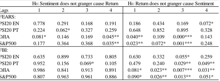
18 For Granger Causality, Table 3 and Table 4 illustrate the results of the F-Test on Equation (7) and Equation (8) on the left and right panel respectively. Each column determines the lags used, i.e. the selection of n. The displayed numbers are p-values. P-values below a defined significance level (1%, 5% and 10%) deduce the rejection of the respective null-hypothesis of no Granger Causality. Hence, we can conclude from Table 3 that the Hypothesis of no Granger Causality cannot be rejected regardless which market index name was searched. Thus, those SVI do not granger cause returns. On the other hand, past returns reveal predictive information about current search inquiries for “Dow” and “SP500” using each lag-model but not for “PSI20”. Henceforth, the data returns unidirectional causality from returns to SVI in most lags. The difference in regions is not surprising since return movements in large markets like the DJIA and S&P500 arouse more attention and search action for those indices worldwide. Because of the smaller size of the Portuguese market we presuppose that higher search activity for the PSI20 caused by return movements in that index is rather unlikely.

Panel C: Sentiment - FBI

PSI20 - EN PSI20 - PT DJIA S&P500

Lags AIC HQIC SBIC AIC HQIC SBIC AIC HQIC SBIC AIC HQIC SBIC 0 -2.48 -2.47 -2.46 -3.28 -3.27 -3.26 -3.11 -3.11 -3.10 -3.01 -3.00 -2.99 1 -3.56 -3.54 -3.51 -3.71 -3.69 -3.66 -4.20 -4.18 -4.15 -4.09 -4.07 -4.04 2 -3.64 -3.61 -3.55 -3.78 -3.74 -3.69 -4.27 -4.24 -4.19 -4.17 -4.13 -4.08 3 -3.66 -3.61 -3.54 -3.80 -3.75 -3.68 -4.28 -4.24 -4.17 -4.18 -4.13 -4.06 4 -3.68 -3.62 -3.53 -3.80 -3.74 -3.65 -4.32 -4.26 -4.17 -4.21 -4.15 -4.06 5 -3.67 -3.59 -3.48 -3.80 -3.73 -3.62 -4.31 -4.23 -4.12 -4.20 -4.13 -4.02 6 -3.66 -3.57 -3.44 -3.80 -3.72 -3.58 -4.30 -4.21 -4.08 -4.20 -4.11 -3.98 7 -3.66 -3.56 -3.41 -3.79 -3.69 -3.54 -4.29 -4.19 -4.04 -4.19 -4.09 -3.94 8 -3.65 -3.54 -3.37 -3.78 -3.67 -3.50 -4.29 -4.17 -4.00 -4.19 -4.08 -3.91 9 -3.65 -3.52 -3.33 -3.77 -3.65 -3.46 -4.30 -4.18 -3.98 -4.21 -4.09 -3.89 10 -3.66 -3.52 -3.31 -3.76 -3.63 -3.41 -4.30 -4.16 -3.95 -4.21 -4.08 -3.87 11 -3.65 -3.50 -3.26 -3.76 -3.61 -3.38 -4.29 -4.14 -3.91 -4.21 -4.06 -3.82 12 -3.64 -3.48 -3.23 -3.75 -3.58 -3.33 -4.29 -4.13 -3.88 -4.21 -4.05 -3.80

19 Table 3: Granger Causality Test – Attention

This table displays the p-values for bilateral Granger Causality tests on investor attention and stock index returns. Adjusted Google Search volume data (ASVI) is used to proxy investor attention. The stock indices include the Portuguese stock index (PSI20), the Dow Jones Industrial Average (DJIA) and Standard & Poor’s 500 index (S&P500). The data on ASVI and return covers a weekly sample period from October 2008 – September 2018. The results refer to the null-hypothesis (H0) from both directions reported in the right and left panel, respectively. The columns include

the results on lag-specifications from 1 to 4 weeks. Significance at the 1%, 5% and 10%-level is denoted by ***, **, *, respectively.

The more striking result to emerge from the data is the unilateral relation. In contrast to Vozlyublennaia (2014), who detected significant change in returns following a raise in SVI for the DJIA- and S&P500 index from 2004 to 2012, no such result is apparent with data from 2008 to 2018. This finding may either suggest that the former paper was deducted on a different data basis or that the markets prove to be efficient. For the former one could argue that Google might have changed its database or calculation for SVI significantly after 2012, or that the use of ln(SVI) as opposed to the use of ASVI in this paper drives the different results. For the latter on the other side, one could consider the theoretical model of Grossman and Stiglitz (1980) in which more informed agents, resulting from e.g. increasing attention, leads to informed prices and subsequently markets becoming more efficient.

The results obtained from the Granger Causality test on investor sentiment are set out in Table 4. Again, strong evidence was found that returns granger cause sentiment obtained through SVI. Observing FEARS index and FBI, various lag specifications show significant causality findings. For example, lag 4 for the FEARS index on PSI20 return suggests significant results at a 10% significance level and each lag-model for the FBI on US market returns shows significant to highly

Lags 1 2 3 4 1 2 3 4

ASVI:

PSI20 0.643 0.827 0.880 0.646 0.403 0.928 0.991 0.995

Dow 0.802 0.235 0.503 0.371 0.000*** 0.000*** 0.000*** 0.000***

SP500 0.389 0.676 0.781 0.747 0.000*** 0.001*** 0.002*** 0.001***

20 significant results. In a way this outcome is not unanticipated. Undoubtedly, high/low returns in the market affect investor sentiment.

Table 4: Granger Causality Test – Sentiment

This table displays the p-values for bilateral Granger Causality tests on investor sentiment and stock index returns. Google Search volume data is used to construct two sentiment indices, FEARS and FBI for which results are reported in the top and bottom panel, respectively. The stock indices include the Portuguese stock index (PSI20), the Dow Jones Industrial Average (DJIA) and Standard & Poor’s 500 index (S&P500). Each sentiment index is further constructed with English (EN) and Portuguese (PT) terms for the tests on the PSI20. The data on sentiment and return covers a weekly sample period from October 2008 – September 2018. The results refer to the null-hypothesis (H0) from both

directions reported in the right and left panel, respectively. The columns include the results on lag-specifications from 1 to 4 weeks. Significance at the 1%, 5% and 10%-level is denoted by ***, **, *, respectively.

More interestingly is the left-side panel. In theory we assumed that sentiment might predict future returns. Examining the FEARS sentiment index, this theory holds true for both the American market and the FEARS index constructed with Portuguese words for the PSI20, but not the one constructed with English words. The different outcomes in the PSI20 would suggest that the sentiment of Portuguese speaking investors induces market movements rather than international investor sentiment. Since the PSI20 is probably considered more by the former investors, the derived results are plausible. Conclusively in that sense, last month’s sentiment for example may reveal information about the future movement of the DJIA and S&P500 today. Similarly, the sentiment of Portuguese speaking investors of two weeks ago might predict returns today.

Lags 1 2 3 4 1 2 3 4 FEARS: PSI20 EN 0.778 0.291 0.168 0.191 0.186 0.434 0.169 0.072* PSI20 PT 0.224 0.062* 0.327 0.259 0.648 0.852 0.895 0.328 DJIA 0.081* 0.146 0.169 0.045** 0.040** 0.109 0.000*** 0.143 S&P500 0.177 0.364 0.368 0.035** 0.023** 0.072* 0.001*** 0.248 FBI: PSI20 EN 0.635 0.899 0.733 0.805 0.630 0.332 0.055* 0.259 PSI20 PT 0.952 0.156 0.069* 0.105 0.479 0.240 0.029** 0.049** DJIA 0.986 0.841 0.913 0.891 0.081* 0.023** 0.007*** 0.031** S&P500 0.807 0.963 0.961 0.886 0.090* 0.026** 0.013** 0.051*

21 In the robustness test with the FBI, however, these results are not backed up for the American market (see Table 4). No statistically significant precedence was detected in that region. Nonetheless, evidence of sentiment index granger causing Portuguese market returns was found for the FBI constructed with Portuguese words under a significance level of 10% in the third lag. Equivalently to the FEARS index, no such result is achieved with an FBI constructed with English words. The right panel of Table 4 further indicates anew that returns granger cause sentiment movement with significance levels up to 1%.

Ultimately, the lag indication from the significant Granger Causality tests for investor sentiment corresponds to the optimal model selection by the information criteria. For the FEARS index the second lagged week is supported as an optimal lag-length indication by HQIC and SBIC (Table 2, Panel B). Likewise, the third lagged week in the test for the FBI reassures the optimal lag-length model looking at HQIC (Table 2, Panel C). In conclusion, only the sentiment indices constructed with Portuguese words present reliable forecasting ability for returns in the Portuguese market. The results in the different regions might point to the size of the market indices used. For the firm level in the cross section, it is argued that sentiment is especially related to stocks held by noise traders (Lee et al., 1991). Compared to institutional investors, noise traders might consider smaller firms to a greater extent, therefore stock returns of small companies are more exposed to behavioral biases (Baker and Wurgler, 2007; Lemmon and Portniaguina, 2006). This concept might be adopted to the market level in this analysis. Accordingly, the significant results of Granger Causality in the Portuguese market can be traced back to a high proportion of noise traders in the PSI20. However, this interpretation must be further tested in the future, as the theory relates to the individual stock level.

22

5.3. VAR model

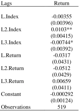
With the Granger Causality results, we can establish a VAR model with the optimal lag-length. Different to a Granger Causality test, the VAR model returns the proper estimators to derive a forecasting equation. In the following we refer to the VAR model using the ‘FBI PSI20 PT’, since it shows a required feedback relationship, i.e. Granger Causality was found on both panel sides. Our main interest is the prediction of returns, for which the regression of the VAR-equation is summarized in Table 5.

Table 5: VAR model FBI PSI20 PT

This table provides VAR estimation results for Portugal Stock Index returns (Return) on lagged values of the sentiment index (Index) and the stock returns itself. The sentiment index refers to the Facebook Index constructed with Google search volume of Portuguese terms. The data on returns and search volume covers a weekly sample period from October 2008 – September 2018. The two VAR specifications enclose 3 lags. Reported coefficients are followed by standard errors in parentheses. Significance at the 1%, 5% and 10%-level is denoted by ***, **, *, respectively.

Lags Return L.Index -0.00355 (0.00396) L2.Index 0.0103** (0.00415) L3.Index -0.00744* (0.00392) L.Return -0.0317 (0.0431) L2.Return -0.0512 (0.0429) L3.Return 0.00659 (0.0411) Constant -0.000292 (0.00124) Observations 519

It is apparent from the table above that PSI20 return is negatively influenced by positive sentiment experienced three weeks ago, showing significance at the 10%-level. In the same way, return is positively influenced by sentiment observed two weeks ago at the 5% significance level. Ultimately, from the data we cannot certainly support the hypothesis of De Long et al. (1990) that

23 returns revert to fundamental value since our estimates show different signs5. However, the fact that our estimates are significant, and the result of Granger Causality do acknowledge the forecasting potential.

6. Discussion

Despite the fact that our results provide new insights into the relation between returns and attention/sentiment especially in the Portuguese market, they should be seen with caution. As described, Google SVI data is somewhat opaque. Non-transparence and no time-continuing datasets limit the preciseness of results. Furthermore, we cannot accurately check the information obtained from the search request as well as who exactly is googling. However, it should be noted that neither news analysis nor surveys capture the ‘real’ sentiment or attention of investors. From an academic perspective, reproducibility is another caveat. The basis of the calculation of SVI changes constantly, hence SVI gathered today does not equal SVI gathered yesterday. We further observed that for the analysis of non-English markets it is important to examine the language dimension. However, this is challenging owing to different ascriptions in the meanings of keywords. Our dictionary mainly contains general terms, like ‘gold’ and ‘depression’, but we cannot exclude the possibility of missing or incorrectly assigning Portuguese-specific sentiment terms with a simple translation. Another crucial concern is that search inquiries and expected future returns might rather be increasing simultaneously because of macroeconomic events and conditions. To control for those, one could use several macroeconomic variables. Da et al. (2015) included in their analysis the ADS index, a daily measurement of American economic condition including payroll employment, GDP and jobless claims created by Aruoba et al. (2009). In addition,

5 _{Additionally, analyzing structural shocks through (orthogonalized) Impulse Response Functions did not show}

24 they adopt the Policy Uncertainty Index by Baker et al. (2013) which counts macroeconomic related news in U.S. newspaper. Since those indices are not yet available for the Portuguese economy, they could not be included in our analysis.

7. Conclusion

With Google Volume Search data, we attempt to proxy investor attention and sentiment to investigate the relation to returns in the US and Portuguese stock market. We hypothesized that either may have valuable information for the prediction of future returns. The search amount of the index’s names, that is investor attention, did not show significant Granger Causality. To examine investor sentiment forecasting ability, we composed two sentiment indices, FBI and FEARS index with the SVI of a set of positive and negative connoted terms. The FEARS index is already known to employ SVI data, hence we designed the modified Facebook Happiness Index, i.e. FBI for robustness purposes. For both countries no significant precedence was found, which suggests no predictive capability. However, the analysis was altered by using Portuguese terms instead of English ones to adjust for the language dimension. We observe that for both FEARS and FBI ‘Portuguese’ sentiment show significant forecasting information for the returns in the Portuguese stock market.

Conclusively, one could state that in case of investor attention, SVI reveals no additional information, pointing to market efficiency. The analysis of sentiment on the other side still suggests irrational investor behavior. SVI data seems to contain information about returns of the Portuguese stock market, whereas the US market has adjusted to efficiently incorporate any. Nonetheless, it is substantial to control for macroeconomic conditions to complement the analysis. Google Search data comes with caveats and should be cautiously interpreted as a proxy of investor attention and sentiment. Future research on the relation between attention/sentiment and stock returns could

25 focus on machine learning approaches, e.g. word embedding with deep neural networks (Peng and Jiang, 2016) or the examination of professional investors by e.g. analyzing Bloomberg news.

References

Aouadi, A., Arouri, M., & Teulon, F. (2013). Investor attention and stock market activity: Evidence from France. Economic Modelling, 35, 674–681.

Aruoba, S. B., Diebold, F. X., & Scotti, C. (2009). Real-time measurement of business conditions. Journal of Business & Economic Statistics, 27, 417–427.

Baker, M., & Wurgler, J. (2006). Investor sentiment and the cross-section of stock returns. The Journal of Finance, 61, 1645–1680.

Baker, M., & Wurgler, J. (2007). Investor sentiment in the stock market. Journal of Economic Perspectives, 21, 129–151.

Baker, M., Wurgler, J., & Yuan, Y. (2012). Global, local, and contagious investor sentiment. Journal of Financial Economics, 104, 272–287.

Baker, S. R., Bloom, N., & Davis, S. J. (2013). Measuring economic policy uncertainty. Working Paper, Stanford University.

Bank, M., Larch, M., & Peter, G. (2011). Google search volume and its influence on liquidity and returns of German stocks. Financial Markets and Portfolio Management, 25, 239–264. Barber, B. M., & Odean, T. (2008). All that glitters: the effect of attention and news on the buying

behavior of individual and institutional investors. Review of Financial Studies, 21, 785–818. Bijl, L., Kringhaug, G., Molnár, P., & Sandvik, E. (2016). Google searches and stock returns.

International Review of Financial Analysis, 45, 150–156.

Challet, D., & Bel Hadj Ayed, A. (2014). Do google trend data contain more predictability than price returns? SSRN Electronic Journal. doi:10.2139/ssrn.2405804

Chemmanur, T. J., & Yan, A. (2009). Advertising, attention, and stock returns. SSRN Electronic Journal. doi:10.2139/ssrn.1340605

Da, Z., Engelberg, J., & Gao, P. (2011). In search of attention. The Journal of Finance, 66, 1461– 1499.

Da, Z., Engelberg, J., & Gao, P. (2015). The sum of all fears investor sentiment and asset prices. Review of Financial Studies, 28, 1–32.

De Long, J. B., Shleifer, A., Summers, L. H., & Waldmann, R. J. (1990). Noise trader risk in financial markets. Journal of Political Economy, 98, 703–738.

Dimpfl, T., & Jank, S. (2016). Can internet search queries help to predict stock market volatility? : search queries and market volatility. European Financial Management, 22, 171–192.

Engelberg, J. E., & Parsons, C. A. (2011). The causal impact of media in financial markets. The Journal of Finance, 66, 67–97.

26 Fink, C., & Johann, T. (2014). May i have your attention, please: the market microstructure of investor attention (SSRN Scholarly Paper No. ID 2139313). Rochester, NY: Social Science Research Network. Retrieved from https://papers.ssrn.com/abstract=2139313

Goddard, J., Kita, A., & Wang, Q. (2015). Investor attention and FX market volatility. Journal of International Financial Markets, Institutions and Money, 38, 79–96.

Grossman, S. J., & Stiglitz, J. E. (1980). On the Impossibility of Informationally Efficient Markets. The American Economic Review, 70(3), 393-408.

Grullon, G., Kanatas, G., & Weston, J. P. (2004). Advertising, breadth of ownership, and liquidity. Review of Financial Studies, 17, 439–461.

Gwilym, O. ap, Hasan, I., Wang, Q., & Xie, R. (2012). In search of concepts: returns, trading volume and speculative demand. SSRN Electronic Journal. doi:10.2139/ssrn.2062813

Huang, D., Jiang, F., Tu, J., & Zhou, G. (2015). Investor sentiment aligned: a powerful predictor of stock returns. Review of Financial Studies, 28, 791–837.

Huang, M. Y., Randall R. R., Convery P. D. (2017). Modeling Stock Market Movements using Google Trend Searches. Article from the Department of Economics - University of California, Los Angeles. Retrieved from: https://melodyyhuang.github.io/

Jiang, F., Lee, J., Martin, X., & Zhou, G. (2018). Manager sentiment and stock returns. Journal of Financial Economics. In Press

Joseph, K., Babajide Wintoki, M., & Zhang, Z. (2011). Forecasting abnormal stock returns and trading volume using investor sentiment: Evidence from online search. International Journal of Forecasting, 27, 1116–1127.

Kahneman, D. (1973). Attention and effort. Englewood Cliffs, N.J: Prentice-Hall.

Kearney, C., & Liu, S. (2014). Textual sentiment in finance: A survey of methods and models. International Review of Financial Analysis, 33, 171–185.

Kim, N., Lučivjanská, K., Molnár, P., & Villa, R. (2018). Google searches and stock market activity: Evidence from Norway. Finance Research Letters. doi:10.1016/j.frl.2018.05.003 Kim, Y. H. (Andy), & Meschke, F. (2011). Ceo interviews on cnbc. SSRN Electronic Journal.

doi:10.2139/ssrn.1745085

Lee, C. M. C., Shleifer, A., & Thaler, R. H. (1991). Investor sentiment and the closed-end fund puzzle. The Journal of Finance, 46, 75–109.

Lemmon, M., & Portniaguina, E. (2006). Consumer confidence and asset prices: some empirical evidence. Review of Financial Studies, 19, 1499–1529.

Merton, R. C. (1987). A simple model of capital market equilibrium with incomplete information. The Journal of Finance, 42, 483–510.

Peng, Y., & Jiang, H. (2016). Leverage financial news to predict stock price movements using word embeddings and deep neural networks. In Proceedings of the 2016 Conference of the North American Chapter of the Association for Computational Linguistics: Human Language Technologies (S. 374–379). San Diego, California: Association for Computational Linguistics. Preis, T., Moat, H. S., & Stanley, H. E. (2013). Quantifying trading behavior in financial markets

27 Preis, T., Reith, D., & Stanley, H. E. (2010). Complex dynamics of our economic life on different scales: insights from search engine query data. Philosophical Transactions of the Royal Society A: Mathematical, Physical and Engineering Sciences, 368, 5707–5719.

Risteski, D., & Davcev, D. (2014). Can We Use Daily Internet Search Query Data to improve Predicting Power of EGARCH Models for Financial Time Series Volatility? International conference on Computer Science and Information Systems.

Sibley, S. E., Wang, Y., Xing, Y., & Zhang, X. (2016). The information content of the sentiment index. Journal of Banking & Finance, 62, 164–179.

Siganos, A., Vagenas-Nanos, E., & Verwijmeren, P. (2014). Facebook’s daily sentiment and international stock markets. Journal of Economic Behavior & Organization, 107, 730–743. Takeda, F., & Wakao, T. (2014). Google search intensity and its relationship with returns and

trading volume of Japanese stocks. Pacific-Basin Finance Journal, 27, 1–18.

Tantaopas, P., Padungsaksawasdi, C., & Treepongkaruna, S. (2016). Attention effect via internet search intensity in Asia-Pacific stock markets. Pacific-Basin Finance Journal, 38, 107–124. Tetlock, P. C., Saar-Tsechansky, M., & Macskassy, S. (2008). More than words: quantifying

language to measure firms’ fundamentals. The Journal of Finance, 63, 1437–1467.

Vlastakis, N., & Markellos, R. N. (2012). Information demand and stock market volatility. Journal of Banking & Finance, 36, 1808–1821.

Vozlyublennaia, N. (2014). Investor attention, index performance, and return predictability. Journal of Banking & Finance, 41, 17–35.

Appendix

Appendix 1: Augmented Dickey Fuller Test – Attention lnSVI

This table reports the results of the Augmented Dickey Fuller Test (ADF) for stationary data. The test is conducted on the time series of investor attention using logarithm search volume (lnSVI). The data covers a weekly period from October 2008 – September 2018. The highest lag specification tested on and obtained by information criteria is displayed in the first column, followed by the test-statistic of the ADF. The p-values for the hypothesis of no-stationarity are reported in the last column.

Lags Statistic P-value PSI20 lnSVI 4 -6.29 0.00 DJIA lnSVI 7 -3.11 0.10 SP500 lnSVI 8 -2.29 0.44

28 Appendix 2: Granger Causality Test – Sentiment – Extended List

This table displays the p-values for bilateral Granger Causality tests on investor sentiment and stock index returns. Google Search volume data of an extended list of terms is used to construct the FEARS sentiment index. The stock indices include the Portuguese stock index (PSI20), the Dow Jones Industrial Average (DJIA) and Standard & Poor’s 500 index (S&P500). The data on sentiment and return covers a weekly sample period from October 2008 – September 2018. The results refer to the null-hypothesis (H0) from both directions reported in the right and left panel, respectively.

The columns include the results on lag-specifications from 1 to 4 weeks. Significance at the 1%, 5% and 10%-level is denoted by ***, **, *, respectively.

Appendix 3: Impulse Response Function

Impulse Response Function under Cholesky Decomposition, showing a structural shock of the FBI with Portuguese words (Index) on the returns of PSI20 (Return)

Lags 1 2 3 4 1 2 3 4

FEARS:

PSI20 0.85 0.97 0.34 0.49 0.15 0.48 0.70 0.31

DJIA 0.11 0.28 0.05* 0.24 0.41 0.55 0.00*** 0.11

SP500 0.24 0.57 0.34 0.25 0.45 0.65 0.03** 0.32