M
ASTER
M
ONETARY AND
F
INANCIAL
E
CONOMICS
M
ASTER
´
S
F
INAL
W
ORK
D
ISSERTATION
T
HE
D
ETERMINANTS OF
S
OVEREIGN
B
OND
Y
IELD
S
PREADS IN THE
EMU
Y
ULIYA
S
HEVCHUK
M
ASTER
M
ONETARY AND
F
INANCIAL
E
CONOMICS
M
ASTER
´
S
F
INAL
W
ORK
D
ISSERTATION
T
HE
D
ETERMINANTS OF
S
OVEREIGN
B
OND
Y
IELD
S
PREADS IN THE
EMU
Y
ULIYA
S
HEVCHUK
S
UPERVISION:
A
NTÓNIOA
FONSO0
To my family, without whom none of my success would be possible.
i ABSTRACT
A panel dataset of euro area countries was used to assess the determinants of sovereign bond yield spreads from first quarter of 1995 to the last quarter of 2017. In the period before the financial crisis, the government bond yield spreads were mostly determined by the expected debt to GDP, the credit risk factor and economic growth. With the eruption of the financial crisis, the analysis suggests that markets have started to take into consideration more fundamentals to determine the price of government bond yield spreads, such as liquidity risk and international risk. It was also concluded that there is a difference between the determinants of the government bond yield spread of core and periphery group.
JEL: C23, F34, G01, H50.
ii TABLE OF CONTENTS
Abstract ... i
Table of Contents... ii
Table of Figures ... iii
Acknowledgments ... iv
1. Introduction ... 1
2. Related literature ... 3
3. Analysis ... 7
3.1 Methodology ... 7
3.2 Data and stylized facts ... 9
3.3 Measuring core-periphery effect ... 15
3.4 Panel estimation results ... 18
4. Conclusion ... 22
References ... 23
iii TABLE OF FIGURES
FIGURE 1 - 10-years government bond yield spread………...….……10
FIGURE 2 - German 10-year government bond yield and VIX...…...11
FIGURE 3: Expected budget balance as percentage of GDP………..12
FIGURE 4: Expected debt as percentage of GDP……….13
FIGURE 5: Average credit ratings………...14
iv ACKNOWLEDGMENTS
I would like to express my deepest gratitude to Professor Antonio Afonso, for the guidance, the support and the good words and the patience towards this project. For every lesson, advice and problem solving.
To Alexandre Correia da Silva and Mayara Cabral for the precious advices in each stage of the project, your aid, motivation and optimism, I thank you.
To BNP Paribas and Transversal Control team (Manuel Pilo and Victoria Braniste). I am grateful for the excellent work environment and comprehension from your side.
Moreover, a special gratitude to my parents, Tetyana and Oleg, and my brother, Daniel, because I owe it all to you.
1 1.INTRODUCTION
The Economic and Monetary Union (EMU), in January of 1999, brought to life an integrated market, with no visible currency risk and closer coordination of monetary policies across euro countries. Due to this union, the public bonds issued by different Euro-area governments were considered by many investors as close substitutes. This perception originated a significant decrease in the interest spread of 10-year government bonds against the benchmark, the German bonds, converging between the member countries in less than a year after the introduction of EMU. Yet, market participants have never regarded bonds issued by euro-area Member States as perfect substitutes. Differences in yield levels across countries have indeed remained to different extents for different issuers and maturities, and became more sizable during the course of 2008 and 2009.
The global financial turmoil began in mid-2007, and reached its first climax in September 2008, with the collapse of Lehman Brothers. Fiscal imbalances expanded in most European Economies, with several countries breaking the rules of the Stability and Growth Pact, facing excessive deficits for a prolonged period. At the end of 2008, a sudden rise in bond spreads relative to Germany was observed for many economies. In October 2008, the spread reached an unprecedented level, being higher than 100 basis points for the first time. The lack of a strong market reaction in the wake of these adverse fiscal developments has prompted people to argue that the euro and the ongoing process of financial integration have eliminated markets’ ability or willingness to discriminate the quality of national fiscal policies (Manganelli and Wolwijk, 2007). In times of heightened financial and economic uncertainty, investors typically have a higher preference for less risky and liquid assets, thereby increasing the premium for risky assets as portfolio composition is adjusted to the desired new equilibrium (Favero et al., 20011). If we have market discipline the government has the incentive to present solid economic indicators, otherwise markets will most likely penalize it, demanding higher yields. Governments have therefore to take into account these higher financing costs when planning their fiscal policies. Ceteris paribus, strong market discipline does not encourage governments to take unbalanced fiscal policies, promoting as a result fiscal discipline.
2
This unprecedented surge in the concerns of financial markets about some governments’ capacity to meet their future debt obligations leads to the importance to determine what causes the fluctuations of the government bond yield spreads. In addition to a higher cost of borrowing, the increase in sovereign bond yield spreads may reflect the fact that investors are less willing to provide funding to sovereign borrowers. Therefore, governments might lose the ability to access capital markets.
Based on the finding of this study, it can be concluded that in the period before the financial crisis the government bond yield spreads were mostly determined by the expected debt to GDP, the credit risk factor and economic growth.
With the eruption of the financial crisis, the analysis suggests that markets have started to take into consideration more fundamentals to determine the price of government bond yield spreads. International risk and the liquidity risk were two indicators that started to have a meaningful influence on spreads after 2009. Fiscal determinants, credit risk were also significant for this model. The average credit ratings while is significant in spread determination, after 2009 have unexpected relationship, presenting a positive sign.
The remaining of the paper is organized as follows. Section two reviews the related literature on the determinants of the euro area sovereign spreads before and during the European debt crisis. Section three presents and discusses the data, methodology and empirical results. Section four concludes.
3 2.RELATED LITERATURE
In the European Monetary Union, given the single monetary policy, no exchange rate risk and the relative integration of the national bond market, the general literature use three main variables as the determinants of long-term sovereign yield spreads: the international risk factor, credit risk and the liquidity risk.
The international risk factor captures the level of perceived risk and its unit price. The empirical evidence shows that a higher (lower) value of international risk factor tends to cause an increase (reduction) in the government bond spread. This is empirically approximated using the indexes of the US stock market implied volatility or the spread between the yields of the corporate bonds against US treasury bills (Afonso et al., 2018, Hui and Chung, 2011, Beber et al., 2009).
The second explanatory factor, the credit risk, refers to the risk of the issuer´s default, who may no longer be able to pay interest or/and pay back the capital. It is linked to the sustainability of the fiscal position. Therefore, in terms of credit risk, sovereign bond yield spreads should be related to each country´s public finances sustainability indicators. It is expected that higher (lower) value of credit risk increases (decreases) the government bond spread. An extensive literature has indeed concluded that markets tend to attach additional risk to the loosening of the fiscal position of the country (see e.g. Afonso and Rault, 2010, Schuknecht et al., 2010)
Liquidity risk is another important variable that must be taken into consideration to understand the government bond yields. It refers to the risk of selling less liquid assets at worse market conditions (higher transaction costs, greater price impact) than more liquid ones. This variable provides therefore an indication of the depth of the sovereign bond market. Liquidity is particularly difficult to measure empirically, usually approximated using bid-ask spreads, transaction volumes and the level of or the share of a country’s debt in global/EMU-wide sovereign debt (see e.g. Favero et al., 2010, Arghyrou and Kontonikas, 2011).
The literature on the EMU government bonds covering the period prior to the global financial crisis is not unanimous regarding the role of each of the three main determinants discussed above. However, the prevailing views can be summarized as follows: First, the international risk factor was important to determine spreads against Germany (see
4
Codogno et al., 2003; Favero et al., 2010, Manganelli and Wolswijk, 2007). This effect was particularly strong during periods of tightening international financial conditions (e.g. excessive current account) (see Barrios et al., 2009) as well as for countries with high levels of public debt (see Codogno et al., 2003). As Hui and Chung, (2011) show, the VIX index explains an additional 4.3% of the implied volatility; however, it is only marginally significant. As per Arghyrou and Kontonikas, (2011), VIX is not significant as a determinant of spreads in any country, thereby suggesting a weak link between spreads and global financial risk during the pre-crisis period.
Second, credit risk was significant determinant of the government bond yield spread, as suggested by Bernoth et al. (2004), Manganelli and Wolswijk, (2007) and Gerlach et al. (2010). Bernoth and Wolff, (2008) and Schuknecht et al. (2010) interpret these findings as evidence that the Stability and Growth Pact was a credible mechanism imposing fiscal discipline among EMU members. The Pact might reduce monitoring by financial markets of fiscal developments if market participants are confident that peer pressure and sanctions will lead governments to reduce the budgetary position. Any excess over 3% of GDP would only be considered as a temporary concern, not giving rise to a major disruption in the financial markets. Manganelli and Wolswijk, (2007), find that the penalties imposed by markets were insufficiently high to encourage EMU governments to change unsustainable fiscal policies.
Finally, there is a controversial opinion on the role played by liquidity. On the one hand, Bernoth et al. (2004) and Schuknecht et al. (2010) conclude that liquidity is not a significant determinant of the sovereign yield spread in euro area countries. Codogno et al. (2003) and Arghyrou and Kontonikas, (2011) also indicate a very limited effect of liquidity. On the other hand, Pagano and Von Thadden, (2004), Jankowitsch et al. (2002) Gomez-Puig, (2006) and Beber et al. (2009) argue in favor of a more prominent liquidity effect. Liquidity effects are found to be higher during periods of tightening financial conditions as the potential cost associated with investing in an illiquid, creditworthy asset is higher than the cost associated with investing in a liquid, yet less creditworthy asset during volatile market periods (Beber et al., 2009). In contrast, Favero et al. (2010) finds that during periods of high aggregate risk the effect of liquidity on yield differentials is not significantly different from zero.
5
When it comes to the crisis period, there is a broad consensus in the literature that the observed widening of the EMU spreads is mainly driven by the increase of global risk factor. In this process, the role of domestic banking sectors is crucial, as suggested by Gerlach et al. (2010) and Acharya et al. (2011). Global banking risk has been transformed into sovereign risk as shortages in banking liquidity restricted credit to the private sector causing economic recession and increasing fiscal imbalances.
With national banking sectors having different degrees of exposure to global financial conditions, the increase in the global risk factor causes a heterogeneous impact on national spreads. Gerlach et al. (2010), Schuknecht et al. (2010) and Hui and Chang (2011) among others, established the importance of the global risk factor during the crisis period and its impact on the latter through the financial sector. Haugh and others (2009) have shown that the effects of fiscal variables on yield spreads are likely to be amplified through their interaction with risk aversion.
Beber and others (2009), Manganelli and Wolswijk, (2007), Afonso et al. (2018) and Arghyrou et al. (2011) find that liquidity is a significant variable in explaining spreads and that the liquidity premiums tend to be high when interest rates are high. As per Barrios et al. (2009) liquidity played a role in explaining the evolution of yield spread for the majority of countries, but in spite of the strong deterioration in the liquidity condition in the Austrian and Portuguese government bond market in the crisis period, the liquidity variable is not significant.
In the research carried out by Barbosa and Costa (2010), they found that the influence of credit risk and liquidity premiums augmented both in absolute terms in the period following the bankruptcy of Lehman Brothers. Between January 2007 and August 2008, the increase in spreads was determined by enhanced risk aversion in financial markets. In the months following the bankruptcy of Lehman Brothers, the risk premium in financial markets continued to contribute to a widening of spreads, although it was no longer the main factor behind the changes in spreads. During that period, most countries witnessed a significant raise in the liquidity premium and, to a lesser extent, in the credit risk premium. Credit risk and liquidity are relative concepts, particularly in the context of flight-to-quality and flight-to-liquidity. Indeed, an investor considering shifting funds
6
from one asset to another necessarily has to take into account the relative credit quality and liquidity of the two assets at a point in time (Beber et al., 2009).
7 3.ANALYSIS
3.1 Methodology
The dependent variable of the model is the 10-year government bond yield spread versus Germany, , where i presents the 10 countries of the model and t is the specific period.
(1) 𝑠𝑝𝑟𝑖𝑡 = 𝛽0+ 𝛽1𝑠𝑝𝑟𝑖𝑡−1+ 𝛽2𝑣𝑖𝑥𝑡+ 𝛽3𝑙𝑖𝑞𝑖𝑡+ 𝛽4𝑏𝑎𝑙𝑎𝑛𝑐𝑒𝑖𝑡+ 𝛽5𝑑𝑒𝑏𝑡𝑖𝑡+ 𝛽6𝑒𝑥𝑟𝑡𝑖𝑡+ 𝛽7𝑖𝑛𝑑𝑝𝑟𝑖𝑡+ 𝜀𝑖𝑡
Following Afonso et al. (2015), to regard for the endogeneity between spreads and the explanatory variables, the equation (1) was estimated using the Two-Stage Least Squares (2SLS) method with cross-section weight. This methodology accounts for the cross-section heteroscedasticity.
Equation comprises the lagged spread, , to look upon the spread persistence (Afonso et al., 2015). Moreover, the inclusion of the lagged spread has the benefit of decreasing the omitted variable bias (Hallerberg and Wolf, 2008).
is Chicago Board Options Exchange Volatility Index, that is adopted to reflect the international risk factor, the variable employed by several previous studies (Beber et al, 2009, Afonso et al., 2015) It measures the “risk-neutral” expected stock market variance for the US S&P500 contracts, computed from the panel of option prices. It is also known as the “fear index” for financial markets as VIX tends to spike during market turmoil periods. As aforementioned before, it is expected to observe an increase (reduction) in the government bond spreads after a rise (decline) in the value of the international risk factor.
𝑙𝑖𝑞𝑖𝑡 denotes the 10-year government bond bid-ask spread. This variable is used to measure the bond market liquidity. Higher (lower) value of this spread indicates the fall (increase) in liquidity, what will consequently lead to an increase (decrease) in government bond yield spreads. Several authors also have opted for the bid-ask spread in their studies to capture the liquidity effect in the EMU sovereign bond market. Among them are Barrios et al. (2009), Favero et al. (2010) and Gerlach et al. (2010).
8
and are considered as the variables reflecting governments´ fiscal stances, expected government budget balance-to-GDP ratio and the expected government debt-to-GDP ratio, respectively, both measured as a differential versus Germany. The use of expected, as opposed to historical fiscal data, is in line with previous studies on the determinants of spreads (Arghyrou and Kontonikas, 2011, Afonso et al., 2015). These variables provide a proxy for the credit quality with the expected fiscal deterioration implying higher risk. We expect a higher (lower) value for the expected budget balance to reduce (increase) spreads, while higher (lower) expected public debt cause an increase (reduction) in spreads.
is the log of the real effective exchange rate against Germany, our sample countries´ main trading partner. This variable capture credit risk that comes from general macroeconomic disequilibrium and the external competitiveness (Afonso et al., 2015). An increase (reduction) in denotes real effective exchange rate appreciation (depreciation), which is expected to increase (reduce) spreads.
is the annual growth of industrial production difference versus Germany. This variable is used as a proxy for the effect of the economic growth on spreads, as the sovereign debt becomes riskier during periods of economic slowdowns (Bernoth et al., 2004). We expect an increase (decrease) in growth to improve (deteriorate) credit worthiness reducing (increasing) government bond spreads.
Thereafter estimating the baseline model given by equation (1) we extend it by adding variables which purpose is to capture further insights of the movements of government bond spreads within the EMU.
accounts for the role of sovereign credit ratings on government bond yield spreads. To build a ratings database with sovereign rating, attributed by the three main rating agencies, S&P, Moody’s, and Fitch Ratings to each country the method of Afonso et al. (2012) was used. The ratings were grouped in 17 categories by putting together the few observations below B-, which are given the value one, while AAA observations receive the value 171. This allows to analyses the effect of credit ratings
announcements on spreads. In a fully efficient market, credit ratings should not affect
9
bonds´ prices, so their coefficient should be zero. However, in case if the markets are efficient only in the semi-strong form, credit ratings may be treated by markets as relevant information. A raise (fall) in the rating position will decrease (increase) spreads.
To capture the possibility of no-linear effect of expected fiscal performance on government bond spreads, we use the expected debt-to-GDP differential versus Germany in the second power, (Bernoth et al., 2004, and Afonso et al., 2015).
(2) 𝑠𝑝𝑟𝑖𝑡 = 𝛽0+ 𝛽1𝑠𝑝𝑟𝑖𝑡−1+ 𝛽2𝑣𝑖𝑥𝑡+ 𝛽3𝑙𝑖𝑞𝑖𝑡+ 𝛽4𝑏𝑎𝑙𝑎𝑛𝑐𝑒𝑖𝑡+ 𝛽5𝑑𝑒𝑏𝑡𝑖𝑡+ 𝛽6𝑒𝑥𝑟𝑡𝑖𝑡 + 𝛽7𝑖𝑛𝑑𝑝𝑟𝑖𝑡+ 𝛽8𝑎𝑣𝑒𝑟𝑎𝑔𝑒𝑟𝑎𝑡𝑖𝑛𝑔𝑠𝑖𝑡+ 𝛽9𝑑𝑒𝑏𝑡𝑖𝑡2 + 𝜀𝑖𝑡
After the estimation of equations (1) and (2) and checking for the relevance of the determinants of the government yield spreads presented by the both regressions, under the assumption that these relationships have remained stable over time, we proceed by accounting for the possible structural changes during our sample period. The period of analysis has at least two structural brakes that affected the government bond yield spreads brought up on the studies on the subject: the introduction of the euro that came into existence on 1 January 1999 and the start of the sovereign credit crises in 2009. As per above, two structural brakes will be included in the relationship between spreads and their potential determinants, using slope dummy variables. The first dummy variable will be D1999.Q1, it aims to capture the effect of the introduction of the euro. The second dummy variable is D2009.Q2 that intend to capture the sovereign credit crisis and its aftermath.
3.2 Data and stylized facts
The sample consists of quarterly data on sovereign bond yields and their fundamental determinants for the period from the first quarter of 1995 to the last quarter of 2017. The sample consists of 10 European monetary union economies: Austria, Belgium, Finland, France, Greece, Ireland, Italy, Netherlands, Portugal and Spain2. As was mentioned
previously, most of the variables are expressed in relation to Germany. The option of using Germany as the reference country is justified by the fact that the German government bonds have reinforced their safe heaven and benchmark status during the
2 We exclude Luxembourg, where the outstanding government debt and the associated market are very small, as well as the countries that have joined the euro since 2008 (Cyprus, Malta, Slovakia and Slovenia)
10
current crisis, because of their relatively high credit quality and liquidity. The data sources and definitions of the variables can be seen in Table A1 of the Appendix.
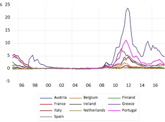
FIGURE 1 - 10-years government bond yield spread for 10 EMU countries along the period 1995-2017
Source: Reutters
Figure 1 depicts the evolution of the 10-year euro area government bond yield spreads versus Germany from 1995 until 2017. As can be seen, preceding the introduction of the euro there were some differences between spreads, but following 1999 the spreads are starting to converge. This convergence can be explained by the exchange rate risk elimination and also due to the rules of the Stability and Growth Pact that were perceived by the markets as trustworthy. Nevertheless, in the 2009, with the outbreak of the financial crisis, some of the economies experienced a large increase in their spreads versus Germany.
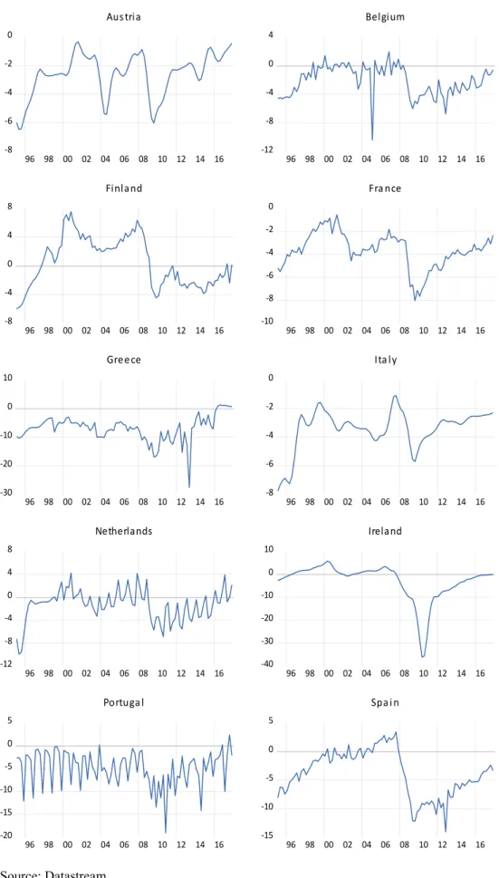
Figure 2 and 3 display the deterioration of the fiscal positions of the sample countries with the outburst of the sovereign debt crisis in early 2009. The fiscal deterioration means lower tax revenues and fiscal cost that government faces of having to support the financial
11
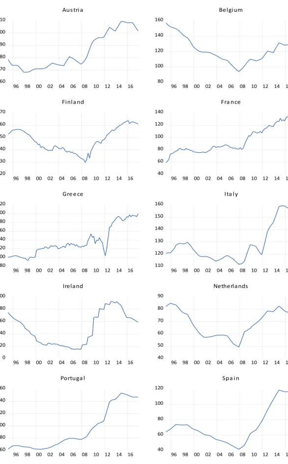
sector. As can be observed on the Figure 3, in all the sample countries, the expected debt as a percentage to GDP started to decrease only beginning in the 2016.
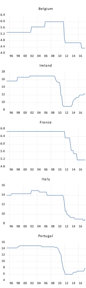
Finally, Figure 4 shows the evolution of the credit ratings of the sample countries for the study period. The data that was used comes from the tree main rating agencies, Standard and Poor´s, Moody´s and Fitch. Following the existing literature on ratings (see Afonso et al., 2012) the sovereign credit rating scores are transformed into the linear scale presented in Table A2 in the Appendix. For the periphery countries (Portugal, Spain, Ireland, Greece and Italy), after the significant deterioration of fiscal position the downgrade of the ratings was followinghad been undertaken by credit rating agencies.
12
FIGURE 3: Expected budget balance as percentage of GDP
-8 -6 -4 -2 0 96 98 00 02 04 06 08 10 12 14 16 Aus tria -12 -8 -4 0 4 96 98 00 02 04 06 08 10 12 14 16 Belgium -8 -4 0 4 8 96 98 00 02 04 06 08 10 12 14 16 Finla nd -10 -8 -6 -4 -2 0 96 98 00 02 04 06 08 10 12 14 16 Fra nce -30 -20 -10 0 10 96 98 00 02 04 06 08 10 12 14 16 Gre e ce -8 -6 -4 -2 0 96 98 00 02 04 06 08 10 12 14 16 Ita ly -12 -8 -4 0 4 8 96 98 00 02 04 06 08 10 12 14 16 Netherlands -40 -30 -20 -10 0 10 96 98 00 02 04 06 08 10 12 14 16 Ireland -20 -15 -10 -5 0 5 96 98 00 02 04 06 08 10 12 14 16 Portuga l -15 -10 -5 0 5 96 98 00 02 04 06 08 10 12 14 16 Spa i n Source: Datastream
13
FIGURE 4: Expected debt as percentage of GDP
60 70 80 90 100 110 96 98 00 02 04 06 08 10 12 14 16 Aus tri a 80 100 120 140 160 96 98 00 02 04 06 08 10 12 14 16 Belgium 20 30 40 50 60 70 96 98 00 02 04 06 08 10 12 14 16 Fi nla nd 40 60 80 100 120 140 96 98 00 02 04 06 08 10 12 14 16 Fra nce 80 100 120 140 160 180 200 220 96 98 00 02 04 06 08 10 12 14 16 Gre e ce 110 120 130 140 150 160 96 98 00 02 04 06 08 10 12 14 16 Ita l y 0 20 40 60 80 100 96 98 00 02 04 06 08 10 12 14 16 Ireland 40 50 60 70 80 90 96 98 00 02 04 06 08 10 12 14 16 Netherlands 60 80 100 120 140 160 96 98 00 02 04 06 08 10 12 14 16 Portuga l 40 60 80 100 120 96 98 00 02 04 06 08 10 12 14 16 Spa i n Source: Eurostat
14
FIGURE 5: Average credit ratings
14.0 14.4 14.8 15.2 15.6 16.0 16.4 96 98 00 02 04 06 08 10 12 14 16 Belgium 15.8 16.0 16.2 16.4 16.6 16.8 17.0 17.2 96 98 00 02 04 06 08 10 12 14 16 Aus tri a 8 10 12 14 16 18 96 98 00 02 04 06 08 10 12 14 16 Ireland 14.8 15.2 15.6 16.0 16.4 16.8 17.2 96 98 00 02 04 06 08 10 12 14 16 Finla nd 14.8 15.2 15.6 16.0 16.4 16.8 96 98 00 02 04 06 08 10 12 14 16 Fra nce 0 4 8 12 16 96 98 00 02 04 06 08 10 12 14 16 Gre e ce 8 10 12 14 16 96 98 00 02 04 06 08 10 12 14 16 Ita l y 16.6 16.7 16.8 16.9 17.0 17.1 96 98 00 02 04 06 08 10 12 14 16 Netherlands 4 6 8 10 12 14 16 96 98 00 02 04 06 08 10 12 14 16 Portuga l 8 10 12 14 16 18 96 98 00 02 04 06 08 10 12 14 16 Spa i n
15
3.3 Measuring core-periphery effect
While there is a difference between the determinants of government bond yield spreads for the pre- and post-crisis period, there is also a difference of the spread determinants between core and periphery group countries. As the core group countries are considered: Austria, Belgium, France, Finland and the Netherlands. Referring to the periphery group countries, those are Greece, Italy, Ireland, Portugal and Spain.
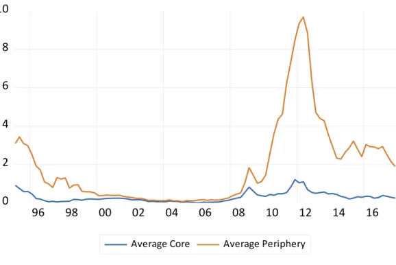
FIGURE 6: 10-years government bond yield speeds core-periphery groups
0 2 4 6 8 10 96 98 00 02 04 06 08 10 12 14 16
Average Core Average Periphery
Source: Reutters
Following the onset of the global financial crisis, as per Figure 6, the spreads of all countries that are analyzed in this study started to increase. The government bond yield spreads of the core group have been relatively stable, albeit at superior levels compared to the pre-crisis period. Meanwhile, the spreads of the periphery group, in the aftermath of the Lehman Brothers crisis, have been on an ascending path.
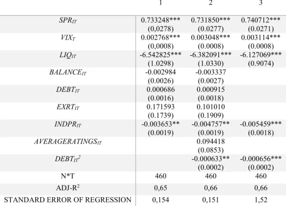
At the Table I are the results of the estimation of the equation (1) and (2) only for the core countries. All the variables have theoretically expected signs, except the average credit ratings. In first specification (equation (1)), can be noted that from all variables only three are significant for the model: international risk, market liquidity and industrial production. In more detailed equation (2), with average ratings and expected debt to GDP
16
in the second power, the significance of the variables from the first specification, remains the same, adding the nonlinear effect of the expected fiscal performance to the determinants of the spreads. In both specifications, fiscal performance and credit risk are not significant, so it can be concluded that for the core group countries these factors are not priced.
TABLEI:MODELING BOND YIELD SPREADS FOR CORE GROUP,2SLS
1 2 3 SPRIT 0.733248*** (0,0278) 0.731850*** (0.0277) 0.740712*** (0.0271) VIXT 0.002768*** (0,0008) 0.003048*** (0.0008) 0.003114*** (0.0008) LIQIT -6.542825*** (1.0298) -6.382091*** (1.0330) -6.127069*** (0.9074) BALANCEIT -0.002984 (0.0026) -0.003337 (0.0027) DEBTIT 0.000686 (0.0016) 0.000915 (0.0018) EXRTIT 0.171593 (0.1739) 0.101010 (0.1909) INDPRIT -0.003653** (0.0019) -0.004757** (0.0019) -0.005459*** (0.0018) AVERAGERATINGSIT 0.094418 (0.0853) DEBTIT2 -0.000633** (0.0002) -0.000656*** (0.0002) N*T 460 460 460 ADJ-R2 0,65 0,66 0,66
STANDARD ERROR OF REGRESSION 0,154 0,151 1,52
Note: The regression model is estimated over the time period 1995.Q1-20017.Q4 (T=92). The panel members include: Austria, Belgium, Finland, France, Netherlands, (N=5). Two Stage Least Squares (2SLS) fixed effect panel estimated, which account for endogeneity, are reported. The instruments used in the 2SLS estimations are the second lag of the dependent variable and the first three lagged values of the independent variables. Column 1 reports the results of the equation (1), the baseline model, while Column 2 presents the results of the equation (2), from the fully specified model. Column 3 presents only statistically significant variables from the equation (2). Standard errors in brackets. The asterisks ***, ** indicate significance at the 1% and, 5% level respectively.
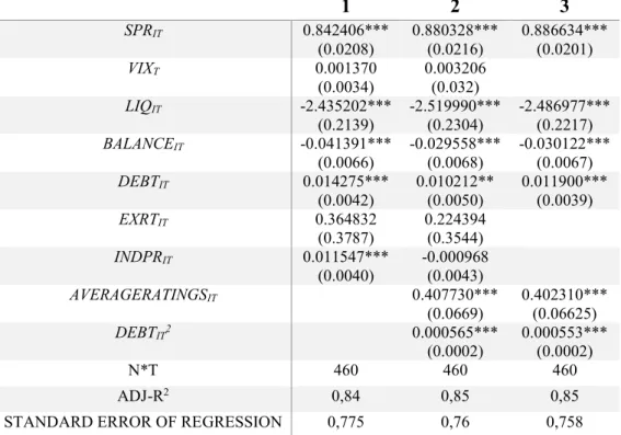
Next, the determinants of the government bond yield spreads for the group of periphery countries will be analyzed. In Table II are presented the outputs of both equations. The results of the equation (1) show that not all variables have economically expected signs. The industrial production is significant but has a positive sign. As can be seen, both indicators of fiscal stance are significant for the periphery group countries. The liquidity is also priced by the markets in this group.
17
Moving to the equation (2), the variables that were significant in the previous analyzes are also significant in this specification. Now only added average credit ratings factor presents not economically expected sign being significant. While it is expected that when there is an improvement of the rating position, the spread will decrease the multiplier has the positive sign. It can concluded that there is a nonlinear effect of expected fiscal performance on the government bond yield spread.
TABLEII:MODELLING BOND YIELD SPREADS FOR PERIPHERY GROUP,2SLS
1 2 3 SPRIT 0.842406*** (0.0208) 0.880328*** (0.0216) 0.886634*** (0.0201) VIXT 0.001370 (0.0034) 0.003206 (0.032) LIQIT -2.435202*** (0.2139) -2.519990*** (0.2304) -2.486977*** (0.2217) BALANCEIT -0.041391*** (0.0066) -0.029558*** (0.0068) -0.030122*** (0.0067) DEBTIT 0.014275*** (0.0042) 0.010212** (0.0050) 0.011900*** (0.0039) EXRTIT 0.364832 (0.3787) 0.224394 (0.3544) INDPRIT 0.011547*** (0.0040) -0.000968 (0.0043) AVERAGERATINGSIT 0.407730*** (0.0669) 0.402310*** (0.06625) DEBTIT2 0.000565*** (0.0002) 0.000553*** (0.0002) N*T 460 460 460 ADJ-R2 0,84 0,85 0,85
STANDARD ERROR OF REGRESSION 0,775 0,76 0,758
Note: The regression model is estimated over the time period 1995.Q1-20017.Q4 (T=92). The panel members include: Greece, Italy, Ireland, Portugal, Spain, (N=5). Two Stage Least Squares (2SLS) fixed effect panel estimated, which account for endogeneity, are reported. The instruments used in the 2SLS estimations are the second lag of the dependent variable and the first three lagged values of the independent variables. Column 1 reports the results of the equation (1), the baseline model, while Column 2 presents the results of the equation (2), from the fully specified model. Column 3 presents only statistically significant variables from the equation (2). Standard errors in brackets. The asterisks ***, ** indicate significance at the 1% and 5% level respectively.
Comparing two groups, it can be observed that in both cases the liquidity is priced by the markets. The nonlinear effect of expected fiscal performance on government bond spreads exists in either of the groups. While in core group countries markets don´t look at the financial stance of the economy in the periphery group both of them are priced. For the periphery group there are more factors that are taken into account to determine the
18
spreads it can be because those countries are considered as more risky compared to the core group.
3.4 Panel estimation results
To begin the analyzes of the benchmark model (equation (1)) and then its extension (equation (2)) were estimated for the full sample period for all countries. The results are reported in Table III.
TABLE III:MODELLING BOND YIELD SPREADS,2SLS
1 2 3 SPRIT 0.819561*** (0.0176) 0.809712*** (0.0184) 0.82231*** (0.0170) VIXT 0.045183** (0.0.0211) -0.416368 (0.0202) 0.127105*** (0.0202) LIQIT -2.589270*** (0.2116) -0.001837 (0.2677) BALANCEIT -0.006592** (0.0027) 0.016627*** (0.0019) DEBTIT 0.002966* (0.0016) 0.384670*** (0.0036) 0.017936*** (0.0035) EXRTIT 0.047816 (0.1689) 0.129925*** (0.1531) 0.332079** (0.1508) INDPRIT -0.001779 (0.0020) -0.003541** (0.0018) -0.003289* (0.0018) AVERAGERATINGSIT -0.451826*** (0.0551) -0.445376*** (0.0551) DEBTIT2 0.001110*** (0.0001) 0.000994*** (0.0001) N*T 920 920 920 ADJ-R2 0,79 0,79 0,79
STANDARD ERROR OF REGRESSION 0,522 0,606 0,611
Note: The regression model is estimated over the time period 1995.Q1-20017.Q4 (T=92). The panel members include: Austria, Belgium, Finland, France, Greece, Ireland, Italy, Netherlands, Portugal and Spain (N=10). Two Stage Least Squares (2SLS) fixed effect panel estimated, which account for endogeneity, are reported. The instruments used in the 2SLS estimations are the second lag of the dependent variable and the first two lagged values of the independent variables. Column 1 reports the results of the equation (1), the base line model, while Column 2 presents the results of the equation (2), from the fully specified model. Column 3 presents only statistically significant variables from equation (2). Standard errors in brackets. The asterisks ***, **,* indicate significance at the 1%, 5%, 10% level respectively.
The coefficients that were obtained, present all the theoretically expected signs defined in the previous section. In both specifications, spreads appear to be highly persistent. Regarding the significance of the variables, the liquidity is significant in the baseline model but then it is insignificant in the augmented model of equation (2). As for the expected fiscal fundamentals, they both appear to be significant in both specifications.
19
The squared debt is significant; therefore, there is a nonlinear effect of expected fiscal performance on government spreads.
TABLE IV:MODELLING BOND YIELD SPREADS WITH SLOPE-DUMMIES,2SLS
Note: The regression model is estimated over the time period 1995.Q1-20017.Q4 (T=92). The panel members include: Austria, Belgium, Finland, France, Greece, Ireland, Italy, Netherlands, Portugal and
1 2 3 SPRIT 0.832579*** (0.0189) 0.861792*** (0.0195) 0.852227*** (0.0169) VIXT -0.003937*** (0.0013) -0.003656*** (0.0013) -0.002684** (0.0011) VIXT *D1999.Q1 0.001318 (0.0015) 0.001764 (0.0015) VIXT *D2009.Q2 0.006755*** (0.0012) 0.006809*** (0.0012) 0.006693*** (0.0008) LIQIT 0.469154 (0.3823) 0.464356 (0.3940) LIQIT *D1999.Q1 -2.547036 (2.0834) -2.475530 (2.0795) LIQIT *D2009.Q2 -2.677692*** (0.3651) -2.570140*** (0.3777) -2.254807*** (0.2118) BALANCEIT -0.006290*** (0.0022) -0.005501*** (0.0022) -0.005062** (0.0021) BALANCEIT *D1999.Q1 -0.000547 (0.0037) -0.000223 (0.0036) BALANCEIT *D2009.Q2 -0.032600*** (0.0058) -0.030396*** (0.0058) -0.027765*** (0.0057) DEBTIT -0.024567*** (0.0035) -0.021571*** (0.0035) -0.018823*** (0.0031) DEBTIT *D1999.Q1 0.022370*** (0.0044) 0.018915*** (0.0044) 0.015213*** (0.0041) DEBTIT *D2009.Q2 0.022568*** (0.0044) 0.025509*** (0.0043) 0.021576*** (0.0039) EXRTIT 0.712844** (0.3015) 0.353187 (0.3062) EXRTIT *D1999.Q1 -1.230366** (0.4916) -0.870774* (0.4779) -0.724097** (0.3313) EXRTIT *D2009.Q2 -2.842641*** (0.7171) -2.031196*** (0.7286) -1.439392*** (0.5451) INDPRIT 0.003905 (0.0027) 0.002614 (0.0026) INDPRIT *D1999.Q1 -0.010488*** (0.0039) -0.009990*** (0.0039) -0.008676*** (0.0035) INDPRIT *D2009.Q2 0.001416 (0.0035) 0.004586 (0.0038) AVERAGERATINGSIT -0.155345 (0.2141) AVERAGERATINGSIT *D1999.Q1 0.161823 (0.2898) AVERAGERATINGSIT *D2009.Q2 0.440257** (0.2206) 0.319205*** (0.0572) N*T 920 920 920 ADJ-R2 0,82 0,83 0,83
20
Spain (N=10). The slope-dummy variables included to differentiate between 3 periods: D1999.Q1 and D2009.Q2.Two Stage Least Squares (2SLS) fixed effect panel estimated, which account for endogeneity, are reported. The instruments used in the 2SLS estimations are the second lag of the dependent variable and the first two lagged values of the independent variables. Column 1 reports the results of the equation (1), the base line model, while Column 2 presents the results of the equation (2), from the fully specified model. Column 3 presents only statistically significant variables from equation (2). Standard errors in brackets. The asterisks ***, **,* indicate significance at the 1%, 5%, 10% level respectively.
The proxy for the economic growth and the credit risk, both versus Germany, are significant in the second specification while international risk factor appears to be insignificant. As per this estimation, average credit ratings are also priced by the markets. To examine how the determinant of spreads change in the different periods of time the model is now expanded to analyze the results for the periods before and after sovereign crisis. To that end, the estimation of the equations is repeated accounting for slope-dummies, differentiating between three periods, namely, preceding the introduction of the euro (1995.Q1 – 1998.Q4), the period before the sovereign credit crisis (1999.Q1 – 2009.Q1) and finally the period after the sovereign credit crisis (2009.Q2 – 2017.Q4). Table IV reports the 2SLS estimation results.
Column (1) presents the results from the baseline model described by equation (1), including the time slope-dummies. Comparing to the previous outcome in this specification spread´s persistence is even higher. During the pre-crisis period, it can be seen that not so many variables were significant. As per results the credit risk factor, expected debt to GDP and the industrial production are main determinants of the spreads.
Regarding the period after first quarter of 2009, overall the liquidity risk, both determinants of fiscal stance, credit risk, economic growth rate and international risk are considered as the determinants of the government bond yield spreads. These results go in line with several previous studies.
Column (2) adds into the empirical specification the average credit ratings. In efficient markets and as long as the credit ratings are determinant by the publicly available information they should not be statistically significant determinants of spreads. The credit ratios are measured by a simple average rating scores provided by each of the three main rating agencies, namely Standard and Poor´s, Moody´s and Fitch. This method is used based on the study made by Afonso et al. (2012).
Table IV shows that credit rating are not significant prior the sovereign crisis, but they are significant after it with a positive sign. The inclusion of the credit ratings results in
21
small improvement of the explanatory power of the model. Regarding the other variables, we can see that the variables that were considered by the markets in the previous equation remain significant in this specification.
Finally, column (3) presents the results from a parsimonious specification obtained by moving from the general specification presented in column (2) towards a more specific model including only statistically significant variables. Based on the finding of this study, it can be concluded that in the period before the financial crisis the government bond yield spreads were mostly determined by the expected debt to GDP, the credit risk factor and economic growth.
With the eruption of the financial crisis, the analysis suggests that markets have started to take into consideration more fundamentals to determine the price of government bond yield spreads. International risk and the liquidity risk were two indicators that started to have a meaningful influence on spreads after 2009. Fiscal determinants, credit risk were also significant for this model. The average credit ratings while is significant in spread determination, after 2009 have unexpected relationship, presenting a positive sign. Overall, with the inclusion of the structural breaks, the model offers the superior information regarding the determinants of sovereign bond spreads in the euro area, especially for the period after 2009.
22 4.CONCLUSION
In this study were estimated the determinants of the government bond yields spreads in the euro area. The panel data of ten euro area countries was employed (Austria, Belgium, Finland, France, Greece, Ireland, Italy, Netherlands, Portugal and Spain) using quarterly data from 1995 to 2017. We investigated extended set of potential spreads’ determinants such as fiscal fundamentals, international risk, credit risk, liquidity conditions and credit ratings. After assessment of the benchmark model, the augmented equation was studied accounting for the structural breaks with two slope dummies differentiating between three periods, namely preceding the introduction of the euro (1995.Q1 – 1998.Q4), the period before the sovereign credit crisis (1999.Q1 – 2009.Q1) and finally the period after the sovereign credit crisis (2009.Q2 – 2017.Q4).
Based on the finding of this study, it can be concluded that in the period before the financial crisis the government bond yield spreads were mostly determined by the expected debt to GDP, the credit risk factor and economic growth.
With the eruption of the financial crisis, the analysis suggests that markets have started to take into consideration more fundamentals to determine the price of government bond yield spreads. International risk and the liquidity risk were two indicators that started to have a meaningful influence on spreads after 2009. Fiscal determinants, credit risk were also significant for this model. The average credit ratings while is significant in spread determination, after 2009 have unexpected relationship, presenting a positive sign. Looking further ahead, greater market discrimination across countries may provide higher incentives for governments to attain and maintain sustainable public finances. Since even small changes in bond yields have a noticeable impact on government outlays, market discipline may act as an important deterrent against deteriorating public finances.
23 REFERENCES
Acharya, V.V., Drechsler, I. and Schnabl, P. (2011). “A Pyrrhic victory? – Bank bailouts and sovereign credit risk”. NBER Working Paper 17136.
Afonso, A., Arghyrou, M., Gadea, M., Kontonikas, A. (2018). "Whatever it takes” to resolve the European sovereign debt crisis? Bond pricing regime switches and monetary policy effects". Journal of International Money and Finance, Volume 86, 1-30.
Afonso, A., Arghyrou, M., Kontonikas, A. (2015). "The determinants of sovereign bond yield spreads in the EMU". European Central Bank. Working Paper, 1781.
Afonso, A., Furceri, D. and Gomes, P. (2012). “Sovereign credit ratings and financial markets linkages: application to European data”. Jornal of International Money and Finance, 31, 606-638.
Afonso, A. and Rault, P. (2010). "Short and Long-run behavior of long-term sovereign bond yield". Applied Economics, Working Paper 19, 1-37.
Arghyrou, M.G. and Kontonikas, A. (2011). “The EMU sovereign-debt crisis: Fundamentals, expectations and contagion”. European Comission Economic Papers 436. Barbosa, L., Costa, S. (2010). "Determinants of sovereign bond yield spreads in the Euro Area in the context of the economic and financial crisis”. Banco de Portugal: Estudos e Documentos de Trabalho, 22, 1-44.
Barrios, S., Iversen, P., Lewandowska, M. and Setzer, R. (2009). "Determinants of intra-euro area government bond spreads during the financial crisis". European Comission, Economic Paper, 388.
Beber, A., Brandt, M. and Kavajecz, K. (2009). “Flight-Quality or Flight to-Liquidity? Evidence from the Euro-Area Bond Market” Review of Financial Studies, 22, 925-957.
Bernoth, K., von Hagen, J., Schuknecht, L. (2004). “Sovereign spreads: Global risk aversion, contagion or fundamentals?” IMF Working Paper 10/120.
Bernoth, K., Wolff, G. (2008). “Fool the markets? Creative accounting, fiscal transparency and sovereign risk premia”. Scottish Journal of Political Economy, 55, 465-487.
24
Codogno, L., Favero, C., Missale, A. (2003). “Yield spreads on EMU government bonds”. Economic Policy, 18, 211-235.
Favero, C. and Missale, A. (2011). “Sovereign Spreads in the Euro Area. Which Prospects for a Eurobond?” CEPR Discussion Paper Nº8637.
Favero, C., Pagano, M. and von Thadden, E.-L. (2010) "How Does Liquidity Act Government Bond Yields?” Journal of Financial and Quantitative Analysis, 45.
Gerlach, S., Schulz, A., Wolf, G. (2010). “Banking and sovereign risk in the euro area”. CERP Discussion Paper No.7833.
Gomez-Puig, M. (2006). "Size matters for liquidity: Evidence for EMU sovereign yield spreads". Economics Letters, 90, 156-162.
Hallerberg, M., Wolff, G.B. (2008). “Fiscal institutions, fiscal policy and sovereign risk premia in EMU”. Public Choice, 136, 379-396.
Haugh, D., Ollivaund, P., Turner, D. (2009). “What Drives Sovereign Risk Premiums? An Analysis of Recent Evidence from the Euro Area”, OECD Economics Department Working Papers, No. 718.
Hui, C.H., Chung, T.K. (2011). "Crash risk of the euro in the sovereign debt crisis of 2009–2010". Journal of Banking and Finance, 35, 2945-2955.
Jankowitsch, R., Mosenbacher, H., Pichler, S. (2002).” Measuring the Liquidity Impact on EMU Government Bond Prices”. European Journal of Finance, 12.
Manganelli, F. Wolswijk, G. (2007). “What drives spreads in the euro-area government bond market”. European Central Bank. Working Paper 745.
Pagano, M., von Thaden, E.L. (2004). "The European Bond Markets under EMU". Oxford Review of Economic Policy.
Schuknecht, L., von Hagen, J., Wolswijk, G. (2010). "Government bond risk premium in the bond market: EMU and Canada". European Journal of Political Economy", 25, 371-384.
25 APPENDICES
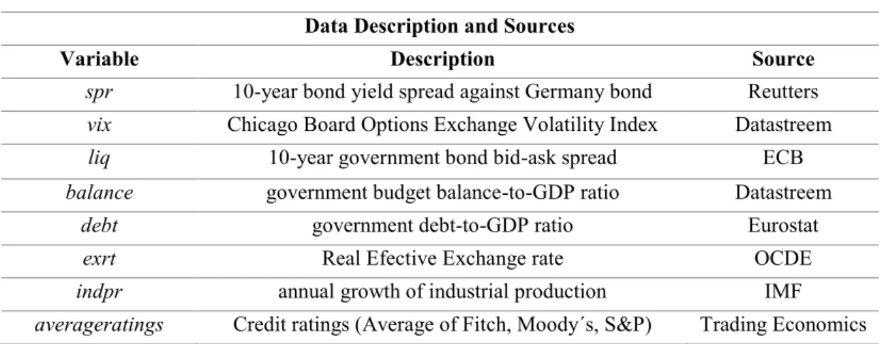
TABLEA1:DATA DEFINITION AND SOURCES
Data Description and Sources
Variable Description Source
spr 10-year bond yield spread against Germany bond Reutters vix Chicago Board Options Exchange Volatility Index Datastreem liq 10-year government bond bid-ask spread ECB balance government budget balance-to-GDP ratio Datastreem
debt government debt-to-GDP ratio Eurostat exrt Real Efective Exchange rate OCDE indpr annual growth of industrial production IMF averageratings Credit ratings (Average of Fitch, Moody´s, S&P) Trading Economics
TABLE A2:S&P,MOODY’S AND FITCH RATING SYSTEMS
Source: Afonso et al., 2012
Characterization of debt and issuer
Linear
transformation S&P Moody´s Fitch
Highest quality AAA Aaa AAA 17
AA+ Aa1 AA+ 16
AA Aa2 AA 15
AA- Aa3 AA- 14
A+ A1 A+ 13 A A2 A 12 A- A3 A- 11 BBB+ Baa1 BBB+ 10 BBB Baa2 BBB 9 BBB- Baa3 BBB- 8 Likely to fulfil obligations, BB+ Ba1 BB+ 7 BB Ba2 BB 6 ongoing uncertainty BB- Ba3 BB- 5 B+ B1 B+ 4 B B2 B 3 B- B3 B- 2 CCC+ Caa1 CCC+ CCC Caa2 CCC CCC- Caa3 CCC-Near default with possibility of recovery C SD C DDD D DD D Ratings 1 Very high credit
risk CC Ca CC Default Adequate payment capacity Sp ec ul ati ve gr ad e
High credit risk High quality Strong payment capacity In ve stme nt gr ad e