UNIVERSIDADE DE ÉVORA
DEPARTAMENTO DE ECONOMIA
DOCUMENTO DE TRABALHO Nº 2005/09
May
How to Classify a Government?
Can a Neural Network do it?
1st version: February 09, 2005
This version: April 25, 2005 António Caleiro *
Universidade de Évora, Departamento de Economia
* Paper given at the XII Jornadas de Classificação e Análise de Dados, Universidade dos Açores, Ponta Delgada (April 22, 2005).
I would like to thank Steffen Hörnig for an extremely useful suggestion. Obviously, the usual disclaimer applies.
UNIVERSIDADE DE ÉVORA DEPARTAMENTO DE ECONOMIA
Largo dos Colegiais, 2 – 7000-803 Évora – Portugal Tel.: +351 266 740 894 Fax: +351 266 742 494
Abstract:
An electoral cycle created by governments is a phenomenon that seems to characterise, at least in some particular occasions and/or circumstances, the democratic economies.
As it is generally accepted, the short-run electorally-induced fluctuations prejudice the long-run welfare. Since the very first studies on the matter, some authors offered suggestions as to what should be done against this electorally-induced instability. A good alternative to the obvious proposal to increase the electoral period length is to consider that voters abandon a passive and naive behaviour and, instead, are willing to learn about government’s intentions.
The electoral cycle literature has developed in two clearly distinct phases. The first one considered the existence of non-rational (naive) voters whereas the second one considered fully rational voters. It is our view that an intermediate approach is more appropriate, i.e. one that considers learning voters, which are boundedly rational. In this sense, one may consider neural networks as learning mechanisms used by voters to perform a classification of the incumbent in order to distinguish opportunistic (electorally motivated) from benevolent (non-electorally motivated) behaviour of the government. The paper explores precisely the problem of how to classify a government showing in which, if so, circumstances a neural network, namely a perceptron, can resolve that problem.
Keywords: Classification, Elections, Government, Neural Networks, Output Persistence, Perceptrons
1. Introduction and Motivation
An electoral cycle created by governments is a phenomenon that seems to characterise, at least in some particular occasions and/or circumstances, the democratic economies. As it is generally accepted, the short-run electorally-induced fluctuations prejudice the long-run welfare. Since the very first studies on the matter, some authors offered suggestions as to what should be done against this electorally-induced instability. For
some authors, ever since the seminal paper of NORDHAUS (1975), a good alternative to
the obvious proposal to increase the electoral period length is to consider that voters abandon a passive and naive behaviour and, instead, are willing to learn about government’s intentions.
The electoral cycle literature has developed in two clearly distinct phases. The first one, which took place in the mid-1970s, considered the existence of non-rational (naive) voters. In accordance with the rational expectations revolution, in the late 1980s the second phase of models considered fully rational voters. It is our view that an intermediate approach is more appropriate, i.e. one that considers learning voters, which are boundedly rational. In this sense, one may consider neural networks as learning mechanisms used by voters to perform a classification of the incumbent in order to distinguish opportunistic (electorally motivated) from benevolent (non-electorally motivated) behaviour of the government. The main objective of this paper consists precisely on studying the problem of how to classify a government showing in which, if so, circumstances a neural network, namely a perceptron, can resolve that problem. To achieve this objective we will consider a quite recent version of a stylised model of economic policy, i.e. a version based on an aggregate supply curve embodying output
persistence. See GÄRTNER (1996,1997,1999,2000).
The rest of the paper is structured as follows. Section 2 offers the analysis of the bounded rationality approach as a motivation for the use of neural networks as learning devices. Section 3 then presents the characteristics of the particular neural network, i.e. the perceptron, which will be used to perform the classification of the government task. Section 4 explores the problem of how to classify a government showing in which, if so, circumstances the perceptron can resolve that problem. Section 5 concludes.
2. The Bounded Rationality Approach
In the spirit of the bounded rationality research program, which is really to put the economist and the agents in his model on an equal behavioral footing, we expect that, in searching these literatures for ways to model our agents, we shall find ways to improve ourselves. in
SARGENT (1993), pg. 33.
Generally speaking, learning models have been developed as a reasonable alternative to the unrealistic informational assumption of rational expectations models. Moreover, through learning models it is possible to study the dynamics of adjustment between equilibria which, in most rational expectations models, is ignored. In fact, rational expectations hypotheses are, in some sense and with some exceptions, a limiting property of a dynamic system which evolves from one equilibrium to another, this being possible because it is assumed that agents know the true model of the economy and use it to form their expectations which, in turn, implies that agents are also able to solve the model.
Interestingly, learning models also deal with another difficulty of rational expectations models, namely the existence of multiple equilibria. It is well known that for linear models, where only expectations of current variables are considered, the rational expectations equilibrium is unique. Conversely, when expectations about the future endogenous variables are required, multiple rational expectations equilibria can occur. Moreover, this is also a common feature of stochastic control/decision problems. In this case, the lack of equilibrium uniqueness arises from an imperfectly specified intertemporal decision problem under uncertainty. The analysis of learning processes can, in fact, provide a way of selecting the ‘reasonable’ equilibrium or sub-set of equilibria. On the one hand, if the learning mechanism is chosen optimally, then a
desirable rational equilibrium is selected from the set of the rational expectations
equilibria; see MARCET and SARGENT (1988,1989a,1989b). On the other hand, if the learning mechanism is viewed under an adaptive approach, in particular in
expectational stability models, it can also act as a selection criterion in multiple
equilibria models involving bubbles and sunspots; see EVANS (1986), EVANS and GUESNERIE (1993), EVANS and HONKAPOHJA (1994,1995). To sum up, learning mechanisms, whether optimally or adaptively chosen, ‘select’ the particular steady state
as, in some sense, terminal conditions do.
Through this last point, one can already anticipate the usual distinction between learning mechanisms. Although a number of different studies modelling learning have been presented, two main classes of models can be distinguished: rational learning and boundedly rational learning models.3 In rational learning models, it is assumed that agents know the true structural form of the model generating the economy, but not some of the parameters of that model. In boundedly rational learning models, it is assumed that agents, while learning is taking place, use a ‘reasonable’ rule, for instance, by considering the reduced form of the model.
Rational learning, which some authors identify with Bayesian learning, thus assumes that the model structure is known by the agents while the learning process is taking place. Given the difficulties that arise in modelling this kind of learning, the bounded rationality approach has the appealing advantage of being (at least) more tractable. Moreover, the assumption that agents use a misspecified model during the learning process makes the bounded rationality approach less controversial.
Obviously, the use of a misspecified model during learning has its consequences on the formation of expectations. In fact, under the bounded rationality approach, agents are modelled as using an ‘incorrect’ rule, derived from backward-looking reduced form equations, to generate expectations while they are learning about the true structural form.
In the bounded rationality approach, various notions of expectational stability and of
econometric learning procedures have been the main formulations. Interestingly, the
distinction between these two main procedures has to do with the ‘notion’ of time where learning takes place. While the expectational stability principle assumes that learning takes place in ‘notional’, ‘virtual’ or meta-time, econometric learning procedures
3
WESTAWAY (1992) prefers to distinguish closed-loop learning, where agents learn about the parameters of the decision rule, from open-loop learning, where agents form an expectation of the path for a particular variable which they sequentially update. As is pointed out, closed-loop learning will be virtually identical to the parameter updating scheme using Kalman filtering.
5
If agents never discount past information, then Kalman filtering can be seen as a rolling least-squares regression with an increasing sample. On the contrary, if past information becomes less important, then a ‘forgetting factor’ can be included which gives a rolling window, or more precisely a form of weighted
assume real-time learning.
The expectational stability approach considers the influence of – and thus the distinction between – perceived laws on actual laws of motion of the economic system. The actual law of motion results from the substitution of the perceived law of motion in the structural equations of the true model. It is then possible to obtain a mapping L
( )
θ
from the perceived to the actual law of motion, where θ denotes the set of parameters. Rational expectations solutionsθ
are then the fixed points of L( )
θ . Finally, a given rational expectations solutionθ
is said to be expectationally-stable if the differential equation:( )
θ
θ
τ
θ
= − L d dis locally asymptotically stable at
θ
, where τ denotes meta-time.In adaptive real-time learning, agents are assumed to use an econometric procedure for estimating the perceived law of motion. Least-squares learning is widely used in this formulation in spite of its apparent drawbacks; see SALMON (1995) for a criticism of
this issue. A more sophisticated application of these econometric procedures is the consideration of the Kalman filter which, as is well known, nests least squares learning and recursive least squares.5
Given the above discussion we can question, as WESTAWAY (1992) clearly and
naturally points out:
“How do policymakers react to the fact that the private sector is learning?” Paradoxically, this pertinent question has been almost ignored. In fact, the analysis of the implications of learning mechanisms in policy-making is far from being complete.
Some exceptions are BARRELL et al. (1992), BAŞAR and SALMON (1990a,1990b),
least squares.
7
A more formal definition would consider a neural network <P,p> to be a directed graph over the set
CRIPPS (1991), EVANS and HONKAPOHJA (1994), FUHRER and HOOKER (1993), MARIMON and SUNDER (1993,1994), SALMON (1995) and WESTAWAY (1992). SALMON
(1995) is, to the best of my knowledge, one of the very few references where an innovative bounded rationality approach such as neural networks learning has been
applied in a policy-making problem. We propose to use this approach within a political business cycles context. That being said, we will consider that bounded rationality voters have to classify economic policies and outcomes as coming from opportunistic or
from benevolent government behaviour.
3. The Neural Networks Methodology
Given the characteristics of neural networks it, thus, seems appropriate to consider that
the above mentioned classification task can be performed under this formulation of bounded rationality agents. Given that (artificial) neural networks are simulations of how biological neurons are supposed to work, the structure of human brains, where
processing units, the so-called neurons, are connected by sinapses, is approximated by
these (artificial) neural networks. As such, the interconnected network of processing
units describes a model which maps a set of given inputs to an associated set of outputs
values.7 As the number of inputs does not have to be equal to the number of outputs, a
neural network can, alternatively, be described as mapping one set of variables onto another set of a possibly different size.
The knowledge of the values for the input and output variables constitutes, then, the major part of the information needed to implement a neural network. Despite the minimal information requirement, this constitutes no motive for questioning the results obtained; see SALMON (1995). In fact, this characteristic makes neural networks particularly appropriate for cases where the structure connecting inputs to outputs is
unknown.8 In this sense, neural networks can be classified as ‘non-structural’
procedural models. Furthermore, they are in good agreement with a typical
characteristic of bounded rationality: the adaptive behaviour. Indeed, the adaptation to
8
Take, for instance, WALL (1993) which pretends to bridge the gap between substantive rationality and
procedural rationality. The fact that it is considered that the exact form of the objective function is
unknown is what makes this bounded rationality model a good example of a possible application of neural networks.
the environment as a crucial characteristic of a neural network makes it distinct from
many (standard) models of learning.9
Neural networks are used mainly to learn in two types of tasks; see SWINGLER (1996):
1. Continuous numeric functions – When the task is to approximate some
continuous function, as in the case of a signal extraction.
2. Classification – When the input is a description of an object to be recognised and
the output is an identification of the class to which the object belongs. The most
common kind of neural network for classification purposes is the so-called
perceptron.10 In what follows it will be shown how perceptrons would classify policies and outcomes as ‘electoralist’ or not, using a recent stylised model of economic policy.
Let us then clarify the modus operandi of neural networks by a simple formalisation as
follows.11 Given an input vector x, the neural network determines a particular
parameterisation, say β, which, in conjunction with a function g – also possibly
determined by the neural network – leads to the output vector y=g
( )
x,β ‘closest’ to some target y*. In other words, the output units y( )
k ,(
k =1,...,t)
, process, using a function g, the inputs x( )
i,(
i=1,...,r)
, previously amplified or attenuated by the connection strengths β( )
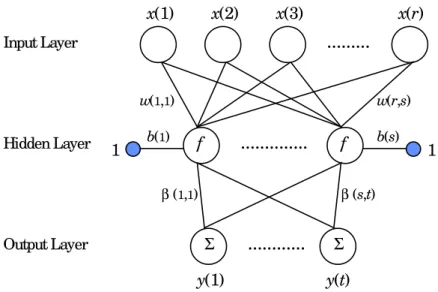
i,k .12The simplest neural network structure described above is usually relaxed to obtain flexibility by considering a layer of, so-called, hidden units. In this case, the transformation of inputs into outputs includes an intermediate processing task performed by the hidden units. Each hidden unit, then, produces, by the consideration of
9
In particular, neural networks relax the constant linear reduced form assumption of least squares
learning by considering a time varying possibly non-linear stochastic approximation of that reduced form.
10
For a clear explanation of the link between perceptrons and the statistical discriminant analysis see CHO
and SARGENT (1996).
11
To all of those whose scepticism only disappears with a sound mathematical presentation see ELLACOTT and BOSE (1996). More advanced references include WHITE (1989).
12
Implicitly assumed is a feedforward model where signals flow only from x(i) to y(k). Nevertheless, it is also possible to consider feedback effects.
an activation or transfer function f(.), an intermediate output s(j), (j = 1,…,s), which is finally sent to the output layer.13 This situation can be illustrated as follows.
x(2) x(3) x(r)
...
...
x(1) w(1,1) w(r,s) b(1) b(s) 1 1 Input Layer Hidden Layer...
Output Layer y(1) y(t) β (1,1) β (s,t) Σ Σ f fFigure 1 – The neural network structure
Mathematically the network then computes:
1. The input(s) to the hidden layer, h(j), as a weighted sum
( ) ( )
( ) ( )
, 1,..., ; 1 s j i x j i w j b j h r i = + =∑
=2. The output(s) of the hidden layer, which are the input(s) to the output layer, are
subject to an output activation
( )
j f( )
h( )
j ,s =
where f is the so-called activation function. 3. The output(s) of the output layer14
( )
( ) ( )
, 1,..., . 1 t k j s k j k y s j = =∑
=β
Plainly the two crucial elements of a neural network are the parameter set θ =
(
w,β)
and the activation/transfer function f(.). The transfer function usually has the role of13
It is also (and generally) possible to consider a bias node ‘shifting' the weighted sum of inputs by some factor b (j). See Figure 1.
14
It is possible to consider an activation function and/or a bias before the determination of the ‘final’ outputs.
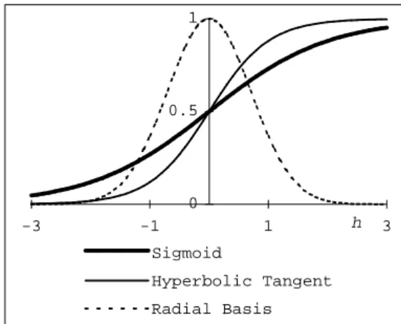
normalising a node’s output signal strength between 0 and 1.15 The most used are the
tanh or some sigmoid function f
( )
h =(
1+exp( )
−h)
−1 and a gaussian function orsome radial basis function. The differences between these functions are made clear
by considering the following figure.
0 0.5 1 -3 -1 1 h 3 Sigmoid Hyperbolic Tangent Radial Basis
Figure 2 – Some squashing functions
As is clear, the sigmoid and the tanh functions are similar. Moreover, while the radial
basis function amplifies in-between values, the sigmoid and tanh functions attenuate
or amplify extreme values. Clearly, their differences in practice result also from the specific parameterisation θ.
As usual, once the parameters have been set, say θˆ , the neural network is able to predict outputs yˆ =g
( )
x,θ
ˆ for input values x which were not included in the training data.3.1. The learning process
As pointed out in WHITE (1989), the output vector y=g
( )
x,θ can be viewed as generating a family of approximations (as θ ranges over the set Θ, say) for theunknown relation between inputs x and their corresponding outputs y. The best
approximation can be determined by a recursive learning procedure known as back-propagation. The learning process – training – is then an iterative procedure of processing inputs through the neural network, determining the errors and
15
propagating the errors through the network to adjust the parameters in order to minimise the error between the predicted and observed outputs. This method of learning is referred to as gradient descent as it involves an attempt to find the lowest point in the error space by a process of gradual descent along the error surface.16
In our case, a single-layer network known as perceptron will be used to perform the classification task or, in other words, will be used to determine the vector of weights and bias specifying a line on the space output-inflation such that two sub-sets of points – obviously the opportunistic and benevolent ones – are defined. At this stage, a short explanation about how the neural network will determine the above-mentioned vector seems appropriate.
In the particular case under study, the learning process conducing to the above-mentioned vector of weights and bias can thus be described as follows:
1. Initial weights, w, and bias, b, are generated in an interval with enough range;17
2. Given some target vector y*, with binary values associated with the two
considered categories of governments, the error, e, is computed as the difference between y* and the perceptron output y.
i) If there is no error in the classification, that is e = 0, then ∆w=∆b=0; ii) If some pair of economic policies/states is classified as belonging to category
1, say benevolent, and should have been classified as belonging to category 0, say opportunistic, then e = -1. Therefore, in order to increase the chance that the input vector x will be classified correctly, the weight vector w is ‘put farther away’ from x by subtracting x from it; this meaning that
T
x w=−
∆ ;
iii) If some pair of economic policies/states is classified as belonging to category 0 and should have been classified as belonging to category 1 , then e = 1. Therefore, in order to increase the chance that the input vector x will be
16
Two factors are used to control the training algorithm’s adjustment of the parameters: the momentum
factor and the learning rate coefficient. The momentum term, which is quite useful to avoid local minima,
causes the present parameter changes to be affected by the size of the previous changes. The learning rate dictates the proportion of each error which is used to update parameters during learning.
17
Note that a hard limit transfer function will be used and this gives y = 1 when wx + b > 0 and y = 1 when wx + b ≤ 0
classified correctly, the weight vector w is ‘put closer’ to x by adding x to it; this meaning that ∆w=xT.
To sum up, the perceptron learning rule will be based upon the following updating rules:
(
y y)
xT exT, w= − = ∆ ∗ (1) and(
y y)
T e. b= − = ∆ ∗ 1 (2)Using (1) and (2) repeatedly – the so-called training process – the perceptron will eventually find a vector of weights and bias, such that all the pairs of inflation and output are classified correctly. Indeed, it is well known that, if those pairs are linearly separable, the perceptron will always be able to perform the classification by determining a linear decision boundary.
4. The Classification of the Government
In the electoral business cycle literature, one of the most crucial conclusions is that the short-run electorally-induced fluctuations prejudice the long-run welfare. In fact, because the electoral results depend on voters’ evaluation, we can consider that if electoral business cycles do exist it is because voters, through ignorance or for some other reason, allow them to exist. This point introduces a well-known problem of
electorally-induced behaviour punishment and its related problem of monitoring. In reality, voters often cannot truly judge/classify if an observed state/policy is the result of a self-interested/opportunistic government or, on the contrary, results as a
social-planner/benevolent outcome, simply because voters do not know the structure, the model or the transmission mechanism connecting policy values to state values. Moreover, a constant monitoring of government behaviour seems not to be considered a crucial practice by the electorate.
Even so, voters do ‘anticipate’ the possible economic damage resulting from such
policies and outcomes as potentially being the result of an ‘electoralist’ strategy. This is done in order not to be ‘fooled’ by the incumbent government or simply to punish the incumbent government in case of clear signals of electorally-induced policies. In other words, a classification is made, so that for a sufficiently small sub-set of policies classified as ‘electoralist’, voters usually do not take that as a serious motive for punishment, but others, regarded as serious deviations, are punished.18 In general, this classification task is made difficult by ignorance of the structural form of the model transforming policies in outcomes and also simply because information gathering costs money and time.
4.1. The model
Recently some authors have assumed an extended version of the standard aggregate supply curve yt = y+
β
(
π
t −π
te)
, where yt denotes the level of output (measured in logarithms) that deviates from the natural level, y , whenever the inflation rate,π
t, deviates from its expected levelπ
te, by considering(
)
(
e)
t t t t y y y = 1−η +η −1+δ π −π , (3)where
η
measures the degree of output persistence. See GÄRTNER (1999) for an outputpersistence case and/or JONSSON (1997) for an unemployment persistence case.19
When normalizing the natural level of output such that y=0 the aggregate supply curve reduces to:
(
e)
t t t t y y =φ −1+α π −π , (4)where, following the hypothesis of adaptive expectations,
1 − = t e t γπ π , (5) 18
Note the difference between this approach and the one considered, for instance, in MINFORD (1995). Here, it is assumed that “voters penalise absolutely any evidence that monetary policy has responded to
anything other than news”, by ‘absolutely’ meaning that there is enough withdrawal of voters to ensure
electoral defeat.
19
As acknowledged in GÄRTNER (1999), only quite recently authors have started to pay due attention to
the consequences of considering that relevant macroeconomic variables, in reality, show some degree of persistence over time. In fact, a casual observation on reality shows that Europe has been facing a problem in what concerns unemployment which indeed reflects persistence. Given the close connection between unemployment and output, it should be possible to ‘translate’ our results in terms of output to results in terms of unemployment.
where 0≤
φ
≤1 and 0≤γ
≤1.As said before, a most common kind of neural network for classification purposes is the so-called perceptron. In order to perform the task of classifying the government, in what concerns its behaviour during the mandate, it is required the determination of the opportunistic and benevolent solutions. These solutions differ in accordance with the way time periods are discounted: whereas for society, therefore also for a benevolent government, future periods should be less important than present ones, this is not the case with an opportunistic government, as future moments, i.e. those closer to the election day, are more vital than present ones, in order to explore the decay in the memory of voters.
Having said that, concerning the government's objective function, we make the standard assumption that the incumbent faces a mandate divided into two periods, t =1,2, such that society’s welfare during the mandate, i.e. the benevolent government's objective function is given by:
2 1 U
U
U = +ρ , (6)
where
ρ
is the social rate of discount, whereas opportunistic government's objective function is :2 1 V
V
V =µ + , (7)
where
µ
is the degree of memory of the electorate. In (6) and (7) we also admit thatt t t
t V y
U = =−21π2+β . (8)
In these circumstances it is worth immediately noticing that, in general, excepting if 1
=
µρ
, the policies that maximise social welfare (6) are not the ones that maximise popularity (7). As it plausible to assume that bothρ
andµ
do not exceed 1, it isimmediately clear that only in the case of perfect memory, i.e.
µ
=1, and both periodsbeing equally important for society, i.e.
ρ
=1, an opportunistic government will behave exactly as a benevolent one. This fact allows for making it plausible to ask the question:how to classify a government?, whose answer is supposed to be given by a neural
network when separating optimal outcomes into two parts: the opportunistic and the benevolent ones. In other words, the opportunistic and benevolent solutions (policies
and outcomes) will constitute the necessary inputs for the neural network application. Given the classification task format, let us precisely define what will be called
opportunistic or ‘electoralist’ inputs, that is policies, and opportunistic outputs, that is
outcomes, to be compared with benevolent inputs and benevolent outputs.
Clearly, the opportunistic policy and outcomes will be, respectively, the values of inflation and output which result from the maximisation of (6) and (7) subject to (4) and (5). This immediately leads to the optimal policies:20
(
)
(
ρ
γ
φ
)
αβ
π
1B = 1− − , (9)αβ
π
B = 2 , (10) − − = µ φ γ αβ π1O 1 , (11)αβ
π
O = 2 . (12)Those policies lead to the optimal output levels:
(
)
(
)
(
0)
0 1 =φy +α αβ 1−ρ γ −φ −γπ yB , (13)(
)
(
)
(
)
(
φ α αβ ρ γ φ γπ)
α(
αβ γαβ(
ρ(
γ φ)
)
)
φ + − − − + − − − = 0 1 0 1 2 y yB , (14) − − − + = 0 0 1 1 µ γπ φ γ αβ α φy yO , (15) − − − + − − − + =µ
φ
γ
γαβ
αβ
α
γπ
µ
φ
γ
αβ
α
φ
φ
0 1 0 1 2 y yO . (16)Before proceeding with the classification task, it is relevant to note that there are, in fact, two possible patterns for the political business cycle: i) a typical one, where inflationary expansions take place immediately before the elections and ii) an atypical one, where the inflationary expansions take place immediately after the elections.21 Given that:
20
From this point onwards, the superscripts B and O identify an element as, respectively, concerning the benevolent and the opportunistic government.
21
This means that, in general, not possible to always use the observed pre-elections expansions as empirical evidence supporting the existence of an opportunistic behaviour of the government as, in fact, even some experienced scholars incorrectly do.
(
γ φ)
αβρ π πB − B = − 1 2 , µ φ γ αβ π πO− O = − 1 2 ,the typical pattern will be observed when
γ
>φ
and the atypical one whenγ
<φ
. Plainly, whenγ
=φ
there will be no cycle at all.Given the optimal solutions, (9) to (16), it is straightforward to verify that, because
(
γ φ)
µµρ αβ π π1 − 1 = − 1− O B , 2 − 2 =0 O B π π ,(
γ φ)
µµρ β α − − = − 2 1 1 1 O B y y ,(
)
µµρ φ γ β α − − − = − 2 21 1 1 O B y y ,the typical pattern will then be characterised by:
B B 1 2 π π > , π2O >π1O, O B 1 1 π π > , π2B =π2O and O B y y1 > 1 , y2B <y2O, whereas the atypical pattern will be characterised by:
B B 1 2 π π < , π2O <π1O, π1B <π1O, π2B =π2O and O B y y1 < 1 , O B y y2 < 2 .
Given that, in the previous mandate, no matter the kind of government,
αβ
π0 = , (17)
it is possible to further simplify the optimal output levels expressions, (13) to (16), to:
(
)
(
ρ γ φ γ)
β α φ + − − − = 0 2 1 1 y yB , (18)(
φ φργ ρφ φγ γ γ ρ)
β α φ 2 2 2 0 2 2 = y + −2 + − +1− + yB , (19) µγ γµ φ µ β α φ + + − − = 2 0 1 y yO , (20) − − − + + − − + = µφ γ γαβ αβ α µγ γµ φ µ β α φ φ 0 2 1 2 y yO . (21)4.2. The classification task
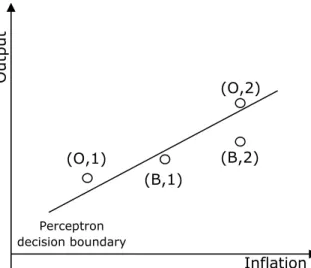
coordinates of four points in the
( )
y,π plane. This space is to be partioned, if possible, in two sub-spaces by a linear decision boundary – in that consists the classification task – by the neural network. See figure 3.O u tpu t Inflation (B,1) (B,2) (O,2) (O,1) Perceptron decision boundary
Figure 3 – The neural network classification
Figure 3 allows visualising the opportunistic and benevolent trajectories in the
inflation-output, (y,π), space, showing an example where the classification of the government is
possible to be achieved by that kind of neural network.
There are, therefore, four points located in the (y,π) space, two of each type, O and B.
This makes possible to draw two line segments connecting the two points of each kind. If these two line segments cross, it is impossible to obtain a decision boundary. This can be checked by a system of equations involving two convex combinations between these points defining the intersection between the straight line segments. They cannot be separated if the two parameters, λ1,λ2 in the convex combinations:
(
)
(
)
− + = − + O O O O B B B B y y y y 2 2 2 1 1 2 2 2 1 1 1 1 1 1π
λ
π
λ
π
λ
π
λ
, (22)are both between 0 and 1.
Given the optimal inflation rates, (9) to (12), and output levels, (18) to (21), the solutions for λ1,λ2 in (22) are:
(
)
(
1)
0 2(
1)
2 2 1 − + − − =γ
β
α
φ
φ
γ
φµ
β
α
λ
y , (23)(
)
(
1)
0 2(
1)
2 2 2 − + − − =γ
β
α
φ
φ
γ
φ
βρ
α
λ
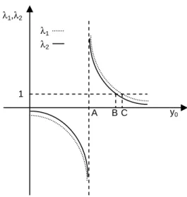
y . 22 (24)Plainly, in general, the possibility to classify the government depends upon the initial level of output, y .0 23 Figure 4 thus represents those two solutions (23) and (24) as a
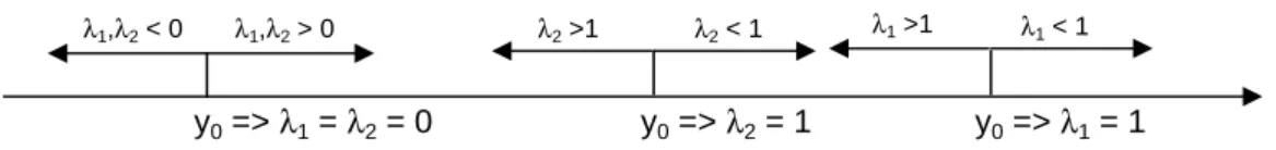
function of y . 0 1 y0 λ1,λ2 A B C λ1 λ2
Figure 4 – The influence of initial output level
In order to have λ1=1 in (23), – point C in figure 4 – the initial level of output must be:
(
)
(
)
(
φ)
µ φ φ γ µ γ φ β α − − + − = 1 1 2 2 0 y , (25)whereas, in order to have λ2 =1 in (24), – point B in figure 4 – the initial level of output must be:
(
)
(
)
(
φ)
φγ φ γ φ ρ β α − − + − = 1 1 2 2 0 y . (26) 22 ( ) (1 ) ( 1) 1 2 0 2 2 2 1 − + − − − = − γ β α φ γ φ φβ α µρµ λ λ y 23As y given by (25) is higher than 0 y given by (26),0 24 this means that for
(
)
(
)
(
φ)
µ φ φ γ µ γ φ β α − − + − > 1 1 2 2 0 y , (27) 1 1<λ and, therefore, also that λ2 <1. Moreover,
φ γ β α − − > 1 1 2 0 y (28)
guarantees that both λ1,λ2 are positive. See point A in figure 4. After noticing that y 0
given by (25) is higher than y given by (28),0
25
it is possible to consider an initial condition
(
)
(
)
(
φ)
µ φ φ γ µ γ φ β α − − + − > 1 1 2 2 0 y , (29)such that it is impossible to associate all the observed behaviours to the correct type of government. In all the other cases, the classification task can be resolved by the perceptron. See figure 5.
y0 => λ1 = λ2 = 0 y0 => λ2 = 1 y0 => λ1 = 1
λ1,λ2 > 0
λ1,λ2 < 0 λ2 >1 λ2 < 1 λ1 >1 λ1 < 1
Figure 5 – The classification regions
Notwithstanding that conditionally, there is a fundamental exception. When output does not show any persistence over time, i.e.
φ
=0, which is, indeed, the most considered case in the literature, it is possible to show that a straight line with intercept between(
2)
2βγ
γρ
−α
and µ µ γ βγ α2 −2and slope equal to α
(
γ +1)
will always divide the space in a correct way, this being eventually the result of the perceptron classification. See the Annex.Plainly, in practical terms, given that a learning process takes place, from the training of
24 ( ) ( ) ( ) ( () )( ) ( ) ( ) 0. 1 1 1 1 1 1 2 2 2 2 2 2 > − − − = −+ − − − − − + − φ φµ µρ γ φ β α φ φγ φ γ φ ρ β α µ φ φ φ γ µ γ φ β α 25 ( ) ( ) ( ) ( ( )) 0. 1 1 1 1 1 2 2 2 2 2 > − − = − − − − − + − φ φµφ γ β α φγ β α µ φ φ φ γ µ γ φ β α
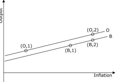
the perceptron does not usually result a straight line with the above mentioned characteristics. Most importantly, given that the two straight lines connecting the two pairs of points in the output-inflation space are parallel, this guarantees that the space is linearly separable. Figure 6 shows this situation.
O u tpu t Inflation (B,1) (B,2) (O,2) (O,1) B O
Figure 6 – A particular(ly interesting) case
As it is well known, if the space can be linearly separable, as it is the case when output does not show any persistence, the perceptron will always determine a vector of values for the weights and a bias value such that the straight line associated with these values divide the space in a correct way. By the use of MATLAB, a simple exercise was performed, whose results are shown in figure 7.
0 0.02 0.04 0.06 0.08 0.1 0.12 0.14 -5 0 5 10x 10 -3 Vectors to be Classified P(1) P (2 )
5. Concluding Remarks
This paper explores a crucial aspect in the issues of political business cycles by considering the effects of bounded rationality, an aspect that has been largely ignored. I hope that this paper has contributed to fill some, even if in a little amount, of the gap.
As a direction for future improvements I would like to explore the possible dynamics of convergence for output in order to check, for the long-run, the real importance of the initial level of output. Furthermore, other types of neural networks may also be considered.
References
BARRELL, Ray, Guglielmo Maria CAPORALE, Stephen HALL, and Anthony GARRATT
(1992), “Learning about Monetary Union: An Analysis of Boundedly Rational Learning in European Labour Markets”, National Institute of Economic and Social Research
Discussion Paper No. 22, August.
BAŞAR, Tamer, and Mark H. SALMON (1990a), “Inflation and the Evolution of the
Credibility with Disparate Beliefs”, in CHRISTODOULAKIS, N.M. (ed.), Dynamic
Modelling and Control of National Economies 1989: Selected papers from the 6th IFAC Symposium, Pergamon Press, Oxford, 75-81.
BAŞAR, Tamer, and Mark SALMON (1990b), “Credibility and the Value of Information
Transmission in a Model of Monetary Policy and Inflation”, Journal of Economic
Dynamics and Control, 14, 97-116.
CHO, In-Koo, and Thomas J. SARGENT (1996), “Neural Networks for Encoding and
Adapting in Dynamic Economies”, in AMMAN, Hans M., David A. KENDRICK, and John
RUST (eds.), Handbook of Computational Economics, Vol. I, Elsevier Science,
Amsterdam, 441-470.
CRIPPS, Martin (1991), “Learning Rational Expectations in a Policy Game”, Journal of
Economic Dynamics and Control, 15, 297-315.
ELLACOTT, Steve, and Deb ROSE (1996), Neural Networks: Deterministic Methods of Analysis, International Thomson Computer Press, London.
EVANS, George W. (1986), “Selection Criteria for Models with Non-uniqueness”,
Journal of Monetary Economics, 18, 147-157.
Rationality and Expectational Stability”, Games and Economic Behavior, Special Issue
on Learning Dynamics, 5, October, 632-646.
EVANS, George W., and Seppo HONKAPOHJA (1994), “Learning, Convergence, and
Stability with Multiple Rational Expectations Equilibria”, European Economic Review,
38, 1071-1098.
EVANS, George W., and Seppo HONKAPOHJA (1995), “Expectational Stability and
Adaptive Learning: An Introduction”, in KIRMAN, Alan, and Mark SALMON (eds.), Learning and Rationality in Economics, Basil Blackwell, Oxford, 102-126.
FUHER, J.C., and M.A. HOOKER (1993), “Learning about Monetary Regime Shifts in an
Overlapping Wage Contract Model”, Journal of Economic Dynamics and Control, 17,
Issue 4, July, 531-553.
GÄRTNER, Manfred, (1996), “Political business cycles when real activity is persistent”,
Journal of Macroeconomics, 18, 679-692.
GÄRTNER, Manfred (1997), “Time-consistent monetary policy under output
persistence”, Public Choice, 92, 429-437.
GÄRTNER, Manfred (1999), “The Election Cycle in the Inflation Bias: Evidence from
the G-7 countries”, European Journal of Political Economy, 15, 705-725.
GÄRTNER, Manfred (2000), “Political Macroeconomics: A Survey of Recent
Developments”, Journal of Economic Surveys, 14, Issue 5, 527-561.
JONSSON, Gunnar (1997), “Monetary Politics and Unemployment Persistence”, Journal
of Monetary Economics, 39, 2, June, 303-325.
MARCET, Albert, and Thomas J. SARGENT (1988), “The Fate of Systems With “Adaptive” Expectations”, The American Economic Review (Papers and Proceedings),
78, No. 2, May, 168-172.
MARCET, Albert, and Thomas J. SARGENT (1989a), “Convergence of Least Squares
Learning Mechanisms in Self-Referential Linear Stochastic Models”, Journal of
Economic Theory, 48, No. 2, August, 337-368.
MARCET, Albert, and Thomas J. SARGENT (1989b), “Convergence of Least-Squares
Learning in Environments with Hidden State Variables and Private Information”,
Journal of Political Economy, 97, No. 6, 1306-1322.
MARIMON, Ramon, and Shyam SUNDER (1993), “Indeterminacy of Equilibria in a
Hyperinflationary World: Experimental Evidence”, Econometrica, 61, No. 5,
1073-1108.
MARIMON, Ramon, and Shyam SUNDER (1994), “Expectations and Learning under
Alternative Monetary Regimes: An Experimental Approach”, Economic Theory, 4,
MINFORD, Patrick (1995), “Time-Inconsistency, Democracy, and Optimal Contingent
Rules”, Oxford Economic Papers, 47, No. 2, April, 195-210.
NORDHAUS, William D. (1975), “The Political Business Cycle”, The Review of
Economic Studies, 42(2), No. 130, April, 169-190.
SALMON, Mark (1995), “Bounded Rationality and Learning: Procedural Learning”, in KIRMAN, Alan, and Mark SALMON (eds.), Learning and Rationality in Economics,
Basil Blackwell, Oxford, 236-275.
SARGENT, Thomas J. (1993), Bounded Rationality in Macroeconomics, Clarendon
Press, Oxford.
SWINGLER, Kevin (1996), Applying Neural Networks: A Practical Guide, Academic
Press Limited, London.
WALL, Kent D. (1993), “A Model of Decision Making Under Bounded Rationality”,
Journal of Economic Behavior and Organization, 20, 331-352.
WESTAWAY, Peter (1992), “A Forward-Looking Approach to Learning in
Macroeconomic Models”, National Institute Economic Review, 2, May, 86-97.
WHITE, Halbert (1989), “Some Asymptotic Results for Learning in Single
Hidden-Layer Feedforward Network Models”, Journal of the American Statistical Association,
Annex – Mathematical details
In the case π0 =αβ , the solutions are:
(
)
(
)
1 1 Bπ
=αβ
−ρ γ φ
− , 1 0 2(
1(
)
)
B y =φy +α β −ρ γ φ γ− − , 2 Bπ
=αβ
, y2B =φ
2y0+α β φ
2(
−2φργ ρφ φγ
+ 2− + − +1γ γ ρ
2)
, 1 1 O γ φ π αβ µ − = − , 2 1 0 O y φy α β µ γ φ γµ µ − + − = + , 2 Oπ
=αβ
, 2 2 0 1 O y φ φy α β µ γ φ γµ α αβ γαβ γ φ µ µ − + − − = + + − − .This means that:
(
)
1 1 1 B O µρ π π αβ γ φ µ − − = − ,π
2B−π
2O=0,(
)
2 1 1 1 B O y y α β γ φ µρ µ − − = − , y2B y2O α β γ φ2(
)
21 µρ µ − − = − − .Given the previous expressions, the slopes and intercepts of the straight lines, yti = +ai bi
π
ti, for i = B,O and t = 1,2 are:( )
(
)
( ) 2 2 2 0 1 y 2 Bb
=
φ φ− +α β γφ γ ρ φργ ργ ρφ φ ρφ− +βαρ γ φ−− + + + − ,(
)
(
)
( ) 2 2 2 2 2 2 2 2 2 2 2 3 3 2 0 1 y 4 2 2 3 3 Ba
=
φ − + +φ ρφ φργ− +α β φργ γρφ φ φργ− + − φ γ ρ− + ρφ γφ γ ρ φρ γ− + + − φ ρ γ ρ φ γ ρ+ − , ( )(
)
( ) 2 2 2 0 1 y 2 Ob
=
φµ φ− −α β φγµ γβα γ φ− +− γφ γ φ φµ φ− − − + ,(
)
(
)
( ) 2 2 2 2 3 3 2 2 2 2 2 2 0 4 3 3 2 2 y Oa
=
µφ φ φµ γφ µ+ − − −α β φγµ φγ− + φ γ γ φφ γ µ−+ − − µγ µ φγ µφ γ µφγ µ φ φ µ+ + − − − .Those two lines will cross at
(
)
(
)
(
)
(
)
3 2 2 0 1 1 y 1α βρ φ γ
π αβ
φ
α β
γ µφ
− = − − + − .Moreover,
(
) (
1)
0(
2)
(
1)
1 B O y b bφ
ρµ
φ
α β γ
αβρ γ φ
− − − − = − − ,(
)
(
1)
0 2(
(
)
3 3 2 3 2 3)
1 B O y a aρµ
φµ
φ
α β φµ φγµ ργ
φργ
γρφ φ ρ
γ φ µρ
− + − + − + − + − = − − .In the particular case of an initial output level 0 2 1
1 y
α β
γ
φ
− = − we have(
1)
0 B O b =b =α
− +φ γ
> ,(
)
( )2 2 1 0 B O a −a = − −ρµ α β
γ φ−µ < .In case of no persistence at the output level, that is when
φ
=0, the solutions are:(
)
1 1 Bπ
=αβ
−ργ
,π
2B =αβ
,(
)
2 1 1 B y =α β
− −γ γρ
, y2B =α β
2(
1− +γ γ ρ
2)
, 1 1 Oγ
π
αβ
µ
= − , 2 Oπ
=αβ
, 2 1 O yα β
µ γ γµ
µ
− − = , 2 2 2 O yα β
µ γ
γµ
µ
+ − = .It is then straightforward to verify that:
1 1 1 0 B O
µρ
π
π
αβγ
µ
− − = > , 2 2 0 B Oπ
−π
= ,(
)
2 2 1 1 0 B B y −y =α βγ
+γ ρ
> , 2 1 2(
)
1 1 0 O O y yα βγ
γ
µ
− = + > , 2 1 1 1 0 B O y yα βγ
µρ
µ
− − = > , 2 2 2 21 <0 − − = −µ
µρ
βγ
α
O B y y , 2 2 1 0 O B y yα βγ
γ µρ
µ
+ − = > .for i = B,O and t = 1,2 are: