UNCORRECTED
PROOF
12
3 ORIGINAL PAPER
4
A case study of Eucalyptus globulus fingerprinting
5
for breeding
6 Maria Margarida Ribeiro&Leopoldo Sanchez& 7 Carla Ribeiro&Fátima Cunha&José Araújo&
8 Nuno M. G. Borralho&Cristina Marques
9 Received: 17 August 2010 / Accepted: 21 December 2010 10 # INRA and Springer Science+Business Media B.V. 2011 11
12 Ab
Q2 stract
13 & Introduction Tree genetic improvement programs usually 14 lack, in general, pedigree information. Since molecular 15 markers can be used to estimate the level of genetic 16 similarity between individuals, we genotyped a sample of a 17 Portuguese Eucalyptus globulus breeding population—a 18 reference population of 125 individuals—with 16 micro-19 satellites (SSR).
20 & Materials and methods Using genotypes from the
21 reference population, we developed a simulation approach 22 to recurrently generate (105 replicates) virtual offspring 23 with different relatedness: selfed, half-sib, full-sib and
24
unrelated individuals. Four commonly used pairwise
sim-25
ilarity coefficients were tested on these groups of simulated
26
offspring. Significant deficits in heterozygosity were
27
found for some markers in the reference population,
28
likely due to the presence of null alleles. Therefore, the
29
impact of null alleles in the relatedness estimates was
30
also studied. We conservatively assumed that all
31
homozygotes in the reference population were carriers
32
of null alleles.
33
& Results All estimators were unbiased, but one of them
34
was better adjusted to our data set, even when null alleles
35
were considered. The estimator’s accuracy and precision
36
were validated with individuals of known pedigree obtained
37
from controlled crosses made with the same reference
38
population’s parents. Additionally, a clustering algorithm
39
based on the estimator of choice was constructed, in order to
40
infer the relatedness among 24 E. globulus elite individuals.
41
We detected four putatively related elite individuals’ pairs
42
(six pairs considering the presence of null alleles).
43
&Conclusions This work demonstrates that in the absence
44
of pedigree information, our approach could be useful to
45
identify relatives and minimize consanguinity in breeding
46
populations.
47
Keywords Microsatellites . Eucalyptus globulus . Null
48
alleles . Relatedness
49
1 Introduction
50
Eucalyptus globulus ssp. globulus (hereafter E. globulus) is
51
an economically important species for pulpwood
produc-52
tion, actively bred in many countries (Eldridge et al.1994),
53
including Portugal, where the first formal breeding program
54
for the species began in 1966 (Borralho et al.2007). In general,
Handling Editor: Christophe Plomion
Electronic supplementary material The online version of this article (doi:10.1007/s13595-011-0087-x) contains supplementary material, which is available to authorized users.
M. M. Ribeiro (*)
Departamento de Recursos Naturais e Desenvolvimento Sustentável, Escola Superior
Q1 Agrária,
6001-909 Castelo Branco, Portugal e-mail: [email protected]
L. Sanchez
INRA Centre d’Orléans, Unité Amélioration, Génétique et Physiologie Forestière, 45166 Olivet, France
e-mail: [email protected] C. Ribeiro
:
F. Cunha:
J. Araújo:
C. Marques RAIZ-Direcção de Investigação Florestal, Herdade de Espirra, 2985-270 Pegões, Portugal N. M. G. Borralho BorralhoIDea, Urbanização S. Francisco, 18, 2070-220 Cartaxo, Portugal Annals of Forest Science DOI 10.1007/s13595-011-0087-xUNCORRECTED
PROOF
55 the foundation of breeding populations aims to capture, as56 close as possible, the genetic diversity of the original 57 population. However, breeding activities will rapidly reduce 58 genetic diversity due to selection intensity, linkage and 59 random drift in finite populations (Lefèvre2004). Moreover, 60 inbreeding depression is known to be severe in this species 61 (Hardner and Potts 1995; Costa e Silva et al. 2010). To 62 ensure that levels of coancestry and inbreeding among 63 selected trees are kept to a minimum, it would be 64 advantageous to know the relatedness among parents of 65 unknown pedigree
Q3 , particularly in early stages of breeding
66 programs (Ballou and Lacy 1995). In the absence of 67 known pedigree information, estimates of relatedness 68 between individuals can be obtained through the use of 69 molecular markers. Codominant microsatellite markers 70 (SSR) are particularly suitable for this purpose, as they 71 can be used to estimate individuals’ pairwise relatedness, 72 based on probability ratios of identity in state between 73 individuals and an unrelated reference population. These 74 estimates are very useful to infer the level of relatedness 75 among sub-populations of elite material, to assure the 76 deployment of unrelated elite clones and/or for the 77 design of controlled crosses between putatively unrelated 78 parents.
79 Estimators of pairwise relatedness were first consid-80 ered for DNA data by Lynch (1988). This first estimator 81 was modified by Li et al. in order to accommodate 82 codominant markers (1993). Band sharing by chance is 83 difficult to separate from band sharing by descent, and a 84 method-of-moments (MM) estimator for pairwise related-85 ness was developed by Queller and Goodnight (1989). 86 Afterwards, more accurate and precise MM estimators 87 were developed by Ritland (1996) and Lynch and Ritland 88 (1999). Recently, Wang (2002) introduced a new estima-89 tor, an improved version of the one proposed by Li et al. 90 (1993), but Csillery et al. (2006) demonstrated that its 91 performance was poor. Other estimators, including max-92 imum likelihood methods (ML), were proposed to esti-93 mate relatedness in the absence of known pedigree 94 structure (Queller and Goodnight 1989; Li et al. 1993; 95 Lynch and Ritland 1999; Wang 2002; Milligan 2003; 96 Thomas 2005; Oliehoek et al. 2006) and were used in 97 different areas of research (reviewed by Blouin 2003 and 98 Thomas 2005). Their performance was compared in 99 several studies using simulated and empirical datasets 100 (Lynch and Ritland 1999; Van de Casteele et al. 2001; 101 Wang 2002; Milligan 2003; Csillery et al. 2006). These 102 studies agree in that no single estimator is universally 103 superior to the others in terms of bias and variance and 104 that the performance rank order of the estimators depends 105 on the estimation of the true relatedness value, the 106 informativeness of the markers (number of loci and number 107 and frequencies of alleles per locus) and the sample size used
108
to estimate allele frequencies. For the commonly available
109
markers in most studies (∼ 5 to 20 microsatellites), the
110
MM estimators are preferred because the ideal
proper-111
ties of ML methods are only achieved asymptotically
112
(Lynch and Ritland 1999; Wang 2002; Milligan 2003).
113
Additionally, the presence of null alleles in SSR markers
114
can introduce a bias in the estimation of relatedness
115
(Wagner et al. 2006). However, little is known on the
116
actual impact of null alleles on the behaviour of relatedness
117
estimators.
118
In this study, we compared three commonly used MM
119
coefficients to estimate pairwise similarity: Ritland
120
(1996) (R), Queller and Goodnight (1989) (Q) and Lynch Q4
121
and Ritland (1999) (LR), and a band sharing method: Li et
122
al. (1993) (L), in the context of a Portuguese E. globulus
123
breeding population. We followed a Monte Carlo
simula-124
tion strategy and, unlike previous studies in the literature,
125
considered two different criteria to identify the best
126
performing estimator: (1) smaller average overlapping
127
areas between every two density distribution relatedness
128
categories and (2) smaller impact from the presence of
129
null alleles.
130
We have used 16 publicly available SSR markers to
131
screen 125 putatively unrelated individuals from an elite
132
breeding population of E. globulus. The assumption of
133
Hardy–Weinberg equilibrium in breeding populations of
134
artificial origin might not hold true. However, this issue
135
was overcome by measuring relatedness on the randomly
136
generated in silico individuals from the existing parents in
137
the reference breeding population.
138
In order to define a threshold to transform the continuous
139
range given by the pairwise methods into genealogical
140
relatedness (e.g. Blouin et al. 1996; Kozfkay et al.2008),
141
the density distributions of the simulated selfed, half-sib,
142
full-sib and unrelated offspring were obtained. The selected
143
threshold corresponds to the interception of the probability
144
distribution curves of the unrelated and the half-sib
145
individuals. This critical value is only coincident with the
146
cut-off defined by Blouin et al. (1996) when the density Q5
147
distributions are absolutely symmetric, which is not always
148
the case (e.g. Kozfkay et al. 2008). An additional
149
population of 24 elite trees from the genetic improvement
150
program was genotyped, as a practical application of the
151
methodology developed here.
152
The objectives of this study are to provide estimates
153
of the genetic parameters of the SSR used, including its
154
discriminant power (D), to select the better suited
155
relatedness estimator across unrelated (UR), half-sib
156
(HS), full-sib (FS) and individuals generated by selfing a
157
single parent (SF), to validate the estimator’s precision and
158
accuracy with individuals of known pedigree (HS, FS and SF),
159
and to study the impact of null alleles in the relatedness
160
estimates.
M.M. Ribeiro et al.
JrnlID 13595_ArtID 87_Proof# 1 - 15/05/2011
was modified by Li et al. in order to accommodate was modified by Li et al. in order to accommodate
UNCORRECTED
PROOF
161 2 Material and methods162 2.1 Plant material and DNA extraction
163 The E. globulus population of 125 putatively unrelated 164 individuals (hereafter reference population, RP), includes 165 12 individuals used in controlled crosses to produce the 166 validation population. The remaining 113 were putatively 167 unrelated E. globulus individuals representative of the 168 genetic improvement population of RAIZ (Forestry and 169 Paper Research Institute, Portugal) (Borralho et al. 2007). 170 This group includes 47 trees originally selected in planta-171 tions in Portugal (referred herein as “Portuguese land race”) 172 and 66 trees from 13 Australian native races (classification 173 follows Dutkowski and Potts (1999). The validation 174 population comprised three half-sib families, three full-sib 175 families and four selfed families (each family with 176 individuals generated by selfing a single parent), from 177 controlled crosses made between 12 putatively unrelated 178 individuals of the Portuguese land race. Each family had six 179 offspring. An extra set of 24 elite clones was also 180 genotyped. These 24 elite trees were used as a practical 181 application of the proposed methodology. They were 182 selected from RAIZ E. globulus breeding population and 183 are to be used for deployment. Total genomic DNA was 184 extracted as in Marques et al. (1998). DNA concentration 185 was estimated by comparison of the fluorescence intensities 186 of ethidium bromide-stained samples to those of λDNA 187 standards, on 1% agarose gels.
188 2.2 SSR, PCR conditions and sizing of PCR products 189 Sixteen publicly available eucalypt SSR (Appendix 11) 190 were selected for its allele number and effective number of 191 alleles (Table 1). SSR primer design was described 192 elsewhere (EMBRA 1–20 in Brondani et al (1998), 193 EMCRC1-12 in Steane et al. (2001) and EMBRA 21–70 194 in Brondani et al. (2002)). Each SSR marker was 195 assigned to a consensus linkage group based on E. 196 globulus genetic linkage maps (unpublished results) and 197 a consensus map of a Eucalyptus grandis × Eucalyptus 198 urophylla pedigree (Brondani et al. 2006). EMCRC5 was 199 the only unmapped marker in this study. Three SSR 200 (EMBRA 6, EMBRA 11 and EMBRA 12) mapped to the 201 same linkage group (no. 1, see Appendix 1), but in 202 different locations (unpublished results). The remaining 203 seven SSR mapped to different linkage groups. Despite 204 the fact that we expect high SSR synteny in the eucalypt 205 Symphyomyrtus subgenus (Marques et al. 2002), we 206 performed linkage disequilibria tests for all loci
combina-207
tions with the Genepop version 4.0.7 (Rousset2008). The
208
p values were obtained by the contingency table approach
209
(Fisher’s exact test), and the number of dememorization
210
steps was 10,000, with 1,000 batches and 100,000 iterations
211
per batch. The significance level, with a probability of type I
212
error of 1%, took into account the number of tests performed
213
by using the Bonferroni correction (Sokal and Rohlf1997).
214
The Hardy–Weinberg test was made by estimating the exact
215
p values by the Markov chain method, with the same
216
dememorization steps, batches and iterations per batch
217
referred in the foregoing. The null allele frequencies per
218
loci were estimated by using a maximum likelihood EM
219
algorithm. Both were computed with the Genepop software.
220
Polymerase chain reaction amplification of SSR loci
221
was carried out in 96-well V-bottom plates. Each reaction
222
contained 0.2, 0.15 and 0.1 μM of primer (for SSR in
223
groups 1, 2 and 3, respectively—Appendix 1), 0.5 U of
224
Taq DNA polymerase (Promega, Madison, WI, USA),
225
0.2 mM of each dNTP (otherwise as specified in
226
Appendix 1, Promega, Madison, WI, USA), 1× reaction
227
buffer (Promega, Madison, WI, USA), 2 mM of MgCl2 228
(Promega, Madison, WI, USA), DMSO 5.0% (Sigma)
229
and 20 ng of template DNA in a final 10-μl volume.
230
Forward primers were IRD800 (5′-fluoresceine) labelled.
231
Reactions were cycled in an MJ Research PT-100
232
Thermal Controller with a heated lid, 94°C for 30 s,
233
followed by 15 cycles of variable annealing temperature
234
(“touch down”): 94°C for 30 s, 30 s of annealing
235
(from 56°C, with a decrease of 0.2°C every cycle), and
236
72°C for 45 s; then 20 cycles of 94°C for 30 s, 53°C
237
for 30 s and 72°C for 45 s; and finally 72°C for 7 min.
238
Amplification products were denatured by adding 10 μL of
239
formamide buffer (98% formamide deionized, 10 mM EDTA
240
pH 8.0, 60 mg bromophenol blue), heated 5 min at 70 C
241
(Termomixer Confort, Eppendorf), and 0.8 μL of the
242
samples was loaded in 6% acrylamide denaturating gel
243
(50% Long-Ranger , with 10.5 g Urea and 2.5 ml TBE
244
(10×)). Fragments were separated using a LI-COR automatic
245
DNA sequencer (model 4200 Gene Readir) at 1,500 V, 25 W
246
constant power, 45°C of plate temperature and a 1× TBE
247
running buffer, for approximately 2 h. RFLPscan was used to
248
retrieve the gel image, and the presence of the bands was
249
visually scored with the help of a LA4000-44B LI-COR
250
ladder.
251
2.3 Relatedness estimators
252
The coancestry coefficient (θ) between individuals x and y
253
is the probability that two randomly chosen homologous
254
alleles are identical ‘by descent’ (Lynch and Walsh1998).
255
In a diploid mating system, the coefficient of coancestry
256
multiplied by 2 equals the coefficient of relatedness, rxy, 257
which is the expected fraction of alleles identical by
1
Appendix is available online only atwww.asf-journal.org. Eucalypt’s fingerprinting for breeding
JrnlID 13595_ArtID 87_Proof# 1 - 15/05/2011
). The validation ). The validation
UNCORRECTED
PROOF
258 descent between two (related) individuals. Alleles are259 identical by descent if they recently descend from a 260 single ancestral allele. Alleles that are identical by state 261 (IBS) might not be identical by descent if they coalesce 262 further back than the reference pedigree or arose 263 independently via mutation (see Blouin 2003for details). 264 In fact, the estimated relatedness measures how much 265 higher (or lower) the probability of recent coalescence is 266 for any given pair (x, y), relative to the average probability 267 for all pairs. The expected relatedness is 0.67 for selfed, 268 0.5 for full-sibs, 0.25 for half-sibs and 0 for unrelated 269 individuals. For example, on average, a pair of siblings 270 (FS) shares one out of two alleles identical by descent 271 (Squillace1974; Falconer and Mackay1996; Blouin2003). 272 Lynch (1988) relatedness estimator based on band 273 sharing and modified by Li et al. (1993) (L) is:
rxy¼ sxy s0 1 s0 and s0¼ Xn i¼1 p2ið2 piÞ; ð1Þ 274
275 where Sxyis the similarity index Sxy=nxy/2(1/nx+1/ny), nxy 276 is the number of shared alleles between individuals x and y,
277 nxis the number of alleles of x, nyis the number of alleles 278 of y and S0is the number of shared alleles in the reference 279 population, based on the allele frequencies (pi is the 280 frequency of the ith allele).
281
Ritland (1996) (R) coancestry estimator of individuals X=
282
(A1,A2) and Y=(A3,A4) can be written as: qxy¼ 1 4 nð i 1Þ # dðA1;A3Þ þ d Að 1;A4Þ p Að 1Þ ! " þ dðA2;A3Þ þ d Að 2;A4Þ p Að 2Þ ! " 1 # $ ð2Þ 283 284
where δ, the Kronecker operator, is defined for alleles Aiand 285
Aj: δ(Ai,Aj)=1 if Ai=Aj, and δ(Ai,Aj)=0 if Ai≠Aj. We have six 286
operators to compare two individuals (two within and four
287
between individuals) in the same locus, p(Ai) being the 288
frequency of the Ai allele in the considered locus and
289
reference population and nithe total number of alleles in the 290
considered locus and reference population (Ritland2000).
291
The Queller and Goodnight (1989) (Q) relatedness
292
estimator is based on the same Kronecker operator and is
293 described as: rxy¼ dðA1;A3Þ þ d Að 1;A4Þ þ d Að 2;A3Þ þ d Að 2;A4Þ p Að 1Þ p Að 2Þ ð Þ 2 1ð þ d Að 1;A2Þ p Að 1Þ p Að 2ÞÞ ð3Þ 294 295 296
Still based on Kronecker operators, Lynch and Ritland
297
(1999) developed another relatedness estimator (LR) which
298 is defined as follows: 299 300 301 rxy¼ p Að 1Þd Að 2;A3Þ þ d Að 2;A4Þ ð Þ þ p Að ð 2Þd Að 1;A3Þ þ d Að 1;A4ÞÞ 4 pAð 1Þp Að 2Þ 1þ d Að 1;A2Þ ð Þ p Að ð 1Þ þ p Að 2ÞÞ 4p Að 1Þp Að 2Þ ð4Þ 302 303 304 t1.2 Na Ne He Ho Fis Sig. Null D t1.3 EMBRA23 21 12.8 0.93 0.89 0.04 NS 0.031 0.991 t1.4 EMBRA12 19 13 0.93 0.89 0.04 NS 0.025 0.991 t1.5 EMCRC8 18 12.8 0.93 0.84 0.09 S 0.049 0.987 t1.6 EMBRA18 21 11.5 0.92 0.90 0.01 NS 0.011 0.987 t1.7 EMCRC11 16 8.9 0.89 0.83 0.07 NS 0.032 0.981 t1.8 EMBRA6 15 8.8 0.89 0.78 0.12 S 0.055 0.976 t1.9 EMCRC10 18 8.6 0.89 0.65 0.26 S 0.130 0.960 t1.10 EMBRA11 21 9.4 0.90 0.87 0.02 NS 0.029 0.960 t1.11 EMBRA2 15 6.2 0.84 0.76 0.1 NS 0.044 0.959 t1.12 EMBRA8 14 6.2 0.84 0.76 0.1 NS 0.046 0.956 t1.13 EMCRC7 14 4.8 0.79 0.70 0.11 NS 0.048 0.932 t1.14 EMBRA20 13 4.7 0.79 0.62 0.21 S 0.091 0.929 t1.15 EMCRC2 15 4.5 0.78 0.62 0.2 S 0.107 0.915 t1.16 EMBRA5 21 5.2 0.82 0.50 0.34 S 0.158 0.898 t1.17 EMCRC5 21 5.5 0.81 0.53 0.37 S 0.165 0.898 t1.18 EMBRA19 6 3.4 0.71 0.54 0.24 S 0.155 0.855 t1.19 Mean 16.8 7.9 0.85 0.73 0.15 0.074 0.948
t1.1 Table 1 Diversity parameters
Q6
for the 16 SSR loci in the reference population, ordered according to its discriminant power (D)
Sig. refers to the significance resulting from the HWE test (after Bonferroni correction, where NS means not significant and S significant), and null refers to null allele frequency estimates
Nanumber of alleles per locus,
Ne effective number of alleles,
He expected heterozygosity, Ho
observed heterozygosity, Fis
fixation index
M.M. Ribeiro et al.
UNCORRECTED
PROOF
305306 2.4 Estimation of genetic parameters and simulation 307 methods
308 For each SSR locus in the RP, the number of alleles (Na), 309 the effective number of alleles (Ne=1/(1 −He)), the observed 310 heterozygosity (Ho) and the expected heterozygocity 311 (He) (Nei 1987) were computed with a FORTRAN 312 program developed in this study, hereafter called Zeta 313 (available upon request from LS). The fixation index 314 (Fis) (Weir and Cockerham1984) was estimated with the 315 Genepop software version 4.0.7.
316 The distribution of relatedness r-values estimated with 317 the L, R, Q and LR coefficients was obtained by generating 318 105 replicates of UR, HS, FS and SF individuals, from 319 where mean and sampling variance values were calculated. 320 Each replicate consisted of two in silico individuals. These 321 individuals were obtained assuming free recombination and 322 segregation out of parental SSR genotypes. Parents were 323 sampled at random. In the UR group, four distinct parents 324 were sampled and single-pair mated in order to obtain two 325 unrelated offspring. For the HS group, three distinct parents 326 were sampled, and one of them mated to the other two, in 327 order to obtain one offspring from each mating. With the 328 FS group, only two parents were sampled and mated, in 329 order to obtain two full-sib individuals. Finally, in the SF’s 330 group, one parent was sampled and selfed twice, in order to 331 get two offspring.
332 The relatedness between any two in silico individuals, 333 measured in each replicate, the r-value (rxy), was computed 334 using a weighted multilocus average:
rxy¼
P
i
rxyðiÞ Var rxyðiÞ
& ' (
P
i
1 Var r( & xyðiÞ'
;
335
336 where rxy(i) is the estimator’s value for the ith locus, 337 according to one of the four estimators (L, R, Q or LR, in
338 Eqs.1,2,3 or4, respectively), and Var
Q7 (rxy(i)) is the Monte
339 Carlo sampling variance for the same locus over
340 replicates, which was used as a weighting factor for
341 the multilocus average. Therefore, variable loci will
342 account for less in the average, compared to less
343 variable loci. A sampling variance was also calculated
344 for the multilocus average (Var rxy), as the Monte Carlo
345 variance over replicates.
346 In order to evaluate the informativeness of each SSR 347 marker for fingerprinting, we estimated its discriminant 348 power (D) by using Zeta. D was the number of replicates in 349 which a given marker was able to discriminate between two 350 simulated individuals with a given level of relatedness, over 351 the total number of 105replicated pairs. The discriminant 352 power was obtained for each marker and for each
353
relatedness group. This indicates the likelihood of
discrim-354
ination of any two individuals derived from the reference
355
population, over relatedness classes.
356
To study the impact of null alleles, we assumed an
357
extreme simulation scenario where each putative
homozy-358
gote in the RP was a carrier of one null allele. Pairwise
359
relatedness estimators (rxyn) were obtained with the
proce-360
dure explained before and were compared to the
361
corresponding cases without null alleles.
362
From each r-value distribution obtained from Zeta, based
363
on 105replicates, we randomly sampled 10,000 replicates
364
(one tenth) and used them to draw density distributions. For
365
each L, R, Q or LR estimator, we placed the four resulting
366
density distributions from each relatedness group along the
367
same axis and calculated the overlapping areas, i.e. UR–
368
HS, UR–FS, UR–SF, HS–FS, HS–SF and FS–SF. The total
369
overlapped area obtained per relatedness estimator was an
370
indicator of its resolving power in distinguishing among
371
relatedness classes. A similar procedure was carried out
372
assuming null alleles. Based on the density distribution
373
curves, we have also computed the exact percentiles at
374
2.5% and 97.5% to frame the simulated multilocus r-values
375
for each relatedness group and coefficient. Density
distri-376
butions and corresponding overlapping areas were
comput-377
ed with density functions written in the R statistical
378
package (R Development Core Team 2008).
379
Most pairwise methods provide estimates within a
380
continuous range that need to be converted into
genealog-381
ical relatedness (UR, HS, FS and SF). This can be done
382
through the use of arbitrary thresholds between relatedness
383
classes, usually the midpoint between means of two
384
consecutive relatedness classes (e.g. 0.125: UR–HS)
385
(Blouin et al.1996). We established the relatedness groups
386
by looking at the overlapping area between density
387
distributions and defining the relatedness value according
388
to the interception point between any two overlapping
389
distributions. This interception point was taken as the
390
threshold between the two given relatedness classes
391
(subsequently called the ‘critical value’). This critical value
392
minimizes both β and α errors (β is the overlapping area to
393
the left of the critical value and α is the one to the right)
394
(Kozfkay et al.2008). Given that our interest was to know
395
whether a given pair of individuals was unrelated or
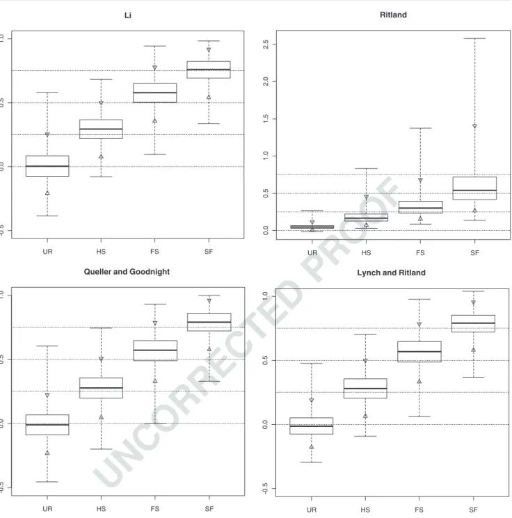
396
related to some extent, only one threshold between UR
397
and the rest of the relatedness classes was obtained per
398
estimator (L, R, Q or LR). The decision of accepting or
399
rejecting the null (H0: ‘the pair are unrelated individuals’) 400
or the alternative hypotheses (H1: ‘the pair are half-sib 401
individuals’) was made comparing the observed r-value to
402
the threshold. The threshold value was used to decide
403
which pairs of the 24 trees from the elite population
404
were related to some extent, at least at the half-sib level
Eucalypt’s fingerprinting for breeding
UNCORRECTED
PROOF
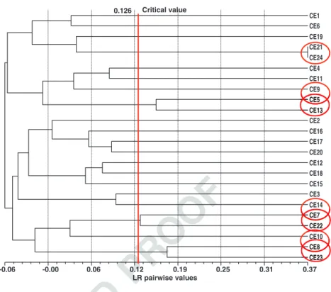
405 (indicated by the comparison of the estimated pairwise406 r-value with the threshold value), using the pairwise LR 407 values (Fig. 5).
408 The relatedness estimator with the smallest percent-409 age of overlapping density probabilities and lower 410 impact from the presence of null alleles was selected 411 for further analysis with the 24 individuals of the elite 412 population.
413 The validation population (three HS, three FS and four SF 414 families) relatedness estimators were calculated using the 415 SPAGeDi version 1.2 software (Hardy and Vekemans2002). 416 The pairwise relatedness matrix of the LR coefficient 417 estimates for the 24 elite clones was used to perform an 418 unweighted pair group method with arithmetic mean 419 (UPGMA) dendogram. The UPGMA tree topology was 420 tested by comparing the elite clones LR pairwise matrix 421 and the correspondent cophenetic matrix through a 422 Mantel test (Sokal 1979). A normalized Z test was 423 performed. The observed value after 1,000 permutations 424 should be significantly larger than that expected by 425 chance, in order for an association to be accepted. 426 NTSYSpc version 2.1 (Rohlf2000) was used to compute 427 the UPGMA and the Mantel test.
428 3 Results 429 3.1 SSR loci
430 The effective number of alleles per loci (Ne) in the reference 431 population ranged from 6 to 21, with an average of 16.8 432 (Table 1). The observed heterozygosity (Ho) values 433 ranged from 0.5 to 0.9. Loci with the same number of 434 alleles (Na) exhibited different effective number of alleles 435 (Ne) and also different discriminant power (D) (loci with 436 21 alleles show Neranging from 5.2 to 12.8, Table 1). As 437 an example, the allele frequency distributions of loci 438 EMBRA5 and EMBRA23 (same Na different Ne) are 439 displayed in Appendix2. Locus EMBRA23 has a more even 440 allele frequency distribution compared to locus EMBRA5, 441 which results in differences in Ne, though they have the same 442 Na. EMBRA5 has few high frequent alleles and many alleles 443 with very low frequencies. Loci that displayed higher 444 values of Na/Nealso showed higher values in He/Horatio 445 (i.e. EMBRA5, EMCRC5, EMBRA20 and EMCRC2) and 446 are among the loci with lowest D.
447 High Fis values—the loss of heterozygosity due to non-448 random mating of parents —reflected differences between 449 observed and expected heterozygosity. We need to note 450 here that the reference population included individuals 451 selected in stands after phenotypic evaluation and without 452 pedigree information. Loci displayed different deviations 453 from Hardy–Weinberg expectations (HWE), and half of
454
them were not under HWE. The presence of null alleles is
455
one complementary hypothesis for departures from HWE.
456
Table 1 shows null allele frequencies above 5% and
457
significant HWE deviations for EMBRA6, EMCRC10,
458
EMBRA20, EMCRC2 EMBRA5, EMCRC5 and
459
EMBRA19. All loci combinations gave non-significant
460
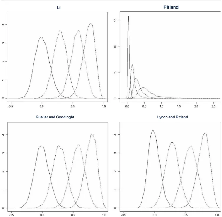
linkage disequilibrium values after the Bonferroni
correc-461
tion. The only locus without mapping information
462
(EMCRC5) appeared not linked to any other marker.
463
Therefore, we assumed that all the markers used in this
464
study have independent segregation.
465
3.2 Relatedness estimators
466
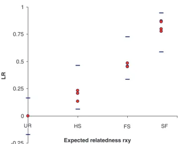
All estimators revealed similar levels of upward bias
467
(the distance between the expected relatedness value and
468
the observed mean) (Fig. 1), more evident in the higher
469
relatedness class (FS and SF). Despite these biases,
470
expected values fell well within exact percentiles at
471
2.5% and 97.5% for all four estimators and relatedness
472
classes. R showed a different behaviour, with overlapping
473
exact percentiles at 2.5% and 97.5% for all the relatedness
474
classes. According to this information, unrelated
individ-475
uals could be distinguished from FS and SF individuals,
476
and HS could be distinguished from SF individuals, for
477
all estimators except R. The LR estimator produced
478
slightly smaller exact percentiles at 2.5% and 97.5%
479
(confidence percentiles = CP) than the Q estimator, in
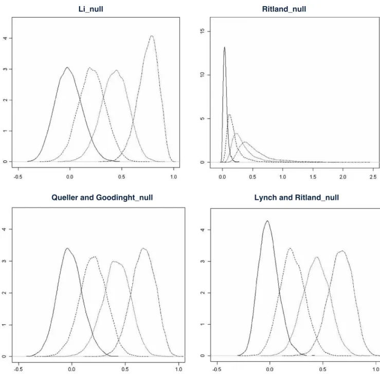
480
particular the UR class. The L estimator had slightly
481
smaller confidence percentiles than LR, but not in the case of
482
the unrelated individuals. Considering the percentage of
483
overlapping areas of the density distributions of r-values
484
(without taking into account the presence of null alleles),
485
on average, the R coefficient had the highest mean
486
overlapping distributions’ area (OD) across relatedness
487
groups (20.8%) and the LR estimator the lowest (11.6%),
488
as shown in Table 2. The percentage of overlapping area
489
was higher, for the comparison between FS–SF (36.5%),
490
followed by the HS–FS and the UR–HS. The lowest
491
OD was found in the UR–SF, with no overlapping
492
areas for LR and Q estimators. Therefore, the
over-493
lapping area for LR was generally the lowest, with the
494
exceptions in the comparison UR–HS where it equalled
495
R and in HS–FS where the L coefficient had a slightly
496
better performance.
497
Considering nonparametric tests the overlapping areas,
498
the worst behaving coefficient is R. LR proved to be the
499
best overall performing relatedness estimator displaying
500
the smallest average percentage of overlapping areas
501
(11.6%), when compared with the other estimators’ ODs
502
(Table 2).
503
In Fig. 2, the density distributions for all relatedness
504
estimators, without null alleles, are represented. L, Q and
M.M. Ribeiro et al.
UNCORRECTED
PROOF
505 LR show approximately similar densities, with LR having a 506 slightly narrower curve for UR. In general, these three 507 estimators show symmetrical curves for UR, with asym-508 metry increasing progressively towards classes with higher 509 relatedness. In SF class of r-values, the right tail is slightly 510 shorter than the left tail, i.e. exhibiting negative skewness. 511 Considering the R estimator, the density curve was 512 extremely leptokurtic for UR r-values, and with increasing
513
platykurtic properties and positive skewness towards
514
classes with higher relatedness.
515
The LR pairwise relatedness values computed for the
516
groups of individuals with known pedigree (SF, full-sibs,
517
half-sibs and unrelated) are shown in Fig.3, together with
518
the corresponding exact percentiles at 2.5% and 97.5%.
519
Observed LR relatedness appears slightly downward biased
520
for half-sib and full-sib groups, while SF shows upward
-0 .5 0 .0 0 .5 1 .0 UR HS FS SF Li 0. 0 0 .5 1. 0 1 .5 2. 0 2 .5 UR HS FS SF Ritland -0 .5 0 .0 0 .5 1 .0 UR HS FS SF
Queller and Goodnight
-0 .5 0 .0 0 .5 1 .0 UR HS FS SF
Lynch and Ritland
Fig. 1 Distribution of simulated multilocus r-values (whiskers for maxima and minima, triangles for exact percentiles at 2.5% and 97.5%, bottom and top of the box for the lower and upper quartiles, respectively, and band near the middle of the box for the median) in the different relatedness groups (unrelated, half-sibs (HS), full-sibs
(FS) and individuals generated by selfing a single parent (SF) for different relatedness/coancestry estimators: Li et al. (1993) (L), Ritland (1996) (R), Queller and Goodnight (1989) (Q) and Lynch and Ritland (1999) (LR)
Eucalypt’s fingerprinting for breeding
JrnlID 13595_ArtID 87_Proof# 1 - 15/05/2011
(unrelated, (unrelated,
by selfing a single parent (SF) for by selfing a single parent (SF) for
UNCORRECTED
PROOF
521 estimates, when compared to theoretical expectations. All522 observed estimates fell within the exact percentiles at 2.5% 523 and 97.5%. Additionally, LR was also calculated for the 524 reference population of 125 putatively unrelated trees. 525 Results not shown graphically here indicate that 4.4% of 526 relatedness fell beyond what would be expected to be the 527 upper bound for unrelated pairs, based on the 97.5% exact 528 percentile for UR, with a β error of 8%.
529 3.3 Impact of null alleles on relatedness estimators 530 ODs per relatedness coefficient and across relatedness 531 classes when null alleles were assumed are shown in 532 Table 2. In general, the inclusion of null alleles led to 533 increases in OD, making it more difficult to differentiate the 534 four relatedness classes through the use of the estimators. 535 Only a few cases involving SF with L exhibited lower OD 536 with null alleles than without them. Considering the 537 resulting ODs per estimator, R remained the one with the 538 highest overlapping areas amongst density distributions of 539 r-values. The other three estimators had similar ODs, with 540 L showing the smallest, closely followed by LR, and Q 541 being the second largest.
542 Density distributions are represented for all relatedness 543 estimators with null alleles in Fig. 4. In general, the 544 inclusion of null alleles led to distributions of larger 545 variances and correspondingly broader bell shapes. As a 546 consequence of that, the overlapping areas were larger 547 under the hypothesis of null alleles and also the mode 548 decreased, at least for L, Q and LR, in particular for the 549 higher relatedness classes. The only exception was the L 550 estimator and the SF class, for which the overlapping area 551 with other neighbouring distributions was smaller.
552 Therefore, in general, the presence of null alleles 553 resulted in increased difficulties to discriminate among 554 relatedness classes. All estimators showed this effect, 555 though in different extents, with L being the estimator with 556 the lowest impact in the case of the SF.
557
3.4 Pairwise relatedness of elite clones
558
After 1,000 permutations, the Mantel test showed that the
559
simulated LR values between pairs of elite clones were
560
larger than the observed values (r=0.65; P<0.001), a
561
moderate correlation yet significant. The average (±SD)
562
pairwise elite clone relatedness values computed with the
563
LR coefficient was −0.045±0.067. Out of the 276 pairwise
564
LR values, only four (1.4%) pairwise comparisons between
565
elite clones had an LR estimator greater than the critical
566
value of 0.126. Most of the other values were close to zero
567
(Fig. 5), suggesting that levels of relatedness among
568
selected clones are generally low. The critical value of
569
0.126 comes from the interception between UR and HS
570
density distributions (Fig.2). Therefore, pairs of individuals
571
with relatedness above this critical value may be considered
572
related to some degree, at least at a level close to HS. The
573
risk here is type II error, where a pair of individuals is
574
considered unrelated when in fact they are related to some
575
extent. In this latter case, the type II error was 8%, i.e. the
576
overlapping area to the left of the critical value for the UR
577
vs. HS test. The pairs with LR greater than the critical point
578
were CE7–CE22 (0.1316), CE5–CE13 (0.1543), CE8–
579
CE23 (0.1701) and CE21–CE24 (0.3727). The last pair’s
580
LR value is a logic result, since it was discovered that CE21
581
is the mother of CE24, with an expected relatedness
582
coefficient of 0.5.
583
When we account for the presence of null alleles, the
584
critical values decreased from 0.126 to 0.088 for the UR–
585
HS, and from 0.216 to 0.189 in the UR–FS case.
586
Considering the new critical value (0.088), the probability
587
of type II error increased (14.4%), as well as the number of
588
putatively related pairs in the elite population. Two
589
additional pairs were detected: CE17–CE20 (0.0902) and
590
CE3–CE14 (0.0965).
591
All other relatedness coefficients had critical values
592
above that for LR and therefore were less stringent in
593
detecting related pairs of individuals.
t2.1 Table 2 Relatedness group overlapping distribution areas excluding and accounting for null alleles (percent)
t2.2 L R Q LR Mean
t2.3 No nulls Nulls No nulls Nulls No nulls Nulls No nulls Nulls No nulls Nulls
t2.4 UR–HS 21.49 38.70 15.45 26.50 21.87 37.35 15.53 29.05 18.58 32.90 t2.5 UR–FS 1.32 8.95 2.23 7.10 1.40 8.08 0.67 4.27 1.40 7.10 t2.6 UR–SF 0.07 0.11 0.31 1.64 0.03 0.31 0.00 0.13 0.10 0.55 t2.7 HS–FS 19.38 40.38 44.35 53.25 21.78 40.11 21.00 36.16 26.63 42.47 t2.8 HS–SF 2.48 1.90 16.80 26.50 1.83 5.12 1.56 5.04 5.67 9.64 t2.9 FS–SF 38.35 16.17 45.50 60.40 31.13 30.23 30.87 34.02 36.46 35.20 t2.10 Mean 13.85 17.70 20.77 29.23 13.01 20.20 11.60 18.11
See Figs.2and4for details
M.M. Ribeiro et al.
UNCORRECTED
PROOF
594 4 Discussion
595 4.1 SSR markers’ informativeness
596 The average expected heterozygosity reported in the 597 literature for E. globulus, using SSR markers, is similar 598 to the value we obtained in the current study (∼0.85). 599 However, reported Ho is generally lower than our 600 observed value (0.73): 0.66 (Steane et al. 2001) and 0.62
601
(Jones et al. 2002). The fact that we used an artificial
602
population could explain, at least partly, the higher levels
603
for Ho found in our study. In an Australian breeding 604
population (140 individuals), Jones et al. (2006) obtained
605
He= 0.82 and Ho= 0.71, with Ho being lower in the 606
corresponding native populations that they studied
607
(0.66). Astorga et al. (2004) detected similar values in E.
608
globulus using 26 SSR markers with trees selected in
609
progeny trials: He= 0.80 and Ho= 0.70. Finally, in other
Li Ritland
Queller and Goodinght Lynch and Ritland
Fig. 2 The plotted values are the density distributions obtained from Monte Carlo simulations based on 10,000 replicas, excluding null alleles. In the x-axis the relatedness range and in the y-axis the density values. The overlapping distributions from left to right represent UR,
HS, FS and SF for the different relatedness/coancestry estimators: Li et al. (1993) (L), Ritland (1996) (R), Queller and Goodnight (1989) (Q), and Lynch and Ritland (1999) (LR)
Eucalypt’s fingerprinting for breeding
UNCORRECTED
PROOF
610 studies using microsatellites in E. grandis and E. urophylla,611 the average observed heterozygosity was much smaller than 612 the expected one (Ho≈0.56–0.62 and He≈0.86–0.82) 613 (Brondani et al.1998,2002).
614 In terms of the amount of expected heterozygosity, 615 Blouin et al. (1996) concluded that 10 loci with He= 0.75 616 would accurately discriminate more than 90% of the FS 617 from UR individuals, but 14 loci would be required to 618 achieve the same level of discrimination between FS and 619 HS. In this context, the circumstances of the present study 620 are seemingly far more promising, as only one marker out 621 of 16 had He<0.75.
622 However, besides expected heterozygosity, other factors 623 play a role in the quality of relatedness discrimination, like 624 the number of available SSR loci, the number of segregat-625 ing alleles and their spectra of frequencies. Different 626 relatedness estimators respond differently to the available 627 sample (Milligan2003), making prospective studies invalu-628 able. Ideally, marker locus should have a large number of 629 alleles with even allelic frequencies. For instance, 630 EMBRA23 showed the highest D, or discrimination power, 631 as well as one of the flattest allele frequency distributions. 632 Other less informative loci brought, however, additional 633 precision to the multilocus estimates of relatedness. 634 Dropping the less polymorphic loci, for example, if 635 suspected of hosting null alleles, as advised by Dakin and 636 Avise (2004), could increase the estimator’s sampling 637 variance. It is expected (Milligan 2003) that the standard 638 error of the estimator declines with the number of loci. 639 Furthermore, some of the less polymorphic markers with 640 uneven allele distributions have rare alleles, which are 641 important to discriminate some genotypes.
642
4.2 Relatedness coefficient selection
643
Marker-based relatedness estimates typically show a large
644
error of inference (Ritland1996; Lynch and Ritland1999).
645
One of the sources of variation comes from the
646
recombination and segregation of polymorphic markers
647
(Blouin 2003). However, there are differences between
648
relatedness estimators, and these are usually dependent on
649
the characteristics of the sample, such as allele frequency
650
spectra, number of alleles per locus and the actual range of
651
pedigree relatedness to be estimated. Van de Casteele et al.
652
(2001) suggested the use of prospective studies to
653
evaluate different estimators in the context of the target
654
population, for instance, by the use of Monte Carlo
655
simulations with actual data. Other studies of this kind
656
used the allele frequencies obtained from real data to
657
simulate gene pools from which to draw pairs of related
658
individuals (e.g. Blouin et al. 1996; Lynch and Ritland
659
1999; Van de Casteele et al. 2001; Milligan2003). In our
660
study, we used the real genotypes of the reference
661
population as a source of virtual gametes from which to
662
obtain pairs of related and unrelated individuals in silico.
663
The advantage of our approach is to be closer to the actual
664
genotypic arrangements, when selecting the best fitted
665
estimator for a particular population, and to take into
666
account any deviation due to linkage disequilibrium
667
between markers. Such deviations from equilibrium are
668
common in breeding populations, which are usually
669
artificial composites of genotypes coming from different
670
origins.
671
The simulation approach allowed us to select LR as the
672
relatedness estimator best fitted for fingerprinting the
673
population under study. LR was unbiased, more accurate,
674
with lower percentage of overlapping values between
675
relatedness groups and smaller exact confidence
percen-676
tiles. Moreover, it demonstrated smaller impact when null
677
alleles were present, except in the case of higher relatedness
678
values. These features are important because they
679
improve the ability to identify, with statistical confidence,
680
unrelated from related individuals. Thomas (2005) refers
681
that the regression-based relatedness estimator of Lynch
682
and Ritland (1999) (our LR) shows the most desirable
683
properties over the widest range of marker data. In
684
agreement with Van de Casteele et al. (2001), the author
685
adds that, ideally, simulations should be used to check
686
whether this holds true for the particular population under
687
study. Csillery et al. (2006) studied natural outbred
popula-688
tions that were less related than half-sibs and, in agreement
689
with our findings, concluded that the Q estimator had
690
smaller sampling variances in high relationship categories
691
while LR was better in the low relationship categories.
692
Furthermore, Blouin et al. (1996), in their study on
693
misclassification in sheep, found that for all populations
-0.25 0 0.25 0.5 0.75 1
Expected relatedness rxy
LR
UR HS FS SF
Fig. 3 LR relatedness
Q8 coefficient pairwise values based on real data (filled circles) framed by the exact percentiles at 2.5% and 97.5% (between dashes) from the simulated data, as in the Lynch and Ritland plot from Fig. 1, in the different relatedness groups. The reference population was used to estimate the unrelated pairs pairwise LR
M.M. Ribeiro et al.
UNCORRECTED
PROOF
694 studied, the misclassification rate was lowest with the LR 695 estimator. They demonstrated that the highest proportion of 696 the relatedness variance was explained with LR, reflecting 697 the fact that this estimator had the smallest sampling 698 variance for the UR or low-related pairs, which are more 699 common in outbred populations (Csillery et al.2006). In our 700 study, we wanted to discriminate the unrelated from the 701 related individuals and therefore needed a coefficient with 702 higher precision for the low-related pairs of individuals.
703
The results from our study also confirmed those
704
presented by Ritland and Travis (2004), where the LR
705
estimator showed lower error variances compared with R,
706
except for the class of unrelated individuals. Indeed, we
707
found that the exact confidence percentiles of R increased
708
rapidly with the expected values of coancestry, making it
709
unsuitable for assigning a relatedness group for most of the
710
observed r-values (Fig.1). Milligan (2003) points out that
711
the R estimator performs less well than other estimators,
Li_null Ritland_null
Queller and Goodinght_null Lynch and Ritland_null
Fig. 4 The plotted values are the density distributions obtained from Monte Carlo simulations based on 10,000 replicas, accounting for the presence of null alleles. In the x-axis the relatedness range and in the y-axis the density values. The overlapping distributions from left to
right represent UR, HS, FS and SF for the different relatedness/ coancestry estimators: Li et al. (1993) (L), Ritland (1996) (R), Queller and Goodnight (1989) (Q) and Lynch and Ritland (1999) (LR) Eucalypt’s fingerprinting for breeding
UNCORRECTED
PROOF
712 especially under conditions of high relatedness and less713 polymorphic markers. In the same paper, Milligan shows 714 that estimators of relatedness are often skewed, Q and R in 715 particular, but in opposite directions. This was confirmed in 716 our study, though Q was only slightly skewed to the right 717 for high relatedness distributions (Fig. 4). This skewness 718 may have significant impacts on the use of these estimators, 719 as suggested by Milligan (2003), because means and modes 720 do not match.
721 4.3 Validation with individuals of known pedigree
722 After selecting the most suitable estimator, LR pairwise 723 relatedness values were computed in groups of individuals 724 with known pedigree (UR, HS, FS and SF), for validation. 725 All families’ r-values were within the simulated exact 726 percentiles at 2.5% and 97.5% for each relatedness group 727 (Fig. 3). The slight departures of observed r-values from 728 expected values are not easily explained. These departures 729 correspond to upward biases for SF and downward biases 730 for HS and FS. Asymmetries in the distribution of expected 731 values do not appear to be a possible cause, as distributions 732 for HS and FS were nearly symmetrical, while that of SF 733 presented less values being greater than the mode. The 734 relatively small number of families and their small size 735 could increase the sampling effects.
736 4.4 Null allele impact
737 Our analyses revealed an important deficit of observed 738 heterozygosity for some markers, from what would be
739
expected from allelic frequencies in the reference population.
740
Other studies with E. globulus also found deficits in observed
741
heterozygosity (e.g. Astorga et al.2004; Jones et al.2006).
742
The presence of a relatively high percentage of null
743
alleles could be one of the main reasons for this. Based
744
in our estimations, seven out of the 16 SSR loci had null
745
allele’s frequencies above 5%. This high number of
746
affected loci could be partially explained by the fact that
747
EMBRA SSR loci were originally developed for E.
748
grandis (Brondani et al. 1998). The frequency of null
749
alleles is expected to increase when transferring markers
750
between more distantly related species. Indeed, in their
751
study, Brondani et al. (2006) observed that the overall
752
occurrence of null alleles was much higher in E. urophylla
753
than in E. grandis, when using SSR originally developed
754
from E. grandis libraries.
755
The presence of null alleles had a negative effect in all
756
relatedness estimators, as expected from the literature
757
(Wagner et al. 2006). Our assumption was extreme in the
758
sense that all homozygotes were considered to be carriers of
759
null alleles, hence being an upper bound for the expected
760
effects of null alleles. Null alleles increased the variation
761
associated to each estimator and consequently the
over-762
lapping areas between neighbouring density distributions of
763
simulated r-values. This had the effect of increasing the
764
associated α and β errors. Accordingly, critical values
765
between relatedness classes decreased with null alleles. As
766
a consequence, the probability of type II error and the
767
number of putatively related pairs detected in the elite
768
population increased. As a principle of precaution, and
769
given the likelihood of null alleles when working with
LR pairwise values -0.06 -0.00 0.06 0.12 0.19 0.25 0.31 0.37 CE1 CE6 CE19 CE21 CE24 CE4 CE11 CE9 CE5 CE13 CE2 CE16 CE17 CE20 CE12 CE18 CE15 CE3 CE14 CE7 CE22 CE10 CE8 CE23 0.126 Critical value
Fig. 5 Elite clones’ relatedness dendrogram (UPGMA) built with the Lynch and Ritland (1999) pairwise relatedness estimator matrix. The x-axis represents the LR coefficient similarity distances, the labels in the right part of the figure, from CE1 to CE24, are the elite clones’ codes. The vertical dotted lines represent related-ness values intervals. The vertical straight line corre-sponds to the threshold (critical value=0.126) to distinguish UR from HS. The four pairs of individuals that were found to be related to a certain extend were included inside circles
M.M. Ribeiro et al.
JrnlID 13595_ArtID 87_Proof# 1 - 15/05/2011
CE CE CE CE CE2323232323 CE8 CE22 CE7 CE13 CE5
UNCORRECTED
PROOF
770 transferred markers from distant species, pairs detected as771 related, close to the critical value, should be considered 772 related, at the risk of falling into type II errors. 773 Nevertheless, our results show that the Lynch and 774 Ritland (1999) relatedness estimator proved adequate for 775 our data set, even when all the homozygotes were 776 considered carriers of null alleles.
777 4.5 Putatively related elite clones
778 Excluding the presence of null alleles, four pairs of 779 putatively unrelated elite individuals were considered 780 related to the level of half-sibs, based on the LR estimator. 781 This represents a small portion (1.4%) of all the possible 782 pairwise values (276) in the relatedness matrix. In the 783 worst-case scenario, when all homozygotes were consid-784 ered carriers of a null allele, we detected two additional 785 pairs of putatively related individuals (2.2% of the total). 786 Despite the fact that the group of elite clones had, to our 787 knowledge, no recent common ancestors, there might have 788 been an influx of relatedness into the Portuguese land race 789 (Borralho et al. 2007) or mislabelling in the breeding 790 population management. Recently established plantations 791 may have been originated from the same seed collected on 792 a few trees, with pollination dominated by a restricted 793 number of males. Moreover, eucalypts have a mixed 794 mating system, and the collected open-pollinated seeds 795 from one mother-plant may contain a mixture of selfs 796 (and possibly other forms of inbreeding) and unrelated 797 crosses (Eldridge et al. 1994; Jones et al. 2006; Costa e 798 Silva et al. 2010). This would explain why some of the 799 elite clones, selected in different plantations, could show 800 some level of relatedness. Decisions about the elite clones 801 to be used in future crossings schemes should take into 802 account not only their breeding values but also their level 803 of coancestry. The long-term effect of inbreeding depres-804 sion on traits related to fitness, such as survival and 805 growth, is severe in E. globulus (Costa e Silva et al.2010), 806 neutralizing improvement efforts.
807 We present a simulation approach that allows different 808 estimators to be evaluated in a particular context, even when a 809 population is the result of an artificial mixture of different 810 origins. In the absence of reliable pedigree information, LR 811 values could be useful to avoid or limit consanguinity and to 812 identify relatives in breeding populations. However, our goal 813 was not simply to confirm the suitable properties of LR 814 compared to other relatedness estimators. Indeed, some of the 815 results could be expected given the characteristics of the 816 population under study, notably the absence of high related-817 ness that could pinpoint the use of LR. Our objective was to 818 propose a method that could be easily applied to other 819 populations and species, confronted with the dilemma of 820 selecting from a series of relatedness estimators.
821
References 822 823 Astorga R, Soria F, Basurco F, Toval G (2004) Diversity analysis and
824 genetic structure of Eucalyptus globulus Labill. In: Borralho
825 NMG, Pereira JS, Marques C, Coutinho J, Madeira M, Tomé M
826 (eds) Eucalyptus in a changing world. IUFRO, RAIZ, Instituto
827 Investigação da Floresta e Papel, Aveiro, pp 351–358
828Q9 Ballou JD, Lacy RC (1995) Identifying genetically important
829 individuals for management of genetic variation in pedigreed
830 populations. In: Ballou JD (ed) Population management for
831 survival and recovery. Columbia University Press, New York, pp
832 76–111
833 Blouin MS (2003) DNA-based methods for pedigree reconstruction
834 and kinship analysis in natural populations. TREE 18:503–511
835 Blouin MS, Parsons M, Lacaille V, Lotz S (1996) Use of microsatellite
836 loci to classify individuals by relatedness. Mol Ecol 5:393–
837 401
838 Borralho NMG, Almeida MH, Potts BM (2007) O melhoramento do
839 eucalipto em Portugal. In: Alves AM, Pereira JS, Silva JMN
840 (eds) O eucaliptal em Portugal. ISA Press, Lisbon, pp 62–110
841 Brondani RPV, Brondani C, Tarchini R, Grattapaglia D (1998)
842 Development, characterization and mapping of microsatellite
843 markers in Eucalyptus grandis and E. urophylla. Theor Appl
844 Genet 97:816–827
845 Brondani R, Brondani C, Grattapaglia D (2002) Towards a
genus-846 wide reference linkage map for Eucalyptus based exclusively on
847 highly informative microsatellite markers. Mol Genet Genomics
848 267:338–347
849 Brondani RPV, Williams ER, Brondani C, Grattapaglia D (2006) A
850 microsatellite-based consensus linkage map for species of
851 Eucalyptus and a novel set of 230 microsatellite markers for the
852 genus. BMC Plant Biol 6:20
853 Costa e Silva J, Hardner C, Tilyard P, Pires AM, Potts BM (2010) Effects
854 of inbreeding on population mean performance and observational
855 variances in Eucalyptus globulus. Ann For Sci 67:605
856 Csillery K, Johnson T, Beraldi D, Clutton-Brock T, Coltman D,
857 Hansson B, Spong G, Pemberton JM (2006) Performance of
858 marker-based relatedness estimators in natural populations of
859 outbred vertebrates. Genetics 173:2091–2101
860 Dakin EE, Avise JC (2004) Microsatellite null alleles in parentage
861 analysis. Heredity 93:504–509
862 Dutkowski GW, Potts BM (1999) Geographic patterns of genetic
863 variation in Eucalyptus globulus ssp. globulus and a revised
864 racial classification. Aust J Bot 47:237–263
865 Eldridge K, Davidson J, Harwood C, van Wyk G (1994) Eucalypt
866 domestication and breeding. Clarendon Press, Oxford, 312 p
867 Falconer DS, Mackay TFC (1996) Introduction to quantitative
868 genetics. Longman Group, Ltd., Essex, 480 p
869 Hardner CM, Potts BM (1995) Inbreeding depression and changes in
870 variation after selfing Eucalyptus globulus ssp. globulus. Silvae
871 Genet 44:46–54
872 Hardy OJ, Vekemans X (2002) Spagedi: a versatile computer program
873 to analyse spatial genetic structure at the individual or population
874 levels. Mol Ecol Notes 2:618–620
875 Jones RC, Steane DA, Potts BM, Vaillancourt RE (2002)
Micro-876 satellite and morphological analysis of Eucalyptus globulus
877 populations. Can J For Res 32:59–66
878 Jones TH, Steane DA, Jones RC, Pilbeam D, Vaillancourt RE, Potts
879 BM (2006) Effects of domestication on genetic diversity in
880 Eucalyptus globulus. For Ecol Manag 234:78–84
881 Kozfkay C, Campbell M, Heindel J, Baker D, Kline P, Powell M,
882 Flagg T (2008) A genetic evaluation of relatedness for
brood-883 stock management of captive, endangered Snake River sockeye
884 salmon, Oncorhynchus nerka. Conserv Genet 9:1421–1430
885 Lefèvre F (2004) Human impacts on forest genetic resources in the
886 temperate zone: an updated review. For Ecol Manag 197:257–271 Eucalypt’s fingerprinting for breeding