Universal Genetic Programming: a Meta Learning Approach based on Semantics

(1)

(2)

(3)

(4)

Thesis advisor: Mauro Castelli and Leonardo Vanneschi Alessandro Re

Universal Genetic Programming: a Meta Learning

Approach based on Semantics

Abstract

With the advancements of Machine Learning, the number of predictive mod-els that can be used in a given situation has grown incredibly, and scientists willing to use Machine Learning have to spend a significant amount of time in searching, testing and tuning those models. This has an inevitable impact on the research quality. Many scientists are currently working on different approaches to automate this process by devising algorithms that can tune, se-lect or combine multiple models for a specific application. This is the case of ensemble methods, hyper-heuristics and meta-learning algorithms. There have been great progresses in this direction, but typical approaches lack the presence of an unifying structure onto which these ensemble, hyper or meta algorithms are developed. In this thesis we discuss about a new meta-learning method based on Geometric Semantic Genetic Programming. The milestone introduced by this approach is the use of semantics as an intermediate rep-resentation to work with models of different nature. We will see how this approach is general and can be applied with any model, in particular we will apply this case to regression problems and we will test our hypotheses by ex-perimental verification over some datasets for real-life problems.

(5)

3.1 Initializing GSGP with external models . . . 44 3.2 UGP as an Ensemble or Meta-Learning Method . . . 51 3.3 Implementation details . . . 54 4 Experimental Results 58 4.1 Datasets . . . 58 4.2 Experimental settings . . . 60 4.3 Results . . . 66 5 Conclusion 84 5.1 Discussion . . . 87 References 99

(6)

Listing of figures

2.1.1 A representation of crossover (XO) and mutation (MUT) operators in Genetic Programming. The crossover operator is often implemented as an operator that swaps two random subtrees of the individuals being processed (in blue and or-ange); this yields two children, which often take the place of the parents in the population, but some implementation use just one of these two. The mutation operator is often implemented by replacing a random subtree of the individ-ual being processed with a subtree that has been randomly generated (in yellow). . . 26 2.1.2 A representation of how the evolutionary process works.

Af-ter initializing the population, the main loop begins with the selection of which individuals that will survive; then, those individuals will be modified by genetic operators (primar-ily mutation and crossover). The resulting individuals pro-duce a new population that will replace the initial one, and the loop will then continue with the next iteration (genera-tion). . . 27

(7)

2.1.3 In this scheme are represented three, very simple, fitness land-scapes. Each node represents a solution, which are sorted on the y axis depending on their fitness value. In the leftmost graph, we can observe that there is only one local optima, the topmost node, therefore it is unimodal. In this case, there are no plateaus, because each node can have only neighbors with better or worse fitness. In the central landscape we can ob-serve two local optima, but only one of them is also a global optima. This landscape is therefore not unimodal. On the rightmost figure, we can see that the landscape is unimodal as there is only one local optima, but a space with a similar structure might not be easy to search as it is easily possible to jump among bottom nodes without finding the best one. . 29 2.2.1 Overfitting and underfitting models. A model is said to

un-derfit if it is not complex enough to capture the phenomena to be modeled and, at the opposite, it is said to overfit if it is so complex that learned the data without ability to generalize. 32 2.3.1 Geometric Semantic Mutation is represented. In this case,

the difference of two random trees (in yellow and orange) is used to perturb the semantic of the individual being processed. 35 2.3.2 Geometric Semantic Crossover is represented as the weighted

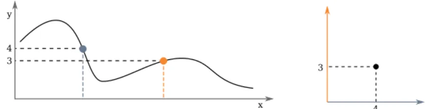
sum of the individuals being processed (in blue and orange); a random tree (in yellow) is used to weight each of the indi-viduals to yield a semantic which is geometrically bounded in the sub-region of the semantics of the original trees. . . . 36 2.4.1 Mapping between the problem space (on the left) and the

semantic space (on the right). Note how the dimension of the semantic space is defined by the size of the dataset (2, in this case), and not by the dimension of the problem input space (1, in this case). . . 39

(8)

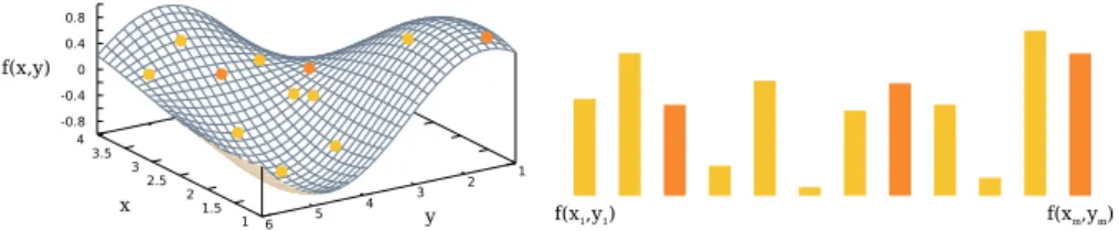
2.4.2 A representation of the semantic of a function f(x, y). The function is usually unknown (thus, it is the objective), but a number of samples are given, therefore we know the val-ues assumed by the function for a given set of input valval-ues, (xǉ, yǉ), (xǊ, yǊ), . . . , (xm, ym). The set of known values is

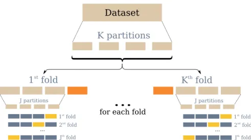
the semantic of f. The number of samples is crucial to being able to capture, and therefore to approximate, the unknown function (compare orange and yellow samples). . . 40 3.1.1 To train the models and then select them, the data should be

split in 3 partitions: training, validation and testing. We use nested K-fold cross validation. In this representation, data that is used for training is represented in blue, data that is used to validate the models is in yellow and test data to evalu-ate the overall performances is colored in orange. Each block is a partition p of the data and folds are union of different par-titions. . . 48 4.3.1 Fitness value of the best individual in the population at each

generation for the bioav train dataset. These values are av-eraged for all the 60 runs performed, and reports both the median value that the median absolute dispersion for each curve. In this case, UGP appears to be the best performing algorithm. . . 65 4.3.2 Fitness value for the best individual in the population for the

bioav test dataset. The curves represent the median values of the 60 runs and to each curve is associated its median abso-lute dispersion. From this plot, we can see that UGP is likely overfitting, while UGPS is performing very well since the be-ginning of the evolution. . . 65 4.3.3 These histograms represent the absolute frequencies of the

fitness values of the best individuals of the population over the 60 runs performed, for the test bioav dataset. As visible, GSGP suffers from a few outliers, but overall has a good final performance which is comparable to UGPS. . . 65

(9)

4.3.4 These plots represent the Euclidean distance, as evolution proceeds, between the semantic of the best individual at gen-eration 0 with the semantic of the best individual in each other generation. The topmost plot shows the semantic dis-tances for train and test datasets when GSGP is run, while the bottom plot shows the same for the UGPS algorithm. Semantic evolution for UGP is a flat line, due to overfitting, and was not reported. . . 68 4.3.5 These plots shows the contribution of the models that took

part into evolution. In the top one, the contribution is shown for each selected model during the evolution, while below it is shown the histogram of contributions at the last genera-tion. These plots refers to models used by UGPS. In the case of UGP, the only contribution was brought by Decision Trees. 69 4.3.6 This pie chart shows the average running time for the UGPS

algorithm. The light gray represents the time required to per-form the selection of models, while the remaining part is rel-ative to the long run. These times are averaged for the 60 runs, and it is visible that the strategy we adopted to select the models is clearly requiring a major computational effort. This is due not only to the number of models, but also to the fact that each model was run 20 times in total, due to nested folding cross validation. . . 70 4.3.7 These plots show the distribution of fitness values for the

three algorithms, both for train (above) and test (below) datasets. The represented median values are paired with median ab-solute dispersion of the data. As it happened with the bioav dataset, we can witness again to an overfitting phenomena. . 71 4.3.8 Above: the contribution, during the evolution of the UGP

algorithm, of all the models. Below, the same plot, but for UGPS. Note how in UGP the contribution values are much less noisy than the ones in UGPS. We attribute this fact to Decision Trees being an overfitting solution which has been discarded by the selection procedure in UGPS. . . 72

(10)

4.3.9 This histogram shows that some combination of models were selected more frequently by PESP, but note there is not a prevalent group. Interestingly, Decision Trees are never se-lected, but Random Forest are always sese-lected, suggesting that the former might lead to overfitting solutions. . . 73 4.3.10This figure shows evolution of semantic distance between

the best individuals. Note that there is a progress in the evo-lution of the semantic, even if the initial soevo-lution turned out to be very good since the inception. We attribute this fact to the ability of GSGP to escape local optima and improve the solutions. . . 73 4.3.11In these plots, we can see how UGP and UGPS perform against

GSGP in terms of fitness values of the best individuals dur-ing the evolution. The new algorithms are performdur-ing very well on training data, scoring almost zero error, and are still significantly better than GSGP on the test dataset. . . 75 4.3.12Above, the plot shows the evolution of the fitness values of

the best individuals when using UGP. Below, the same plot for UGPS. Note how the train and test values are stable, with-out increasing or decreasing over time. This likely means that the Base Learners found an optimal solution and that GSGP is not able to improve upon it, not even by overfitting. 76 4.3.13In this figure, plots of distance evolution of GSGP (above)

and UGPS (below) are compared. Note how, while GSGP is actually working on the transformation of semantic values over the evolution, UGPS has never changed the semantic of the best individual. This is likely due to the elitism mecha-nism, which kept a solution from a basic learner into its place, with no chances to alter it. This is due to the fact that such solution is an excellent result, possibly not far from being a global optima. . . 77

(11)

4.3.14These plots show fitness values of the best individuals during the evolution. As visible in the plot above, the fitness value in UGP and UGPS is almost zero, meaning that the algorithm can model the training data almost with no errors. Below, we can see that the error on test data is not zero, as expected, but it is not a case of overfitness, as the algorithms are per-forming much better than GSGP, even if evolution did not bring any significant contribution in the final results. . . 79 4.3.15In this plot it is visible the evolution of the semantic distance

between the best individuals at each generation since the first generation. Note how, both in UGP and UGPS, above and below, respectively, evolution could slowly change the se-mantics. This appears to be a case in which GSGP escaped a local optima and could find another area to exploit in the fitness landscape. Interesting to note how the semantic dis-tance, albeit on a very small scale, has its major shift in the test dataset only. . . 80 4.3.16This plot shows the contribution brought by selected models

during UGPS evolution. Note how Genetic Programming and Decision Trees are the main contributions, strictly tied to each other. Random Forest scores also a relevant contri-bution during the evolution. . . 81 4.3.17This histogram shows the average relative contribution of each

model at the last generation of UGP. In this case, we can see that Decision Trees and Genetic Programming are con-tributing almost exclusively to the evolution, altgough Ran-dom Forest has also a minor role in this process, influencing about 7% of the final best solution. . . 82

(12)

1

Introduction

In this chapter we will see what are the motivations of this work and which problems it tries to solve. We will overview the concepts and the ideas that are involved.

1.1 Learning Machines to Solve Hard Problems

Some tasks are very easy for humans

As humans, we daily face a high number of problems which are not clearly defined and for which the process that involves the identification of a solution is very hard to define. For some of these problems we have a natural talent and we can solve them quickly and effortlessly: recognizing a friend in a crowded place, walking to her without bumping in other moving people, talking and hearing her voice over the noise of other people chatting and, of course, un-derstanding what she says and having a decent conversation are tasks which we can solve without even realizing how complex they are. Although we might be (partially) hard-wired to solve this kind of problems (for example, a baby can learn any language independently from which language and the baby’s

(13)

origins[82]), we are not born with the knowledge to solve these problems, and we develop the required skill naturally, in our infancy.

Tasks easy for humans might be very hard to formalize and resolve algorithmically

Programming a computer to solve the problems listed above is an extremely difficult task with current technologies, mostly because the problems are not precisely defined on multiple levels: the task of “identifying a specific friend in a crowd” might be easy to understand or formulate, but an in-depth spec-ification of how such a task can be carried is very hard to define. A typical individual can indeed recognize a friend in a crowd, but is absolutely unable to explain how he can do that: it just happens and the inner working, that is, how the brain works, is still mostly a mystery, a black box.

Machine Learning is a way to solve hard tasks with experience

Machine Learning (from now on, ML) is one possible attempt to solve this kind of problems automatically using computers. Mimicking humans, the idea behind ML is to learn from data and experience: observe data to extract interesting patterns, summarize knowledge and devise an automatic proce-dure that can use that knowledge to solve specific tasks. To state it more rig-orously, with the words of Tom Mitchell[70]:

A computer program is said to learn from experience E with re-spect to some class of task T and performance P, if its perfor-mance at tasks in T, as measured by P, improves with experience E.

Typical learning tasks are supervised, unsupervised or by reinforcement

The learning process is usually iterative and can be formulated in different ways: do we have a teacher or not? Can we perform actions in the environ-ment, or not? Do we know the correct answers to the questions we might have on the problem or shall we figure them out by ourselves? Is the environment deterministic or stochastic? Depending on the answer to some of these ques-tions, we can group ML techniques in different categories. One diffused cat-egorization divides approaches in 3 groups: supervised learning, in which we are given a set of observations, a question on these observations and a correct answer to every of these questions; unsupervised learning, in which we are given observations and a question, but no knowledge regarding the answer; reinforcement learning, in which we can act in an environment, collect obser-vations following our actions and in which a teacher may, from time to time, provide feedback to our behavior toward a given objective. More formally, in

(14)

supervised learning, we are given a dataset of examples comprising both input to the program and the expected output,D = {(xi, yi)}Ni=ǉ, where N is the size of the dataset (number of examples), xiis the i-th input and yiis the i-th out-put (also known as response variable and label). If the outout-put is continuous or from an infinite set, for instance yi ∈ R, we talk about regression problems, otherwise, when it is discrete, categorical or nominal, we talk about classifi-cation problems[73]. In the case of learning from data which is not labeled, the task is usually to learn a description of the data. In this case, we talk about unsupervised learning or knowledge discovery, and we haveD = {xi}Ni=ǉ. Fi-nally, when we are given partial information in response to our actions, we talk about reinforcement learning, in which the objective is usually to learn a be-havior, or a policy, that guides our actions inside an environment[95]. In this thesis, we deal exclusively with solving regression problems in a supervised learning context.

The concept of machines able to learn is as old as computers themselves

Being learning a fundamental activity in all human individuals and our so-ciety, it is not surprising that the idea of machines that could learn is rather old in the history of computer science. In fact, Alan Turing himself hypothesized the idea of Machine Learning:

If the machine were able in some way to ‘learn by experience’ it would be much more impressive. If this were the case there seems to be no real reason why one should not start from a com-paratively simple machine, and, by subjecting it to a suitable range if ‘experience’ transform it into one which was much more elab-orate, and was able to deal with a far greater range of contingencies[98]. The concepts that he formulated are fundamental in the ML community: it is in fact important that not only a machine is capable of learning, but it is also able to apply its knowledge in a wider set of situations. When this happens, we say that the machine is able to generalize.

First machine learning models to solve games or model the brain

Since him, pioneers devised a variety of ways to let machines learn, for in-stance by using statistical or probabilistic techniques to infer parameters of a model, or by producing computer programs which can write computer pro-grams. Arthur Samuel pioneered the field by coining the term Machine Learn-ing and explorLearn-ing the application of learnLearn-ing problems by developLearn-ing a pro-gram that played checkers and improved its performances after playing against

(15)

itself[90]. Other pioneering approaches include, for example, the work of Mc-Culloch and Pitt who, in 1943, introduced a computational model of the neu-ron, a single cell of the brain[64]. This funding work opened the path to the field of research later known as connectionism.

Natural evolution was a source of inspiration for solving computational problems

More relevant to this thesis are the works in the field of Evolutionary Com-putation. The idea can be traced back to Turing who, in 1948, proposed the use of genetic or evolutionary search, with genes combination and survival as goodness measure[97]. It took more than a decade to have advancements on this front and, during a short time-span in the 1960s, different research groups come up with approached inspired to natural evolution. Evolutionary Pro-gramming, Evolution Strategies, and Genetic Algorithms were introduced[29,

37,86], opening the path to new research fields. In the last decade of the 20th century, a new research field born, namely Genetic Programming[44,45], and all of them converged in the field of Evolutionary Computation.

Individuals that are fitter in an environment survive and reproduce more

As evident from their names, the underlying principle is to borrow the prin-ciples of Darwinian evolutionary theory to solve problems. In this theory, individuals compete in a given environment with a limited set of resources. The individual that fits best in its environment (which is not necessarily the strongest or the fastest) will survive more, therefore will have more chances to reproduce and to generate more offspring. Newborn individuals are subject to small random changes from their parents that will, over time and thanks to the selection mechanism, lead in significant shifts in how the individuals com-pete and are fit in their environment[23]. The environment is very important to determine how individuals will evolve: the fitness of one individual is not one intrinsic property, but is something defined with respect to it. The dif-ferentiation among individuals is due to the differences in their genetic code, or genotype, which in nature is a long and complex protein that determines the physical appearance of the individual and its abilities to interact with the environment and other individuals, this is called the phenotype.

Evolutionary Computation is based on a loop of evaluation and modification of

individuals

Each evolutionary algorithm is based on different ideas and interpretation of these principles, but the fundamental idea is that individuals can represent a solution in an optimization problem to be solved and that evolution is a mean by which solutions are modified until they are satisfying. Using evolution to solve this kind of problems usually requires defining what a solution is, how

(16)

to represent it and how to measure its fitness, that is, its performances when compared to other individuals.

A motivation for using EC is that evolution is effective

The adoption of an evolutionary approach to solving problems is justified by the fact that evolution is the recognized principle that allowed the existence of humans and a plethora of living beings that are extremely efficient and com-petitive in their environments. It is a very general method that allows to freely adopt any appropriate representation for a given problem and it is often sur-prising in its ability to find unexpected and effective solutions [46,54].

Evolutionary Computation can be used in Machine Learning as well

Evolutionary Computation involves an iterative process that produces, by successive refinements, a solution to a problem that is hopefully acceptable. ML and optimization techniques are strictly interconnected: to find a model which is able to generalize it is necessary to solve an optimization problem, for instance that minimizes a given error over known data. The ability to general-ize, and therefore having a model which really has “learned” the essence of the problem under some sense, usually requires additional steps and care. There-fore, Evolutionary Computation can be used to solve problems using ML, and with time and experience we can see that it is also a quite effective technique.

Machine Learning has a major role in our current lives

In the years, Machine Learning acquired a major role in the tools we build and use in our daily lives, and it is very hard for an individual in our society to not using it, directly or indirectly. For example, automatic learning is used in manufacturing, in production, dispatch or selling of goods and, of course, in the service industry.

There are many ML models and making a choice is not always easy

The role of ML is especially of particular importance for every person that has to make sense of (many) data, and the scientific community is not ex-cluded. Indeed, the level of literacy regarding coding and software develop-ment is increasing in the years, and so it is the knowledge regarding ML. Nowa-days it is very common to run algorithms that learn from data to perform basic tasks such as regression, classification, and clustering: it often gives insights on the data and improves the quality of the results for the entire scientific com-munity. Nevertheless, the pace of progress in the ML community and the number of models available is overwhelming and a regular scientist does not always have time to learn properly how each algorithm works, how to use and how to tune it. Therefore, it is not surprising that a small number of simple (to use and to understand) algorithms are being widely used for a multitude

(17)

of tasks. These algorithms have the merit of performing well in general, to be conceptually easy to understand and, therefore, to debug and use.

Determining what model to use for a problem is a problem itself

This, however, limits the progress of the entire community. Naturally, an important piece of the puzzle is the role of software engineers and data scien-tists that can abstract from the “low level” of some algorithms and make them freely accessible to the general scientific community, but often this requires careful engineering and design of tools. This effort, although very useful in general, does not eliminate the need of searching for better models: the gen-eral methods will not work in every case, and some other approaches might be more suitable to solve a given problem. Typically, a scientist will evaluate the performances of different ML algorithms over the same problem and use the one that appears to work best.

In his book “The Master Algorithm”, Pedro Domingos discusses an algo-rithm that is capable of solving a plethora of different problems[25]. The research community is working hard towards that goal, but it is still far. He highlights how few algorithms are currently used in a very large variety of ap-plications: the key is naturally their generalization abilities, not necessarily as Machine Learning models, but also as useful algorithms with widespread applications. Evolutionary Algorithms are, in fact, one of the selected candi-dates to become master algorithm: they are indeed very powerful and generic enough to be run many different applications. But, even if they can be applied to many different domains, careful setup and tuning is required to obtain sig-nificant performances and qualitative output. An unifying, higher level algo-rithm is still required to make these powerful algoalgo-rithms more usable.

Many paths are being explored in the attempt to automatically use the best model

Numerous approaches are being explored, included but not limited to trans-fer learning, ensemble methods, hyper-heuristics, and meta-learning. The for-mer is the practice of learning from one experience and transfer the experi-ence to solve new problems. This practice is diffused in the connectionism field. Ensemble methods, on the other hand, try to solve a problem by using a number of models, similar or different among themselves, and selecting or combining them to yield performances which are better than the constituting parts. Also hyper-heuristics and meta-learning, which have many similarities among them, try to solve a problem by employing a multi-tier approach in which one algorithm tunes or builds one or more algorithms to solve a given

(18)

problem. These methods work by working on a more abstract level, for exam-ple by selecting which underlying algorithm to use for a given problem or by tuning the (hyper) parameters of the underlying algorithm. We will discuss these approaches in the next section.

We think a middle-level abstract could help in automating this task

What we think is still missing to these approaches is the presence of a con-ceptual middle level which creates an abstraction layer: while it is true that we can combine multiple models in an ensemble method, it is also true that how we combine them greatly depends on what kind of models they are. The same can be said for hyper-heuristics and meta-learning: although it is indeed possible to use an algorithm to tune the parameters of another algorithm, the former must be designed so that it knows how to work with those parameters and this requires a knowledge of the algorithm itself. This approach can be very useful and achieve great results, but it is not universal.

1.2 Objective of this work

Our objective: build an ensembling algorithm using an intermediate representation

For the reasons introduced above, in this thesis, we tackle the problem of building an unifying algorithm which uses an “intermediate representation” to abstract from the model actually used and, therefore, is extremely general. We will see how recent advancements in the field of Genetic Programming en-abled a new way of searching for problem solutions and how this might impact the Machine Learning community in general.

Geometry Semantic Genetic Programming is a good starting point thanks to how it uses semantic

In particular, we will build upon the results obtained by the Geometric Se-mantic Genetic Programming community, in which the concept of seSe-mantic is key to build the necessary abstraction. In this context, the semantics of a program has the same meaning of the image of a function in mathematics: given a set of input data, the semantic of a program is the value of that pro-gram on each of those data. However, we will usually deal with data in tabular form, therefore the semantics of a program will be a vector instead of a set.

Semantic can be a valid intermediate representation for any ML model

We will see how this approach is flexible in the sense that it can be used with any underlying model, as long as the output of such a model is meaningful. We will discuss the principles and the algorithms in detail, showing how the algo-rithm we are introducing will have to face the same problems that are to be faced by Machine Learning practitioners when they look for a given model.

(19)

We will suggest a solution to these problems and provide an implementation of the algorithms. Then, we will test these implementations on five different datasets, comparing the obtained results with the results obtained in the liter-ature.

1.3 Structure of this work

This thesis is structured as follows. In Chapter 2 we provide the necessary elements required to contextualize and understand this work; in it, we will in-troduce the concepts of Genetic Programming, Geometric Semantic Genetic Programming and Ensemble Methods, seeing how the current state of the art could be advanced to exploit even more the concept of semantic. In Chap-ter 3, we will introduce the main contribution of this work: two variations of Geometric Semantic Genetic Programming called Universal Genetic Pro-gramming with and without pre-evolutionary selection. In Chapter 4 we will show the tests performed over five datasets to support the utility of the algo-rithms and discuss their results. Finally, in Chapter 5 we will discuss the out-come, the flaws and the qualities of the proposed algorithms and the obtained results, suggesting possible improvements and new paths for future research.

(20)

2

Background

In this chapter we lay out the foundations over which this thesis is developed. We will introduce Evolutionary Computation and Genetic Programming. We will introduce the concept of semantic of a program and introduce Geometric Semantic Genetic Programming, which is built upon Genetic Programming and onto which we will build upon. We will also introduce three classes of methods that try to improve our efficiency in using Machine Learning mod-els by combining and tuning them automatically. These are Ensemble, Hyper Heuristics and Meta Learning methods. They are similar in their intents, but each one presents some key differences from the others that we will introduce.

2.1 Evolutionary Computation and Genetic Programming

GP is an algorithm that is able to create programs using evolution

Genetic Programming (from now on, GP) is an active and exciting research sub-field of Evolutionary Computation [27]. The main characteristic of GP is that it can be used to solve optimization problems by producing computer programs through the principles of natural evolution. In particular, GP uses

(21)

an iterative process which involves refining randomly generated programs by selecting, reproducing, combining and modifying them until the desired level of approximation is reached on the problem to be solved.

GP is a very flexible optimization algorithm with multiple application domains

GP has been used to solve a variety of problems, for example to generate art [22,59,88], to design satellite antennas [56], to play chess [36], in game theory [20], to develop RoboCup players [58], for forecasting of complex phenomena (crime rates [19] or ozone concentration [17]), quantum com-puting [94], symbolic regression [11,44], sorting[41], signal processing [61] and in many tasks it performed very well, producing human-competitive results[46].

We will now review the fundamental concepts in GP, but for a more broad overview we suggest [5,44,45,53,83]. We will start to analyze GP from a specific case, known as Standard GP [44].

Optimization problems as search in a solution spaceS

To set up an effective evolutionary process that finds solutions to a problem, it is first necessary to formalize and set a representation for the solutions to such a problem. In general, given a setS ofsolutions, anoptimizationproblem consists in finding one or more s ∈ S such that they satisfy some desirable properties. To quantify how much a solution is desirable, a function f :S 7→ R is usually employed to measure the performances of such solutions. If a better solution has a higher value of f, the problem is said to be a maximization problem, otherwise it is a minimization problem.

Different representations might impact the efficiency of the search

How solutions inS are represented is fundamental to solve efficiently a problem [76,89]. For example, given an instance of the classic Traveling Sales-person Problem (TSP), in which the input is a graph describing the distances between the places to visit, a solution could be represented as a sequence of places to visit, with no repetitions, or as a program written in C that reads the graph as input and computes the length of the shortest path. In the first case, the space of solutionsS corresponds to the set of permutations of the cities, and evaluating a solution is done by summing the distance between subse-quent pairs of cities (that is, f contains the knowledge necessary to interpret the sequence and to produce an output value), but in the second case,S is the set of programs that can read the graph and return a valid real number, which is a much larger space (consider, for example, that there are multiple algorithms that can be used to solve the same problem). As can be seen, while the first representation looks naturally efficient to solve the TSP problem (although,

(22)

we are not stating that it is the most efficient representation), the latter could be suitable to solve a class of problems as it can process any graph. This difference is what makes GP different from other evolution algorithms such as Genetic Algorithms (GA), in which the representation of a solution shall be, at least in its original formulation, a linear sequence of fixed length. Since in GP there is no such restriction, it could be argued that GP is a class of algorithms that include Genetic Algorithms as well [49].

How solution are represented heavily influences our ability to search inS

Even if the space of solutionsS is not the only factor influencing the dif-ficulty of solving a problem with GP, in practical terms, it is often a primary concern and for this reason the selection of a representation is crucial for solv-ing a problem [30]. In the following discussion, we will see how the structure of f andS has a role in the difficulty of a problem. Selecting a representation is very important, not only by impacting the search efficiency, but determining if an optimal solution can be found at all.

Standard GP uses trees to represent usual arithmetic expressions

In Standard GP, solutions are often represented as arithmetic expressions composed by the usual operators: addition, subtraction, multiplication and division, defined on real numbers. To efficiently represent these expressions, operators are combined into a tree, in which internal nodes are the operands and leaves are scalars. Those scalars can be numerical constants, such as π or ǌǊ, or input variables, such as xǈor xǉǊ, with xibeing the i-th component of a

given input vector x

Many different

representations have been used in literature

Although GP imposes very few constraints on the kind of solutions it can work with, we will deal mostly with solutions represented as trees, as we just described, hence we will discuss them in detail. Nevertheless, it is not re-quired to adopt expression trees, and many other representations have been used successfully including, for instance, lists [7], assembly languages [21], stacks [80,93], grammars [75] or binary space partitions [84].

Terminals are leaves of the tree, internal nodes are functionals with various arity

In the context of Standard GP, as well as in our case, trees are composed by nodes which are either functionals or terminals. Functional nodes are nodes that accept inputs and produce a single output, while terminals are nodes that accept no inputs. Functionals with a single input, such as the absolute value function|·|, are said to be unary. On the other hand, functionals with two in-puts, such as the sum function·+·, are said to be binary operators. In general, the arity of one operator determines how many inputs it accepts. Terminal

(23)

nodes are either constants, variables or nullary operators, while functionals have arity greater than zero.

Programs can use one or many data types in a weakly or strongly typed fashion

Until now, we assumed that functionals and terminals were real-valued, but it is not necessarily so: the definition of different types is an important topic in computer science, and GP is no exception. Although strongly, multi-typed GP systems exist [71], in which it is possible that multiple data types coexist in the same evolutionary process. In our case we impose that every node in the tree assumes a value of a single type, that is a real number, as it is com-mon when defining usual arithmetic expressions. Therefore, our functionals are closed under their type, meaning that they accept parameters of the same type they assume. to keep the individuals in a consistent state. Note that the tree structure imposes a precedence on the operators, as it is usually evaluated recursively from leaves to its root, therefore it is not necessary to have paren-theses.

Error handling is an important part of automatic program production

It is also important to define how errors and exceptions are handled. For example, the division operator is usually not defined over zero and trying to perform a zero division will likely cause a runtime error in the system where GP is programmed. Similar argument can be made for any function with lim-ited domain: for example, logarithms cannot have negative argument. There-fore, to avoid errors, specific functions are defined (for example, the division operator will be defined in 0, for example by assuming value 1), or constraints on data are imposed, so that it is possible to compute an expression without compromising the overall evolution.

To increase the effectiveness of a GP system, Koza suggested to select func-tionals which are closed, that is, they are both type consistent and safe to eval-uate [44].

The evolutionary process acts upon a population of individuals (solution)

Once a representation has been set, the evolutionary process begins by con-sidering a set, usually constant in size, of solutions. Borrowing from biology, solutions are often named individuals and the set of individuals is called pop-ulation. Such a set is initialized by an initialization operator, which adopt a certain initialization strategy to define which individuals will compose the ini-tial population. In Standard GP, where trees are used to represent expressions, there are three common ways to initialize individuals: grow strategy, full strat-egy and ramped half-and-half.

(24)

Trees are built with different strategies such as, grow, full and ramped half-and-half

The grow strategy consist in picking a random node among the entire set of functionals and terminals: if a functional is selected, it is used as a root, and the grow strategy is applied recursively to create each of its nodes. The procedure ends when a terminal node or a maximum depth is reached: in this latter case, selection over terminal nodes is enforced at the maximum height. In the full strategy, full trees are created by randomly picking functional nodes until the last but one level is reached, at that point, only terminal nodes can be selected as leaves. In the ramped half-and-half, both grow and full strategies are used to initialize half of the population each, with the constraint that instead of using a single maximum length, a range of heights is used so that different fractions of the population will be initialized using a different maximum height. This ensures a higher degree of diversity within the initialized population. Ramped half-and-half is a widely used initialization strategy and we will use it in this work as well.

GP uses an iterative process to evolve the population

Before the iterative process begins, the initialization operator will create individuals according to the selected strategy. In the context of Standard GP, every individual is initialized accordingly the chosen strategy, yielding a popu-lation of randomly generated trees (expressions). Once initialization has been performed, the iterative evolutionary process will start. Every iteration of this loop will be referred as generation, and as it happens with natural evolution, each generation of individuals is the result of natural selection applied to the previous generation.

Selection, reproduction, recombination and mutation are the basic operators in GP

In nature, during a generation, individuals are first selected, then they can reproduce and usually some amount of recombination and mutation will hap-pen to their DNA, via sexuated reproduction and environmental influence. In GP, this process is performed by the selection, crossover and mutation oper-ators. Selection operators require that the performances of each individual have been computed: each individual is, in fact, a solution of the optimiza-tion problem we are trying to solve and after evaluating it (e.g. by compiling and running it) over the problem inputs, we can measure the quality of the outputs and determine its fitness, that is, how fit the individual is in its envi-ronment and how likely it is to reproduce. The higher the fitness, the likely one individual will reproduce.

The fitness function determines the goodness of each individual

Generally speaking, the fitness of one individual is a quantity that we want

(25)

to maximize: more fit means a better individual in its environment. In the field of Evolutionary Computation, the meaning of fitness can often be dif-ferent from the biological term, and fitness function is often interpreted as an objective function, that is, f. Therefore, for maximization problems, the ob-jective is to search solutions s ∈ S that yield the highest value in f, while for minimization problems, we seek solutions that yield the lowest possible value of the fitness function. We will adopt this convention where fitness function and objective function are the same entity, and we will restrain from referring to a specific minimization or maximization problem by speaking, more gener-ally, to a better or worse fitness value. In minimization problems, better means smaller, while it means larger in maximization problems.

Selection operators use fitness to determine which

individuals will survive one generation

The fitness of each individual is therefore used by the selection operator, which randomly picks every individual with a probability that is correlated to its fitness. In other words, the better the fitness, the higher the probabil-ity an individual will be selected. As with initialization, there are different strategies to select individuals. Common strategies are Tournament Selec-tion [6,68] and Proportional Selection [31]. In the Tournament Selection, a fixed number of individuals (the tournament size) is randomly selected with uniform distribution and, only among those individuals, the fittest individual is selected as tournament winner and it can, therefore, advance from one gen-eration to the next (i.e. survives the natural selection). Another widely used strategy is the proportional Selection, also known as Roulette Wheel selec-tion, in which each individual has a probability to be selected for reproduc-tion with probability proporreproduc-tional to its fitness. Note how, in this case, fitness must be computed for every individual, while it is this does not happen for the Tournament Selection.

Selection pressure reveals how much individuals are

competitive in surviving

A property of selection strategies is their selection pressure, which is a mea-sure of how the system is biased towards fitter individuals: if the selection pressure is high, individuals with better fitness will have a much higher prob-ability of being selected, while if selection pressure is low, all individuals are likely to be selected independently from their fitness. For example, if the tour-nament size is equal to 1, selection pressure for the Tourtour-nament Selection is at its minimum and every individual will be selected with uniform probabil-ity (any selected individual is also the winner of its tournament), while if the

(26)

tournament size is large, only the fittest individual will be selected, therefore the fittest individuals in the population will likely survive. It is obvious that, if the population size is constant from one generation to the next, selection is meaningful only if individuals are selected with replacement, otherwise all individuals would be selected and survive each generation. The ability of one individual to be selected multiple times, roughly correspond to the ability of a living being to reproduce more. We illustrated tournament selection as it is the strategy we are using in this work, but many more selection schemes that have been studied and adopted in literature. For a more in-depth analysis, the interested reader can refer to [31,63,67].

Crossover swaps genetic material, while mutation introduces genetic novelty

Once selection is completed, individuals might be present in multiple copies and are therefore reproduced. To these individuals are then applied the re-combination and mutation operators [57,102]. Recombination operator, of-ten called crossover, intuitively works by swapping genetic material between two individuals. More precisely, it combines the representations of two or more ”parent” individuals to produce one or more ”children” individuals that are built with fragments of the parents. Note that no new genetic material is introduced, but the existing material is recombined. In the context of Stan-dard GP, two parents can be crossed over to produce two children by ran-domly swapping elements from one parent to the other. There are, as usual, multiple strategies for doing this, but the one most adopted is to swap two random subtrees, which can be selected completely randomly, or with some constraints (e.g. never pick root nodes, or pick random subtrees so that, af-ter swapping, the resulting trees do not exceed a maximum height limit). On the other hand, mutation, which is represented along with crossover in Fig-ure 2.1.1, is the operator that introduces new genetic material. Mutation is fundamental to explore the entire solution space, because with its absence, the available genetic material would be determined at initialization (e.g. if no expression with a sum is generated, then no expression can have a sum in it, which might be fundamental to reach optimal solutions). Mutation works on a single individual and changes it in a random fashion and, as with every other operator, there are plenty of strategies that can be applied. A common strat-egy, when working with trees in Standard GP, is the Subtree Mutation, which consists in randomly picking a node in a tree and replacing it with a randomly

(27)

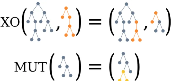
Figure 2.1.1: A representation of crossover (XO) and mutation (MUT) operators in Genetic Programming. The crossover operator is often imple-mented as an operator that swaps two random subtrees of the individuals being processed (in blue and orange); this yields two children, which often take the place of the parents in the population, but some implementation use just one of these two. The mutation operator is often implemented by replacing a random subtree of the individual being processed with a subtree that has been randomly generated (in yellow).

generated subtree (possibly limiting the height of the generated tree, to satisfy height constraints for the resulting tree). Another common mutation is Point Mutation, which randomly picks a node in the tree and replaces it with a ran-dom node with the same arity (i.e. a terminal with a terminal, or a functional with a functional with the same number of arguments) [83].

The iterative process continues until a termination condition is met, for ex-ample, the evolution stops after a fixed number of generations, or when the fitness of the best individual in the population reaches a fixed threshold. A representation of the algorithm is shown in Figure 2.1.2.

Elitism preserves the best individual from one generation to the next

It can be seen from this explanation that there is no guarantee that a good solution, once found, survives the selection mechanism. In fact, we are usu-ally interested in finding the best possible solution encountered in the entire evolution process, not the best one at the last generation. Elitism is a strat-egy used by GP to guarantee that the best individual will survive the selection process. Usually it means that the fittest individual is automatically included in the population of the next generation, without undergoing any selection procedure. This means, of course, that the fitness must be evaluated for every individual at every iteration, but employing elitism is often a good strategy as it helps to improve the overall fitness of the population.

(28)

Figure 2.1.2: A representation of how the evolutionary process works. After initializing the population, the main loop begins with the selection of which individuals that will survive; then, those individuals will be mod-ified by genetic operators (primarily mutation and crossover). The result-ing individuals produce a new population that will replace the initial one, and the loop will then continue with the next iteration (generation).

(29)

The concept of neighborhood provides a structure over the space of solution

Useful when reasoning on GP are the concepts of neighborhood and of fit-ness landscape. The neighborhood of one individual is the set of solutions that can be obtained by transforming it according to one application of recombi-nation or mutation operators. If the fitness of an individual is better than the fitness of all its neighbors, then the individual is a local optimum. A global op-timum is the best individual among all local optima. Note that multiple global optima might exist, but their fitness value will be the same.

The structure of the neighborhood defines the fitness landscape of the problem

The concept of fitness landscape is based on the idea of neighborhood, but gives an insight on the difficulty of a problem by mapping the structure of the individuals and their neighborhood in a geometric space [76]. There are different definitions, all roughly equivalent, of fitness landscape, but in sim-ple terms, it is a plot where solutions are placed on the horizontal direction (as independent variables) and their fitness is placed on the vertical direc-tion (as dependent variable) [52]. If the solutions can be represented in a 2-dimensional space, consistently placing the neighborhood structure on the axis, the fitness landscape can be seen as a 3-dimensional map where tops of hills represent local optima.

Fitness landscape as a 2D graph in which nodes are sorted along one axis according to their fitness

Another view of the fitness landscape, alternative to the continuous ”map”, can be obtained by drawing a graph in which solutions are nodes and the neighborhood relationship is represented by edges. This graph places nodes sorted vertically according to their fitness, with nodes with the same fitness on the same level. Local optima are nodes whose adjacent vertices are positioned in lower levels. The topmost nodes are the global optima. This representation has the advantage of not requiring to sort solution on multiple axes accord-ing to their neighborhood structure, which translates to an easier visualization which does not require to place solutions in a high dimensional space. A sim-plified representation of some fitness landscapes can be seen in Figure 2.1.3

The difficulty of a problem is sensibly influenced by the fitness landscape

From the fitness landscape it is possible to understand the difficulty of the problem by considering how many local optima there are [42,69]. Simpli-fying, the less local optima, the better, and the less plateaus, the better. To understand this intuitively, consider picking a valid, random solution. If the solution is a local optimum, it means that none of its neighbors are better than it, therefore no mutation or crossover is sufficient to find a better solution in a single step. Naturally, since the selection mechanism is stochastic, it is

(30)

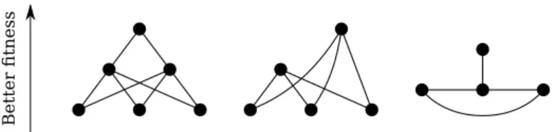
possi-Figure 2.1.3: In this scheme are represented three, very simple, fitness landscapes. Each node represents a solution, which are sorted on the y axis depending on their fitness value. In the leftmost graph, we can ob-serve that there is only one local optima, the topmost node, therefore it is unimodal. In this case, there are no plateaus, because each node can have only neighbors with better or worse fitness. In the central landscape we can observe two local optima, but only one of them is also a global optima. This landscape is therefore not unimodal. On the rightmost fig-ure, we can see that the landscape is unimodal as there is only one local optima, but a space with a similar structure might not be easy to search as it is easily possible to jump among bottom nodes without finding the best one.

ble to escape a local optimum if the peer pressure is not excessively high. On the other hand, if a single global optimum is present and if every solution, but the local optimum, has at least one better solution, it is easier to find the global optimum, as the likelihood of improving is much higher due to the fact that from every solution it is not required to backtrack to worse fitting solutions to reach a better one. A landscape in which there is only one local optimum is called unimodal, otherwise it is called multimodal.

Unimodal fitness landscapes are often desirable

As we explained, having a unimodal fitness landscape is usually a desirable property, but not every fitness landscape that is unimodal is easy to search. As an example, consider a fitness solution which assumes value 1 when a specific solution is found and 0 in every other point. The associated fitness landscape will have a single spike, connected to all its neighbors, and will be a plateau in every other point. In this case, optimization is very hard for many common neighborhood structures.

2.2 Learning to represent data

It is not always possible to encode the modeled phenomena in the fitness therefore we can use a data-driven approach

In the Standard GP that we illustrated earlier it is possible to identify the space of solutions S, composed by all the trees that form valid expressions and

(31)

for which a fitness value is defined. The fitness function f maps points in the solution space to fitness values. How the fitness is defined depends on the na-ture of the problem to be solved, but in general we described it as a function that maps inputs to outputs. Outputs are just a goodness measure for indi-viduals, and do not have to map directly to the problem. Ideally, the fitness function encodes how the solution maps to the problem and then evaluates its performances. For example, if the space of solutions was the space of all possible programs that safely drive a car, the fitness function would measure how safely and how far the program would drive: the more miles driven with no crashes, the more predictable is the behavior by other drivers and the less rules infringed, the better. The fitness function would probably evaluate the solution program by simulating a virtual environment and eventually would compute a value to determine how good is the program in driving. On the other hand, other problems cannot be solved in this way. Consider, for exam-ple, the problem of determining if a molecule is toxic or not to humans: we are currently unable to estimate the effect of a certain amount of such molecule by simulating the entire human body, therefore we have to approximate the estimation even more and use simpler models. We can abstract this process and assume that there is a function that, given the description of the molecule being studied, can determine its toxicity level on the average human body. It is naturally very hard to explicitly define this function, but we could try to ap-proximate its extension by sampling some of its values by actual measures. In other words, we can give a safe amount of this molecule to human subjects and measure the toxic effects. By collecting more data, we can better approxi-mate the behavior of such function. Naturally, this does not solve the problem we had, but now we can try to approximate the function by fitting the known points.

Using collected data to model a problem is a key practice in ML

Many problems cannot be simulated, or are excessively expensive to sim-ulate, therefore this data-driven approach is very diffused. In the field of Ma-chine Learning, the whole class of supervised learning is devoted to trying to model an unknown function which maps known inputs to known outputs, which are often obtained by external human intervention. As an example, consider the famous problem in the context of supervised learning is the hand-writing recognition problem, in which the known data are a set of raster images

(32)

representing handwritten symbols, with the objective of automatically deter-mine what symbol is depicted. This is done using a dataset in which each digit image is labeled. For example, in the very famous MNIST dataset, there is a collection of images of handwritten digits from 0 to 9.

It is worth noting that these problems are often divided into two categories: regression or classification. A regression problem is a problem in which the objective function assumes values in a continuous space, while classification is when outputs assume discrete values. In this thesis, we will deal with re-gression problems.

We organize data in a tabular form representing the mapping of input variables to one output

From now on, we will assume that data is available in a tabular form, in which a datasetD is a non-empty list of samples of an unknown functionˆf : Rn _{7→ R. Each sample is a pair (X,ˆy) where ˆf(X) = ˆy, and such dataset} basically represents all the knowledge we have on the problem to be solved. Our objective is to identify a function f which is as similar as possible to ˆf, given the dataset.

Performances of a model over some data are measured using an error measure like MSE

When searching the approximated function f, we will measure the perfor-mance of a candidate function by evaluating it on the dataset and measure how distant is the result from the expected output. The distance measure may vary, but the ones commonly used are the Mean Square Error (MSE) and Mean Ab-solute Error (MAE), which we will use in this thesis. The MSE is defined as follows: MSE = ǉ N ∑ i∈Q (ti− yi)Ǌ

where yiis the output of a candidate solution on the i− th training case and ti is the target value for that training case. N denotes the number of samples in the training or testing subset, and Q contains the indices of that set. By using the same notation, the definition of the MAE is the following:

MAE = ǉ N ∑ i∈Q ∥ti− yi∥ .

Naturally, a function f may behave well on the dataset points, but misbehave on every other point. In this case, we say the function f is unable to general-ize well, and in particular that the solution is overfitting. A graphical repre-sentation of overfitting and underfitting (i.e., the opposite phenomenon) is

(33)

displayed in Figure 2.2.1.

Figure 2.2.1: Overfitting and underfitting models. A model is said to underfit if it is not complex enough to capture the phenomena to be modeled and, at the opposite, it is said to overfit if it is so complex that learned the data without ability to generalize.

Overfitting and underfitting models often are unable to capture underlying phenomena

Overfitting functions are not often useful: they do not model correctly the problem and cannot be used to predict the behavior of the function ˆf for a given input. The generalization abilities of a solution are very important when solving a problem that requires to sample new points from that solution, there-fore evaluating the generalization performances of a solution is an important task. Naturally, one may evaluate those over new data if they can be acquired: this is what is usually done in a scientific context, where new evidence is used to disprove failing theses. If it is not possible to acquire new data, a possible evaluation process involves using two different partitions (i.e. with empty in-tersection) of the dataset: one partition is used to search for a solution, while another partition is used to evaluate its performances on unseen data. Get-ting rid of overfitGet-ting altogether is not possible in principle, but in this thesis we will cite few methods to reduce the chance of it happening.

(34)

2.3 Geometric Semantic Genetic Programming

When a solution f is evaluated on an input, it yields a point in its codomain,R in our case. Depending on the error measure we selected, that point will have a certain distance from the desired output, which is hopefully (but unlikely) zero.

The semantic of a function f is the values it assumes on the datasetD

Assume now that the samples in the dataset have a fixed order, that is, each sample is numbered from ǉ to m, being m = ∥D∥ the size of the dataset. Then, if we evaluate a solution over the entire dataset, we can build a vector

Y = [yǉ,· · · ym] = [f(xǉ),· · · , f(xm)]

which is called semantic. This m-dimensional vector can be positioned in the Rm _{space of vectors called semantic space, representing the space of points} obtained by evaluating all the possible solutions over the datasetD. The de-sired solution, ˆy is, of course, a point in this space, and the distance between two semantics is the distance between two points of this space, under some metric.

The optimization problem overD can be state in terms of semantics

Adopting this view, the search for ˆf is the search for a solution with a se-mantic that has zero-distance from ˆy. We can now define an equivalent op-timization problem whereSSis the semantic space and ˆfSis a function that measures the distance to the target semantic vector, ˆy. This function will as-sume non-negative values and the global optimum will be in zero, therefore it is a minimization problem.

Any non-optimal semantic has a neighbor which is closer to the optimum

Consider, in this case, the space of neighbors: if we consider an operator that mutates a solution by adding a random noise to any of its components, every solution but the global optimum will have a neighbor with a better fit-ness, because in any position of the space it is possible to identify a slightly different solution which is nearer to the best. We call this mutation box muta-tion, because on every axis of the semantic vector a noise can be added, ideally defining a ”box” around a solution where neighbors are contained. A more rigorous definition of box mutation, with a mutation step μ, is the following:

M(X) = X + Um(−μ, μ)

(35)

where Um(−ǉ, ǉ) is a vector of random numbers distributed in [−ǉ, ǉ] of length m.

This means that such fitness landscape becomes unimodal. As we explained earlier, this is a convenient situation and, although from a given solution it is not possible to determine a better neighbor without knowing the target se-mantic, this situation provides an enormous advantage in the search for a so-lution with respect to the original problem.

We look for operators that work on programs, but transform their semantic as desired

Naturally, solutions in this new problem are not programs: they are seman-tic vectors to which concepts of prediction and generalization do not apply. Semantics are obtained by evaluating a program over the entire dataset and we would like to find a program that is capable of producing such semantics be-cause that program models the originalˆfwe are searching. Therefore we now have to find a way to map solutions from the original spaceS (programs) to the new spaceSS_{(semantics) such that the genetic operators transform} se-mantics as we described by acting on programs.

To perform such transformations on semantics, two semantic operators were introduced [72]: Geometric Semantic Mutation (from now on, GSM) and Geometric Semantic Crossover (from now on, GSC). These two operate on semantics by transforming the generating function by scaling and translat-ing it.

GSM mutates a solution by adding a random noise to the function value

GSM, represented in Figure 2.3.1, operates on a function f : RN 7→ Rm and, in the semantic space, has the effect of a box mutation and is defined as

fM(X) = f(X) + μ· R

where μ is the mutation step, which is a multiplicative factor on how each com-ponent of the semantic will be scaled. Note that, in this case, μ does not im-pose a limit on the possible mutation of each component, therefore we are not actually bounding the box. R is a random vector centered in zero with length m, which effectively allows to apply a perturbation on each component of the original semantic vector. R is usually defined as a difference of two ran-dom trees Tǉ− TǊand sometimes a bounding function is applied to limit the

value of its component in [−ǉ, ǉ], so that the mutation step μ is effectively the size of the ”box” in which mutation happens. Good experimental results

(36)

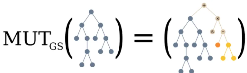
Figure 2.3.1: Geometric Semantic Mutation is represented. In this case, the difference of two random trees (in yellow and orange) is used to per-turb the semantic of the individual being processed.

were obtained with this technique by applying a logistic map over the trees Tǉ, TǊ.[14,32]

GSC combines two solutions into one that has a semantic never worse than its parents

GSC, represented in Figure 2.3.2, works instead by interpolating the seman-tics of the parent individuals. Two parent individuals will have a semantic each that can be positioned in the semantic space as two points. It is possible to identify a single straight segment passing by those points, and all the points on that line can be identified via a single parameter α. Given two points pǉ, pǊ,

all the points on the segment can be defined as p = αpǉ+ (ǉ− α)pǊ

with α∈ [ǈ, ǉ]. This geometric interpretation can be applied to build the GSC operator, which combines two functions fǉ, fǊ : RN 7→ Rmusing a random

scalar value in the way we explained. This crossover has the property that the generated ”child” individual will never have a worse fitness than the worse of the parents. A variant of this operator, used in [14] as well as in this work, uses a vector ¯α with components bound in [ǈ, ǉ] therefore instead of being an interpolation of the two parents, the offspring will be a random point in the m-dimensional box defined by the parents. We have no experimental evidence that this variant is performing differently than the original formulation (the-oretically speaking, this crossover is less effective, as it might introduce worse solutions in the population, but it could also produce a solution which is bet-ter than both parents, which the crossover as defined above cannot produce), and actually it seems that this operator is not useful to evolution [16], but in this work we built upon [14]. Therefore we maintain the same operators to

(37)

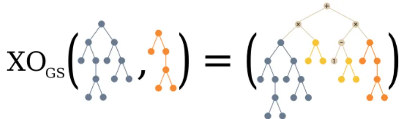
Figure 2.3.2: Geometric Semantic Crossover is represented as the weighted sum of the individuals being processed (in blue and orange); a random tree (in yellow) is used to weight each of the individuals to yield a semantic which is geometrically bounded in the sub-region of the seman-tics of the original trees.

exclude an additional factor that might influence our results, therefore making the evaluation of our algorithms more ambiguous.

GSGP is the GP algorithm that uses the Geometric Semantic Operators

Using these two operators, it is possible to produce a new generation of individuals that not only prevents degradation of performance, but will con-sistently improve the fitness thanks to the geometric properties of the seman-tic space. With Geometric Semanseman-tic Geneseman-tic Programming (from now on, GSGP) we will refer to a Standard GP with a fixed datasetD which maps in-dividuals into a semantic space, computes the fitness as a distance function between individuals’ semantic and the target semantic and uses Geometric Semantic Operators we described.

In GSGP solutions will grow without limits

Without the need for careful inspection, it is evident that these Geometric Semantic Operators combine solutions to improve their fitness, but the com-bination is not destructive. In other words, the size of each individual will grow very quickly due to the fact that each child encapsulates the full defini-tion of its parents. In the field of GP, the tendency of soludefini-tions to grow in size unnecessarily is called bloating [4,24], and often solutions are limited in size. In the case of GSGP, limiting size is not possible, but the quick growth of so-lutions make them hard to handle. Having soso-lutions that continuously grow in size is not a new phenomena in GP: it is referred as bloating and it happens in Standard GP and other setups. Typically, some counter-measures are taken to avoid an undefined growth of the solutions, such as limiting the height of the solution trees so that neither crossover nor mutation will produce any in-dividual with an height greater than the limit. This is naturally not possible