Computational methods for microarray data analysis

(1)

Universidade de Aveiro 2009

Departamento de Electrónica, Telecomunicações e Informática

Bellina Ribau Teixeira

Métodos Computacionais para Análise de Dados de

Microarrays

(2)

(3)

Universidade de Aveiro 2009

Departamento de Electrónica, Telecomunicações e Informática

Bellina Ribau Teixeira

Computational Methods for Microarray Data Analysis

Dissertação apresentada à Universidade de Aveiro para cumprimento dos requisitos necessários à obtenção do grau de Mestre em Engenharia de Computadores e Telemática, realizada sob a orientação científica do Professor Doutor José Luís Guimarães Oliveira, Professor Associado do Departamento de Electrónica, Telecomunicações e Informática da Universidade de Aveiro

(4)

(5)

o júri

presidente Prof. Dra. Maria Beatriz Alves Sousa Santos

Professora Associada com Agregação da Universidade de Aveiro

Prof. Dr. Rui Pedro Sanches de Castro Lopes Professor Coordenador do Instituto Politécnico de Bragança

Prof. Dr. José Luís Guimarães Oliveira Professor Associado da Universidade de Aveiro

(6)

(7)

agradecimentos Quero agradecer ao Prof. José Luís Oliveira e ao Joel Arrais pela orientação prestada para a realização deste trabalho, tanto a nível técnico e teórico, com instruções e directrizes imprescindíveis para a sua realização, como também pelo incentivo e motivação transmitidos sem os quais o resultado apresentado não seria o mesmo.

Agradeço também à minha família, aos meus amigos e a todos os que me apoiaram na realização deste trabalho. A todos eles o meu muito obrigado.

(8)

(9)

palavras-chave ADN, microarrays, expressão, genes, diferencialmente expressos, ASP .NET, C#, aplicação web

resumo Os microarrays de ácido desoxirribonucleico (ADN) são uma importante tecnologia para a análise de expressão genética. Permitem medir o nível de expressão de genes em várias amostras para, por exemplo, identificar genes cuja expressão varia com a administração de determinado medicamento. Um slide de microarray mede o nível de expressão de milhares de genes numa amostra ao mesmo tempo e uma experiência pode usar vários slides, surgindo assim muitos dados que é preciso processar e analisar, com recurso a meios informáticos.

Esta dissertação inclui um levantamento de métodos e recursos de software utilizados na análise de dados de experiências de microarrays. Em seguida, descreve-se o desenvolvimento de um novo módulo de análise de dados que visa, usando métodos de identificação de genes diferencialmente expressos, identificar genes que se encontram diferencialmente expressos entre dois ou mais grupos experimentais. No final, é apresentado o trabalho resultante, a nível de interfaces gráficas e funcionamento.

(10)

(11)

keywords DNA, microarrays, expression, genes, differentially expressed, ASP .NET, C#, web application

abstract Deoxyribonucleic acid (DNA) microarrays are an important technology for the analysis of gene expression. They allow measuring the expression of genes among several samples in order to, for example, identify genes whose expression varies with the administration of a certain drug.

A microarray slide measures the expression level of thousands of genes in a sample at the same time, and an experiment can include various slides, leading to a lot of data to be processed and analyzed, with the aid of computerized means.

This dissertation includes a review of methods and software tools used in the analysis of microarray experimental data. Then it is described the development of a new data analysis module that intends, using methods of identifying differentially expressed genes, to identify genes that are differentially expressed between two more groups. Finally, the resulting work is presented, describing its graphical interface and structural design.

(12)

(13)

List of Figures

Figure 2.1 – The DNA molecule [11] ... 8

Figure 2.2 – A DNA strand is formed by joining nucleotides 5’ to 3’ ... 9

Figure 2.3 – Complementarity of bases between two, anti-parallel, DNA strands ... 9

Figure 2.4 – Prokaryotic and Eukaryotic cells [12]... 10

Figure 2.5 – mRNA strand formed identical to the coding strand ... 11

Figure 2.6 – Steps of a Microarray Experiment ... 13

Figure 2.7 – Microarray glass slide, spotter and commercial array [18-20] ... 14

Figure 2.8 – From microarray image to raw data file ... 15

Figure 2.9 – Example array layout ... 15

Figure 2.10 – Microarray Data Analysis ... 16

Figure 3.1 – Heat Shock microarray experiment design ... 18

Figure 3.2 – Scatter plots of the first array of the Heat Shock experiment ... 19

Figure 3.3 – MA Plots of the first array of the Heat Shock experiment ... 21

Figure 3.4 – MA Plots: the effect of filtering out low intensity spots ... 22

Figure 3.5 – Intensity and S2N ratio filters overlap ... 23

Figure 3.6 – Print-tip loess aligns the averages per print-tip ... 26

Figure 3.7 – A microarray experiment design with 3 mRNA samples and 6 arrays ... 28

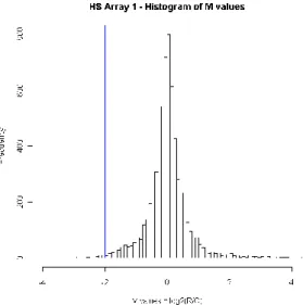
Figure 3.8 – Histogram of M-values of the first array of the HS experiment ... 30

Figure 3.9 – Fold-change: Scatter plot of the first array in the HS experiment ... 31

Figure 3.10 – Fold-change: Scatter plot of the Heat Shock experiment (six arrays) ... 32

Figure 3.11 – Fold-change: Scatter plot of the Heat Shock experiment (six arrays), log fold-change higher than 4.25 ... 32

Figure 3.12 – Not averaging spot replicates brings up different "regulated genes" ... 33

Figure 3.13 – The funnel shape ... 34

(18)

Figure 3.15 – Standard Normal Distribution: two-tailed z-test at a significance of 0.05 ... 36

Figure 3.16 – Volcano plot: t-test, p-values vs ratio log fold changes ... 40

Figure 3.17 – Volcano plot: t-test using difference log fold-changes (M-values) ... 42

Figure 3.18 – The F-distribution ... 50

Figure 3.19 – Volcano plot: ANOVA ... 52

Figure 3.20 – Volcano plot: limma ... 57

Figure 3.21 SAM Plot for the Heat Shock experiment, with delta 25.0 ... 58

Figure 4.1 – Original Mind data analysis workflow ... 68

Figure 4.2 – New Mind data analysis workflow ... 69

Figure 4.3 – The Mind application architecture ... 72

Figure 4.4 – AJAX for the design matrix creation ... 74

Figure 4.5 – AJAX for background processing ... 74

Figure 4.6 – Existing tables used for the development of the data analysis module ... 77

Figure 4.7 – New tables and associations to existing tables ... 79

Figure 4.8 – Data Set: Current Data Set ... 82

Figure 4.9 – Quality Control: Parameters ... 84

Figure 4.10 – Gene Regulation: Load normalized data, averaging spot replicates ... 85

Figure 4.11 – Gene Regulation: Filtering ... 85

Figure 4.12 – Gene Regulation: Menu ... 85

Figure 4.13 – Gene Regulation: divide by channels ... 86

Figure 4.14 – Gene Regulation: divide by arrays ... 86

(19)

List of Tables

Table 3.1 – Fold-change: HS experiment top 6 genes ... 33

Table 3.2 – Ratio and Difference Log Fold change ... 34

Table 3.3 – T-test: division of the twelve intensities of YFL014W into the control and the experiment groups ... 38

Table 3.4 – Top genes: t-test using ratio log fold changes ... 40

Table 3.5 – T-test: division of the six M-values of YFL014W into the control and the experiment groups ... 41

Table 3.6 – Top genes: t-test using difference log fold changes (M values) ... 42

Table 3.7 – The multiple comparison problem: probability of getting at least one FP raises with the number of independent tests. ... 43

Table 3.8 – Paired T-Test ... 45

Table 3.9 – Gene YFL014W: division of the M values into groups A, B and C ... 47

Table 3.10 – ANOVA: startup data for gene YFL014W ... 47

Table 3.11– ANOVA table for gene YFL014W ... 49

Table 3.12 – Design Matrix: Heat Shock Experiment ... 53

Table 3.13 – Design Matrix: ApoAI Experiment ... 55

Table 3.14 – ApoAI Experiment: TopTable of Fit, 6 genes ... 56

Table 3.15 – ApoAI Experiment: TopTable of Fit, 6 genes, coefficient 2 ... 56

Table 3.16 – Limma: HS experiment top table (10 genes)... 56

Table 3.17 – Ranking of genes by fold change method and by Limma ... 57

Table 3.18 – HS Experiment: SAM regulated genes (delta 25.0) ... 59

(20)

(21)

Acronyms and Abbreviations

ADF Array Description File

AJAX Asynchronous Javascript and XML

C Control

DB Database

DNA Deoxyribonucleic Acid

GAL Gene Annotation List

GUI Graphical User Interface

HGP Human Genome Project

HS Heat Shock

IDE Integrated Development Environment LIMS Laboratory Information Management System

MIAME Minimum Information About A Microarray Experiment Mind Microarray Information Database

PCR Polymerase Chain Reaction

QC Quality Control

RNA Ribonucleic Acid

mRNA messenger RNA rRNA ribosomal RNA tRNA transfer RNA

SNP Single Nucleotide Polymorphism

SQL Structured Query Language

URL Uniform Resource Locator

(22)

(23)

Chapter 1 Introduction

1.1 The emerging of Genetics and Bioinformatics

The completion of the Human Genome Project (HGP) in 2003 represented an amazing accomplishment in the genetics and the bioinformatics fields [1]. The sequence of bases of the human DNA (deoxyribonucleic acid) was determined, and the more than 20,000 human genes on the sequence were mapped. The project was finished quicker than expected due to the rapid advancements on the available technology.

The genetics subject has its foundation on the work of Gregor Mendel in the 19th century. He studied the inheritance of several physical traits through generations of pea plants, designating as factors the elements that transmit the phenotype information from living organisms to their offspring [2]. Later, various studies and experiments carried out by different scientists during the first half of the 20th century allowed identifying DNA as the cell component that contains the hereditary information [3]. What Mendel described as factors are the genes present in the DNA. In 1953, Watson and Crick presented the first three dimensional model of the DNA molecule, which has not changed much since then [4]. With these discoveries, the genetics area expanded quickly and is today a major field of research.

The quick progression of the genetic field cannot be dissociated from the evolution of information technology. Not only the HGP depended on it, but most research and work is done with the aid of computerized means. Molecular biology in general (the study of biology at a molecular level) which overlaps genetics, biology and chemistry, is highly dependent on computers. The relationship between these two is so cohesive that it earned its own designation – bioinformatics, a term coined by Paulien Hogeweg in 1978 to express the application of information technology to molecular biology [5].

Although it represents a big milestone, the sequencing and mapping of the human genome leaves much work to be done, in order to use this information for developments in medicine and

(24)

other fields of application. Namely, the function of the human genes, and how they work together, is an important topic of research.

Genomes of other organisms have been sequenced and mapped as well, such as the

saccharomyces cerevisiae, the yeast used in bread, beer and wine production. Although a

unicellular living being, its genome has 7,000 genes, and many of these genes overlap in sequence and in function with the human genome, providing a reason for the yeast genome to be studied extensively.

1.2 DNA microarrays for gene expression analysis

DNA microarrays are an important technology used in the research of gene function and interactions. They started to be used for gene expression analysis around 1995 [6]. All of our cells have the same DNA, but the genes that are active at a time depend on the cell type, activity and other conditions such as nutrition. Besides, genes are not just simply expressed or not, but rather more or less expressed. Given a sample of cells, DNA microarrays allow to probe the state of a group of genes within that sample.

A typical example is testing a drug for a specific disease. If a group of genes related to that disease is known, one can use this technology to evaluate the effect of the drug in those genes, comparing a group of patients that are being treated with it versus patients that are not. Genes found differently expressed between the two samples may be due to the effect of the medication. If the medication is found to inhibit a gene whose over expression caused the disease while not interfering on the other genes, the experiment will demonstrate evidence of its effectiveness.

DNA microarrays for gene expression analysis use the central dogma of molecular biology, which states that expression of genes is related to the mRNA (messenger ribonucleic acid) molecules produced in the cell during protein synthesis. mRNA molecules are another cell component like DNA. In general each mRNA molecule is one "copy" of an active gene of the DNA. The more expressed a gene is in a cell at a time, the more mRNA molecules will be available in a cell, to allow the protein synthesis necessary to carry out the function coded by the gene. Thus, given a sample of cells, such as blood or tissue, to analyse gene expression using DNA microarrays, what is measured is the mRNA extracted from the cells.

This technology can be used to study gene function and discover genes that work together, known as exploratory analysis, or to probe for genes that are expressed differently between two

(25)

(or more) samples, such as the example drug testing experiment described. The focus of this project and this document will be the latter, known as analysis of gene differential expression or gene regulation.

When using DNA microarrays to assess gene differential expression, knowledge from the areas of genetics and biology, computer science and statistics are combined together towards the goal of obtaining a list of genes that are regulated. The DNA microarray itself usually consists of a glass slide onto which the genes or probes are printed. Each slide has up to approximately 20,000 probes and an experiment can have different slides and a few replicates of each one; as a result, this represents an enormous amount of data to be processed, managed and stored.

1.3 The Mind Project at the University of Aveiro

The Mind project (Microarray Information Database) was created at the University of Aveiro, to address microarray data management and processing. It is a repository of microarray experimental data that also allows the processing of the data. This web application, hosted at http://bioinformatics.ua.pt/mind/, is a microarray dedicated LIMS (Laboratory Information Management System) and a microarray data analysis application [7].

The LIMS module is responsible for storing and organizing the data according to the MIAME standard (Minimum Information About a Microarray Experiment). As there are many manufacturers of microarray software and laboratorial equipment, this standard ensures that when a microarray experiment is performed, a common set of information is stored, such as the raw data format and the laboratorial practices used, as much information as it is needed to replicate the experiment and to understand how the available data was obtained [8].

The data analysis module processes the raw data that was submitted using the LIMS. It already contains quality control functionalities, including normalization. Quality control is the first step of microarray data analysis (common to both gene regulation assessment analysis and exploratory analysis), and it aims to remove systematic biases and to confirm the quality of the arrays. If after being subject to quality control the data appears to be of bad quality, the microarray experiment may have to be redone. Using the quality control reports generated, which consist mainly of graphical plots, the user can verify if each array was successful [9].

(26)

1.4 Objectives

The goal of this project is to continue the analysis of the normalized data. Currently, Mind is used to store the raw data files, to perform quality control and to store the normalized files. The subsequent analysis, required to assess the regulated genes, must be done with other software. This project intends to incorporate gene regulation assessment functionalities in Mind. In order to accomplish this, a study of microarray data analysis and an inquiry of available microarray data analysis tools must be done. This dissertation will thereby, besides describing the integration of the new functionalities in Mind, reveal the study that was done on microarray data analysis methods and software.

GeneBrowser is also a project developed at the bioinformatics group of University of Aveiro, like Mind. The web application, hosted at http://bioinformatics.ua.pt/genebrowser2/, given a list of genes, is able to assess their biological function, for example, by identifying them in pathways (a metabolic pathway, in biology, is a series of reactions that occur in succession towards a common goal, for example, the glycolysis pathway in yeast, which transforms sugar into piruvate) [10].

The new Mind data analysis module, object of this dissertation, will allow, in addition to performing quality control (already implemented), post-normalization analysis of the data in order to obtain a list of differentially expressed genes that can be directly and transparently exported to GeneBrowser. As Mind and GeneBrowser are both web applications, Mind can offer a link to send the list of regulated genes as input for GeneBrowser. Mind was initially designed with the inclusion of this data analysis module in it, which will provide a connection between the two web applications.

1.5 Structure

The next chapter introduces some biology theory necessary for the understanding of the DNA microarray technology as an estimate of gene expression. The microarray technology is also presented.

The third chapter, DNA Microarray Data Analysis, the longest chapter in this document, describes the methods used to derive significant meaning from the raw microarray data. As there are many methods available, the ones that were chosen for Mind will be described. However, as these correspond to the most commonly used methods, the chapter is a

(27)

considerably general microarray data analysis description. Programming libraries that offer the selected methods, and that will be used in Mind, are also presented.

The fourth chapter provides an overview of some existing microarray data analysis software solutions. Together with Mind’s users’ opinions, these provide an important insight on what is expected in a microarray data analysis application.

The fifth chapter focuses on the development of the Mind microarray data analysis module, and includes technologies used, the modifications done in the Mind application and database and presents the final result with some screen captures.

The last chapter summarizes the work done, presents the most important conclusions of this project and leaves some suggestions of future developments.

(28)

(29)

Chapter 2 DNA Microarrays: Principles and

Technology

The DNA microarray technology relies on the complementarity of bases observed in DNA and RNA molecules, the nucleic acids. This principle allows two strands of DNA or RNA to bind, if they are complementary. An mRNA sequence is complementary to the gene it was transcript from and it will bind to a sequence that is identical to the original gene.

By using DNA microarrays for gene expression profiling, the mRNA extracted from sample cells is analyzed and used to infer about the sample’s gene expression.

In order to explain these two concepts, binding of complementary sequences and mRNA as an indicator of gene expression, this chapter will begin by describing the DNA and RNA molecules, the nucleic bases, base complementariety and the role of mRNA in protein production. Finally, it will be shown how these biological principles apply to DNA microarrays with the description of a microarray experiment.

2.1 DNA and protein synthesis

From the instant we are conceived, our brief existence being unicellular, the DNA molecule residing in the nucleus of that single cell contains all the information needed to build the proteins that will form ourselves. When cell division and replication occur, obviously necessary to our growth, but always needed for tissue regeneration, the DNA molecule too is duplicated, in a much complex process, the DNA replication. Our genetic information, contained in our DNA, defines our physical and psychological traits. DNA is referred commonly as our biological identification because it is unique in each individual. All humans have the same genes, but a small percentage of the genome differs in sequence from person to person; these are the genes that describe each individual’s specific characteristics. All living beings have their DNA coding their particular characteristics. The most important biological process that describes how the information of our DNA determines what we are is the protein synthesis.

(30)

2.1.1 The DNA molecule

The DNA molecule has the form of a double helix, and each of the two strands is a sequence of nucleotides, as represented in Figure 2.1. A nucleotide is made up of a phosphate group, a pentose sugar and a nitrogenous base. The latter, in the DNA molecule, can be an adenine, a thymine, a cytosine or a guanine, and it is what distinguishes the nucleotides. In fact, the nucleotides are commonly called just by the initial of their base, A, T, C or G.

Figure 2.1 – The DNA molecule [11]

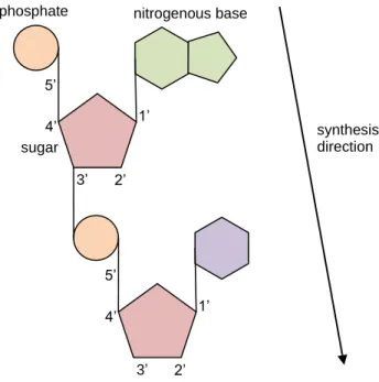
On each DNA strand, the pentose sugars and the phosphate groups connect to form the phosphate sugar backbone – the phosphate of the fifth carbon of the sugar of one nucleotide connects to the third carbon of the sugar of the following nucleotide. DNA is actually synthesized in this order, phosphate of the carbon 5 bound to the carbon 3 of the next nucleotide; it is synthesized in a 5’ to 3’ direction (five prime to three prime), as illustrated in Figure 2.2.

The bases of each strand form non-covalent hydrogen bonds with the bases on the other strand, due to base complementarity. A and T bases are complementary with one another, as are C and G. Each two complementary bases is a base pair. Two strands being complementary to one another means that the base sequence on one strand matches the base sequence on the other, allowing for the hydrogen bonding between each base pair.

(31)

ATCG is also known as the DNA alphabet, because using these four letters we can describe a DNA molecule. Figure 2.3 shows a simple representation of a DNA fragment. The parallel lines do not need to be present, they represent the backboned formed by the pentose sugars and the phosphate groups on each strand. The numbers 5 and 3 at the end of each strand indicate the direction of the strand. The top strand runs from 5’ to 3’ (five prime to three prime), the bottom strand runs from 3’ prime to 5’ prime, which is why the two strands are called anti-parallel.

Given any DNA strand, regardless of the length, one strand is expected to bind to it, the complementary strand. However, a single nucleotide polymorphism (SNP) may occur, meaning that even if the strands are not totally complementary they can still bind, so the binding of two strands does not guarantee they are totally complementary.

2.1.2 DNA and RNA – the nucleic acids

In an eukaryotic cell, the DNA resides in the nucleus. In a prokaryotic cell there is not a nucleus and the DNA is located in a region called a nucleoid, not delimited by a membrane. In fact, the words prokaryotic and eukaryotic come from the Greek language: prokaryotic means "before

3’ 1’ 2’ 4’ 5’ 1’ 2’ 3’ 4’ 5’ synthesis direction phosphate sugar nitrogenous base

Figure 2.3 – Complementarity of bases between two, anti-parallel, DNA strands

5'

ATTACGGC 3'

3' TAATGCCG 5'

(32)

nucleus" or without a nucleus and eukaryotic means "true nucleus". Prokaryotic cells are smaller and less complex than eukaryotic cells. Most organisms are eukaryotes. Humans, animals, plants, mushrooms and yeast are eukaryotes. Bacteria are prokaryote organisms. Figure 2.4 shows where DNA is located in a prokaryotic cell and in an eukaryotic cell.

Figure 2.4 – Prokaryotic and Eukaryotic cells [12]

The other nucleic acid present in the cell is the RNA. The designation (nucleic) is due to their role, and not their presence, in the cell nucleus. Although DNA always resides inside the nucleus, RNA can be in the nucleus or in the cytoplasm (in eukaryotic cells). While DNA is double-stranded, RNA is one stranded, at least in the majority of its biological roles (not including the induced mRNA/DNA hybridization on the microarrays). In RNA the nucleotides can have bases A, C and G, like DNA, but instead of thymine, RNA has uracil (U). Also, while DNA contains the sugar deoxyribose, RNA contains ribose.

An RNA molecule can bind with a DNA strand, forming a DNA/RNA hybrid, as long as the two strands are complementary (and anti-parallel). This principle is used on DNA microarray technology – the mRNA extracted from the sample is applied over the slide, and left to bind to the DNA probes.

A prefix is used to indicate the RNA function in the cell. mRNA for messenger RNA, tRNA for transport RNA and rRNA for ribosomal RNA. These three are involved in protein synthesis; there are more types of RNA for DNA replication and other cell functions.

(33)

2.1.3 Protein synthesis

Messenger RNA, mRNA, is a copy of the DNA, carried from inside the cell nucleus to the ribosomes in the cell cytoplasm, where protein synthesis will occur. This process consists of three main phases: transcription, processing and translation [13].

Protein synthesis starts with transcription, a process that forms a RNA sequence, using a DNA strand as a template. This is done in presence of an enzyme complex, the RNA polymerase. The DNA helix opens up in the region to be transcript, and the RNA polymerase slides along the DNA template strand, building, one nucleotide at a time, a complementary RNA strand. Figure 2.5 shows an example portion of the DNA molecule that is transcript and the resulting mRNA molecule. The RNA polymerase glides along the bottom strand in the direction 3’ to 5’, so the mRNA synthesis can occur from 5’ to 3’ (nucleic acids are always synthesized 5’ to 3’).

The formed mRNA is processed, to remove information that is not further on relevant for protein synthesis and then it is let out into the cell cytoplasm, crossing the cell’s porous nucleus (in eukaryotic cells).

Once in the cytoplasm, translation occurs, involving ribosomes and tRNA. The ribosomes are made of rRNA (ribosomal RNA) and protein. The tRNA (transfer RNA) are molecules that contain a sequence of three nucleotides (three of A, U, C, G) called a codon and an amino acid that corresponds to that sequence. Amino acids are the building blocks of proteins. There are around 20 amino acids, and 64 different sequences of 3 nucleotides, so different sequences can code the same amino acid. In the translation process, the ribosome scans the mRNA, matching for each three mRNA nucleotides, a tRNA that is complementary. As the tRNAs are attached to the mRNA, the protein is being formed, the sequence of the amino acids carried by the tRNAs. Once a tRNA’s amino acid is connected to the forming protein, the rest of the tRNA is discarded, leaving the three mRNA nucleotides free, which is why the same mRNA molecule can be used by different ribosomes at the same time. Several ribosomes can be at different locations of the same mRNA molecule, each one having its protein at a different stage of development, so one mRNA can allow for multiple copies of the same protein.

DNA: 5' ATGCCGTTAGACCGTTA 3'  top strand, coding strand, sense strand

3' TACGGCAATCTGGCAAT 5'  bottom strand, template strand, antisense strand mRNA: 5' AUGCCGUUAGACCGUUA 3'

(34)

After translation, the proteins can undergo many more and complex transformations until they are finally complete. To name some possible final results for these proteins, they may become enzymes and work inside the cell, they may become part of the cell’s structure or they may be exported outside of the cell. Not only the protein synthesis process described here is very simplified, many more alterations may be done after the translation.

2.1.4 mRNA as an indicator of gene expression

DNA encodes our physical and psychological traits in the manner that it contains the information for the protein synthesis to occur. The DNA is the same in practically all cells of an individual, but we have different cell types, that produce different proteins, according to the genes that are expressed. Gene expression and consequent protein production in a cell also varies according to its condition (nutrition, medication or temperature).

The mRNA present in a cell gives us an indication of what genes are expressed. The DNA microarray technology can be used to analyze the mRNA samples and conclude about gene expression. However, it is not an exact measure of gene expression: the mRNA present in the cell does not indicate exactly what genes are expressed. For cDNA microarrays (definition further in 2.2) there is the possibility that the experiment may not show the presence of some mRNA, or that it shows the presence of mRNA without it being in the sample. The probability of failing to detect present mRNA is around 5% (false negatives) and the probability of detecting mRNA that truly is not present is around 10% (false positives) [14].

It is questioned about which method provides the best picture of functional expression: mRNA expression analysis, also know as transcriptome analysis, or protein expression analysis, referred to as the proteom analysis. The transcriptome analysis scores for high degree of sensitivity, speed and completeness, but there may be discrepancies between the genes and the ultimate phenotype. For example, the butterfly and the caterpillar have identical genomes but very different proteomes. In the end, both techniques are important and complementary. The choice of one or the other depends on the biological question being asked and the resources available, but both methods are important [15].

2.2 A DNA Microarray Experiment

A microarray experiment starts with the identification of a problem that can be solved using this technology and by defining a design for a microarray experiment that will provide an answer. The experiment design describes what probes to use on the slides, what mRNA samples to

(35)

hybridize to the slide probes, how the samples will be prepared, and what information is to be collected from the experimental procedure. After proper planning, the experiment can be carried out: the microarrays are prepared, hybridization of the targets and the probes occur and the microarrays are scanned. The resulting pictures of the microarrays are converted to numerical data that is handled with data analysis. Figure 2.6 enumerates the steps of a microarray experiment.

2.2.1 The microarray slides and probes

The microarray slide can be of different materials, and the probes can be placed on the slide using different methods. The most common are spotted arrays, which use high quality glass slides. The probes are produced and then they are spotted onto the slide, using a spotting robot. This machine dips a grid of fine pins into the wells containing the probes and then lays the tiny drops onto the microarrays slide. Spotted microarrays can be cDNA (most commonly) or oligonucleotides, depending on how the probes were produced [16, 17]. cDNA sequences are cloned from a known gene using a DNA or RNA strand as a template and can be thousands of nucleotides long. These sequences are multiplied, usually using a technique called polymerase chain reaction (PCR), as each spot on the microarray requires thousands of copies of the same cDNA sequence. Oligonucleotide sequences are shorter, up to 20 nucleotides, and are not produced in a laboratory like cDNA sequences. At the University of Aveiro Biology lab, oligo (short for oligonucleotide) sequences are purchased from a manufacturer and then, in the lab, they are spotted onto the microarray slides. Manufacturers also provide complete arrays, with the oligo sequences already printed onto the slides.

There is not a clear definition of cDNA and oligo arrays in the literature. Oligo arrays are sometimes associated to one-color arrays, and cDNA to two-color arrays, but there are two-color arrays with oligo sequence probes. Oligo arrays are usually associated to the commercial arrays, but they can also be printed in the lab, although the oligo sequences must be purchased first. Commercial arrays (purchased with the probes printed) are normally produced using in situ synthesis, thus the term oligonucleotide is associated with this manufacture method

Experiment Design Microarray Acquisition or Preparation Target Preparation. Hybridization and Scanning Data Analysis

(36)

too. The in situ synthesis is a method, usually based on photolithography (involving light and light-sensitive masks), that synthesizes the probe sequences directly onto the array surface.

At the Biology department of the University of Aveiro, spotted cDNA microarrays are produced in the lab, oligo sequences are purchased to be spotted in the lab and commercial complete oligo arrays are acquired too. In all cases, the arrays are used as two-color, allowing hybridization of two mRNA samples on each slide, labeled with two different color fluorescent dyes.

Figure 2.7 – Microarray glass slide, spotter and commercial array [18-20]

2.2.2 Target preparation, hybridization and scanning

After planning the experiment and arranging the microarray slides, the biologist prepares the mRNA samples or targets. The mRNA is extracted from the cells to be studied. For each array, two mRNA samples are used and each one is labeled with a different color fluorescent dye. Commonly cyanines cy3 (green) and cy5 (red) are used. The two labeled mRNA samples are applied over the slide and let to hybridize in a hybridization oven, which provides optimum conditions for the process. The mRNA will bind to the spots whose probe sequences are complementary.

Once hybridization is complete, the slides are read by a microarray scanner. The scanner’s light excites the red and green fluorescent dyes. Spots to which mostly the red labeled mRNA sample has bound will glow red, spots that contain mostly the green labeled mRNA samples will reveal a green color, and spots that have about the same amount of both will be yellow. Color intensities also vary, from bright colored (red, green or yellow) to black, indicating how much mRNA was actually fixed. The scanner will output an image showing the hybridization that occurred in the slide.

2.2.3 Raw data files: the starting point to microarray data analysis

The images obtained from the scanner are processed using microarray image analysis software, provided from the scanner manufacturer or available separately. The software produces one data file for each image and for each scanned array (Figure 2.8). It is usually a tab delimited text file,

(37)

with as many rows as the spots of the microarray and several columns for the spot attributes. The most relevant fields are the red and green mean intensities and the red and green background intensities. These values do not have units, but they range from zero to tens or hundreds of thousands. The foreground intensities indicate how much red and green is measured in each spot as a consequence of the competitive hybridization. The background intensities show how much red and green was measured just outside the circular area of each spot, consequence of noise, non-specific hybridization or other factors.

Figure 2.8 – From microarray image to raw data file

A GAL file (Gene Annotation List) must also be created, describing what gene is probed on each spot. The MAGE-TAB equivalent, ADF (Array Description File), contains the same information, where MAGE-TAB is a MIAME-compliant format for organizing microarray experimental data [21]. Both GAL and ADF describe the array layout. Figure 2.9 shows an example array layout, consisting of 4 × 12 squares of 20 × 20 spots each, for a total of 19200 spots. The GAL or ADF file for this array would indicate the name of the gene relative to each spot, just like the data files, it also contains as many rows as the number of spots in the array.

Figure 2.9 – Example array layout

Once the array layout file and the data files are obtained, the microarray data analysis begins. The first part of data analysis is quality control. Quality control includes background correction and normalization procedures, and in addition to correcting the data for systematic biases and noise, it allows acknowledgement that the arrays were successful. If even at the end of this step the data is of bad quality, then the microarray hybridization and/or scanning must be done again until the normalized data for all arrays is acceptable. The second part is gene assessment analysis, which aims to find genes that are likely to be differentially expressed between the samples under study. Alternatively, instead of gene regulation analysis, exploratory analysis could be done, to discover unknown genes or to learn about groups of genes that work together, involving procedures like clustering of the gene expression values; this dissertation will

indexs Gmean Rmean bgGmean bgRmean … 1 65264 65226 508 393

2 681 600 514 391 3 521 406 461 342 4 540 417 468 348

(38)

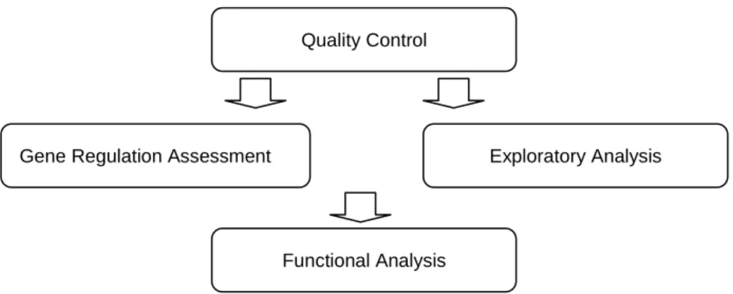
approach the former. After gene regulation assessment (or exploraroty analysis) functional analysis can take place (Figure 2.10). Exploratory analysis is not contemplated at the moment, but may be added to Mind in future developments. This project adds gene regulation analysis to Mind, constituting itself as a bridge between the existing Mind quality control functionalities and GeneBrowser’s functional analysis.

2.3 Summary

This chapter exposed essential biology theory for the comprehension of the microarray technology. The hybridization on the microarray slides occurs due to complementarity between the probe and the target strands. The mRNA is measured to infer about gene expression in the sample. A microarray experiment was presented, including the preparation of the slides, the probes and the targets, the hybridization and the scanning of the microarrays, and the conversion of the image files to raw data files. With the raw data files and a GAL or ADF file, descriptive of the array layout, the microarray data analysis may begin.

Quality Control

Gene Regulation Assessment Exploratory Analysis

Functional Analysis

(39)

Chapter 3 Microarray Data Analysis

The previous chapter presented an overview of the basics of the microarray technology and the initial steps of a microarray experiment, up to the acquisition of the raw data files. The present chapter will go through the fundamental theory of microarray data analysis, for both quality control and gene regulation assessment phases, focusing on the functionalities that were chosen for Mind, as there is not only one exact way of performing microarray data analysis. However, this chapter still exposes a fairly general microarray data analysis approach, and not Mind-specific, because the described methods are some of the most commonly used ones in microarray data analysis and recurrent in related literature. Despite many methods being available for both quality control and gene regulation assessment, only a small percentage is actually used in the majority of experiments.

In Mind, most data analysis functions are offered using R libraries. It is better to use functions that are already available instead of writing new code, especially as the analysis methods are complex algorithms. R is a statistical framework that allows data processing, plot generations, and more [22]. It has its own windows environment or it can be run from the operating system’s command line. In both cases data processing and plot generation is done with the R scripting language. This makes R ideal to execute scripts from an application, which is what is done in Mind: the website site provides a GUI to the user, and using his input, processes the microarray data with R. This software is open source and it can be downloaded from the Comprehensive R Archive Network website (CRAN). R base functions are the ones that come with the downloaded software and include arithmetic operations, plots, statistical methods and more. Additional libraries or packages can be downloaded and installed into R, such as libraries specific for the analysis of microarray data. Many bioinformatics related R libraries are released under the Bioconductor project. More information about R and Bioconductor will be presented in the application development chapter (Chapter 5). This brief introduction was required as the current chapter, by introducing the microarray data analysis methods, will present the specific R libraries selected for the Mind R scripts.

(40)

Data of a DNA microarray experiment performed at the University of Aveiro Biology department will be used as an example. This experiment aimed to study the result of submitting

saccharomyces cerevisiae cells to a heat shock. The yeast cells initially were at a temperature of

30 ºC, and they were left to incubate at 37 ºC for twenty minutes. mRNA samples of the cells were taken, before and after the incubation at 37 ºC, leading to two conditions: the "before" or "control" sample and the "after" or "experiment" sample. The heat shock effect on yeast cells is a phenomenon that has been studied thoroughly, either with DNA microarrays or other tools, and many references are available on this matter [23]. This experiment was performed at the lab mainly to check the microarray technology and experimental protocol being used by ensuring the results are as expected. In this chapter, it will be shown how after performing microarray data analysis on the heat shock experiment raw data, a list of regulated genes is obtained.

For the heat shock experiment three biological replicates were used, meaning that the heat shock was applied to three different cultures of yeast, developed under the same conditions, but in three separate containers, yielding the mRNA samples C 1, 2 and 3 (Control), and HS 1, 2 and 3 (Heat Shock). For each distinct culture, two microarrays were created, which are technical replicates. Each pair of technical replicates are also dyes-swaps, meaning that on one array the green channel is assigned to the control and the red channel to the heat shock, and on the other array these are swapped. Dye swap technical replicates are used to make up for different dye efficiencies. Figure 3.1 shows the diagram of the microarray experimental design. Whether the arrows are colored or not, it is a convention that their direction goes from the green labeled sample to the red labeled sample.

Figure 3.1 – Heat Shock microarray experiment design

The comparison will be done between the control and the heat shock groups, to assess differential expression between the two. A gene that shows a very high intensity on the heat shock group and a low intensity on the control group will be classified as upregulated. A gene that is much less expressed on the experiment group will be downregulated.

Using the heat shock data, this chapter will clarify some necessary concepts like spot and gene expression values and graphical plots used and will then detail the quality control and the gene regulation assessment phases of data analysis. Greater emphasis will be placed on the latter, as quality control was already implemented at the beginning of this project. Although the quality control module is to be revised, its functions, mainly offered through Limma, are suitable for Mind’s users and will not be changed.

(41)

3.1 Expression Values, Scatter Plots and MA Plots

For one microarray, one may plot the green intensities against the red intensities. The originated plot, the scatter plot for that array, shows most spots are scattered along the x = y line, meaning most spots have similar intensities in both samples. Given two conditions, like the control and the heat shock conditions in the example experiment, there are not expected to be many regulated genes. The same applies if comparing a healthy and disease tissue or a medicated and placebo tissue. In fact, gene regulation assessment with DNA microarrays uses this principle as an underlying assumption: most genes will not be differentially expressed among the conditions under study and the goal is to investigate the few genes that are. Scatter plots can be taken for one microarray, for a subset of spots or genes or for multiple arrays (by averaging intensity values across them), as long as two groups of expression values can be plotted one against another.

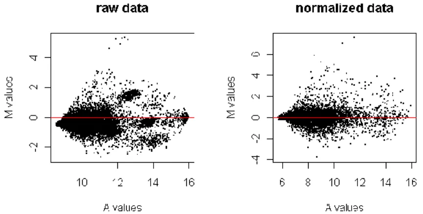
Scatter plots are taken using the logged intensities. Figure 3.2 shows that this transformation permits a more even distribution of the values along the graphic area and a better reading of the graph too. The last plot, with normalized data, shows the spots scatter better along the x = y line. Before quality control, red and green intensities may show a systematic discrepancy from the x = y line, due to some technical issue that may have affected in the same manner all intensity values.

Figure 3.2 – Scatter plots of the first array of the Heat Shock experiment

In two-color microarrays, a spot’s or a gene’s expression value is the M-value, the base two logged ratio of the red and green intensities. A spot represents a single location on the microarray grid while the gene’s expression value is the average of the expression values of all spot replicates that refer to that gene. It should be avoided to consider the individual red or green intensities on their own because they result of competitive hybridization. The intensity a spot shows on the red channel depends on the mRNA present on the red labeled sample, but

(42)

also on the mRNA present on the green labeled sample too. For two-color array data, the M-value is the appropriate gene expression value, with the R/G ratio, and not the individual red and green intensities:

M-value= 𝑙𝑜𝑔2

𝑅

𝐺 = 𝑙𝑜𝑔2 𝑅 − 𝑙𝑜𝑔2 𝐺

The ratio in M-values, along with reflecting best the result of the competitive hybridization in two-color arrays, allows comparison of spot expression on one mRNA sample with the other. A gene with an intensity of 10000 on the red sample and an intensity of 1000 of the green sample has the same relative expression as a gene with a red intensity of 1000 and a green intensity of 100; they both have a 10-fold-change. The ratio is logged so that up and down regulation is accounted similarly. A gene that is 100 times more expressed on the red mRNA sample has a ratio of 100, but a gene that is 100 times more expressed on the green mRNA sample has a ratio of 0.01. By taking the logarithms, the first gene has an M-value of 2, and the second gene has an M-value of -2. If expression values were given by ratios only, there would be a [1,∞[ range for the genes up regulated in the red sample and a [0,1] range for the downregulated genes. M-values allow ranges of equal dimensions for both cases: ]∞,0] for downregulation and [0,∞[ for the upregulation. Logarithms also allow more perceptible plots by distributing the spots more evenly. Figure 3.2 showed how the scatter plot became more perceptible by logging the individual intensities and the same effect is obtained by logging the intensity ratios. Logarithms are taken in base 2 for a matter of convenience, in subsequent data analysis. For example, later in this chapter the fold-change gene regulation assessment method will be explained, a method that easily selects genes that have a fold-change higher than 4, by selecting M-values with absolute value higher than 2; the square of 2, the log fold-change, provides the fold-change value, which is 4 [24-26].

MA plots are two dimensional graphical plots that plot the M-values (expression values, intensity ratios) of a set of genes against the A-values (average intensity values). The average intensity of a spot is given by

A-value = 0.5 × 𝑙𝑜𝑔2 𝑅 + 𝑙𝑜𝑔2 𝐺 = 0.5 × 𝑙𝑜𝑔2 𝑅 × 𝐺

An MA plot can be generated for the spots of one microarray, for several arrays (by averaging the red and green intensities, or the control and experiment intensities, and then taking the M-values) or for a smaller selection of spots or genes. Figure 3.3 shows the MA plots for the first array of the heat shock experiment, before and after quality control. In both cases, the plot shows a bigger concentration of spots around the M = 0 line, although after quality control

(43)

scattering along this line is more evident. Most genes of a sample in two different conditions are not differentially expressed. The aim of gene regulation assessment is to find the small fraction of regulated genes that are.

Figure 3.3 – MA Plots of the first array of the Heat Shock experiment

3.2 Quality Control

Once the raw data files are obtained, quality control must be performed on the data, involving preprocessing and normalization functions that allow the data to be corrected for systematic biases, such as noise, and the user to check the quality of the arrays. If the data does not look as expected after quality control, which the user can see using the graphical plots generated, than the microarray scanning and/or hybridizations must be done again.

According to some references, normalization can be considered part of preprocessing the data, and thereby quality control and preprocessing would be synonyms. Other references consider preprocessing the filtering and background correction functions and not normalization. It can be simply said that quality control is the collection of all the filtering, background correction and normalization functions applied to the raw data. In this phase, the arrays are separately, and within each array, the spots are handled individually, regardless of the spots being replicates referring to the same gene or not.

It is very important to perform quality control as microarray experiments are typically very noisy and various factors can affect deeply the data. Whether the next step is exploratory analysis or gene regulation assessment, it is important to have the expression values as accurate as possible, in order to infer conclusions out of it. If the influence of systematic factors is minimized, then the random (biological) variability will stand out more clearly [24].

(44)

The quality control functions presented in this section (filtering, background correction and normalization) are characteristic of two-color microarray data. These quality control functions were already implemented and available in Mind prior to the beginning of this project, and they have been meeting Mind users’ needs adequately. All of them, except for filtering, are offered through the R Bioconductor library Limma. This package, mostly known for its gene regulation assessment functions, also contains a great selection of functions to perform quality control on two-color array data.

3.2.1 Filtering

Filtering allows discarding spots that do not seem of interest. This first filtering is not "permanent"; it does not go beyond quality control. Gene regulation assessment will have its own (and a little different) filtering functions. Spots discarded by quality control filtering will still be available for gene regulation assessment. Quality control filtering is used to generate the quality control plots. At the end of quality control, the user will evaluate the quality of the arrays based on MA plots, one plot for each array. A microarray has tens of thousands of spots, so the user may choose to filter out the spots that are barely expressed and that most likely will not be relevant. Figure 3.4 shows how the MA plot of normalized data of the first array of the heat shock experiment, also shown previously in Figure 3.3, is plotted with an intensity filter that selects spots with one or both intensities higher than 1000. Quality control filtering is intended to generate clearer MA plots so the user may concentrate on analyzing the shape of the plot considering the high intensity plots. Again, all data will still be available for gene regulation assessment.

Figure 3.4 – MA Plots: the effect of filtering out low intensity spots

The issue that calls for filtering is as follows. Spots with low red and green intensities can be taken as highly expressed. A spot with a red intensity of 100 and a green intensity of 1 is a low intensity spot, as intensities usually range from zero to tens or hundreds of thousands. However, these intensities suggest the gene is one hundred times more expressed on the red sample and lead to the high M-value of 6.64. In two-color array data, the expression value of a spot is the

(45)

ratio of the red and green intensities, but for low intensity spots these ratios may be misleading. The intensity values are so low that they be due to noise and the gene may better be classified as equally and non-expressed in both samples. Low intensity spots, even if they show high M-values, are hardly relevant when the objective is selecting regulated genes. To prevent these genes from figuring in the regulated gene list the user must perform post-normalization filtering, but if he wishes to clear the quality control graphical plots from low intensity spots he must perform filtering in this phase.

Filtering by intensity selects only the spots with big enough red and/or green foreground intensities. Filtering by signal to noise (S2N) ratio selects only the spots whose red and/or green foreground intensity is much bigger than the background intensity. Both these filters are implemented in Mind’s quality control module. In practice, both filters, intensity and signal to noise ratio, will lead to similar results – spots with high foreground intensities usually have high signal to noise ratios, and can be selected with any of the filters. For example, in the first array of the Heat Shock experiment, the selection of spots with one or both of the intensities higher than 2000 overlaps considerably with the selection of spots with one or both of the S2N ratios higher than 5, as shown in Figure 3.5.

Figure 3.5 – Intensity and S2N ratio filters overlap

One of the columns of the raw data file is a bad spot flag created by the image analysis program to indicate spots that are of bad quality in a way that the intensity values cannot be reliably provided, although there should not be many such spots in an experiment. In the Mind R scripts, this column is read from the raw data files too and treated by Limma as weights that are taken into account during normalization. Limma’s handling of bad spots is transparent to the user and independent from the quality control filtering described, and its purpose is also different. The quality control signal to noise ratio and intensity filters do not affect data normalization at all, just the spots that appear on the graphical plots.

(46)

3.2.2 Background correction

The image analysis program provides data for each and every spot of a microarray (as shown previously in Figure 2.7). The attributes of a spot include red and green foreground and background intensities. The foreground intensity referrers to the spot’s total measured intensity in the red or green channel. The background intensity is the ambient signal measured, a result of non-specific binding and spatial heterogeneityacross the array.

The background intensity, detected by the microarray scanner and measured by the image processing software, can be due to several factors, such as non-specific binding of the labeled sample to the arraysurface, natural fluorescence of the glass or its coating or optical noise from the scanner [24, 27].

Background correction is the process of readjusting the foreground intensity values, taking in consideration the detected background values, providing new foreground intensities. Choosing not to use background correction means to consider the new foreground intensities equal to the original ones, thus discarding the background intensity values. In fact, some references advise not to use background correction, as it does not improve the detection of differentially expressed genes, and reduces the precision of data by increasing the variability of low intensity spots values [28].

The most intuitive and common method involves simply subtracting the background values to the foreground values, for both red and green channels, and it is referred to as the subtract or the standard background correction method. Although this method is simple and quite logical, it produces negative intensities when the background intensity detected is larger than the foreground, which in turn will lead to missing expression values (logarithms of negative values cannot be taken). The negative intensities, also referred to as "black holes", occur when the mRNA binds more to the surface than to the spot itself, causing higher non-specific binding than specific binding [29]. Some control probes may have been spotted on the microarray to ensure no mRNA binds to those spots. Although the heat shock data, in study throughout this document, has no such spots, other data may have.

Even when not missing, using background subtract may cause the log-ratios for low intensity spots to be highly variable [27]. The method most commonly subtracts the mean background intensity to the mean foreground intensity, for the red and for the green channel. This is the way it is used in Mind. But other spot attributes can be taken instead of the mean background, such as the spot’s morph value, which is a non-linear filter that provides values that are lower and less variable than the background intensity.

(47)

Improved versions of the standard method do not perform the subtraction if the result is negative. In the minimum method, in spots that would yield zero or negative values, the new intensity is set to one half of the minimum positive corrected foreground intensity for that array. In the half method, spots that would yield less than 0.5 with the subtract method are set to 0.5. These two methods are available in the Limma library and offered in Mind.

Limma also includes more complex methods, norm exp, edwards and moving minimum, which are offered in Mind. M. Ritchie et al compare and describe several methods in [27] and use them to assess differential expression, concluding that the more complex model-based correction methods perform better than the standard background subtraction.

3.2.3 Normalization

The vast majority of spots in an experiment are not differentially expressed between the two RNA samples. When comparing for example, healthy and diseased or placebo and drug treated tissues, not many genes are expected to be regulated between the pair of samples. Therefore, most spots must have equal red and green intensities and M-values around zero. In an MA plot, most genes are expected to be around M = 0. However, some kind of systematic variation that occurred during the microarray experiment may cause data to be constantly distributed differently, for example, around M = 1.

Normalization aims to identify systematic variation in the data of an array and to correct it. If all spots appear to be increased by 1 in their expression values due to some bias, then it will make sense to adjust the red and green spot intensities in order to achieve expression values that are concentrated around M = 0. This is the basic idea of normalization. It corrects the data for systematic variation, caused by different reasons such as different incorporation efficiency of dyes, different amounts of mRNA, printing or print-tip problems, so the data will express better the biological variation. Ideally a normalization method would enable the data to express only the unsystematic variation, but as it is not possible, normalization methods attempt to minimize as much as possible the effect of non-biological variation.

The Limma package implements the normalization methods that are offered in Mind: median, loess, print-tip loess and robust spline. The median method subtracts the weighted median from the M-values for each array. The other methods are more complex and are explained further in the Limma user’s guide and help manual. Print-tip loess handles data on each print tip at a time. A print-tip is each of the twelve squares shown on the example of Figure 2.8. Print-tip loess generates a curve for each print-tip using local regressions, and adjusts the intensity values according to that curve. Figure 3.6 shows this method aligns the averages per print-tip. Global

(48)

loess does a similar procedure but for the entire array. Robust spline implements an idea similar to print-tip loess, but uses regression splines in place of the loess curves.

Figure 3.6 – Print-tip loess aligns the averages per print-tip

More details about the normalization methods implemented in Limma are available in Limma help and in the article by G.K. Smyth about normalization of cDNA microarray data [30]. More information about microarray data normalization in available in many good sources, such as the introduction to Microarray Data Analysis by M. Babu [9], the book by J. Quackenbush et al [24] and the book by S. Draghici [25].

Normalization concludes quality control. Limma contains functions that generate MA plots and other useful graphics for the raw, background corrected and normalized data. Mind quality control produces one report for each array with these graphics, allowing the user to assess the quality of the arrays. It may happen that the data does not look at all like the MA plots that have been presented in this chapter, in that case something went wrong with the experiment and it must be redone. Otherwise, if after background correction and normalization the data looks adequate, the differential gene expression analysis can begin.

(49)

3.3 Differential Gene Expression Assessment

Differential gene assessment starts with averaging the spot replicates. This was not required in quality control, which intended to check the quality of each array as a whole and correct each of its individual spots for systematic bias. The present phase, using the normalized data, aims to select genes that are differentially expressed. Spots that refer to the same gene (identified by its name in the GAL/ADF file) should be averaged. This step is not strictly obligatory, although highly recommended. If spot replicate averaging is not done, than the spots will be considered independently. In this phase, the spots are no longer considered, but genes instead. Without the averaging, each spot will be regarded as a distinct gene. Simply averaging the spots disregards replicate variability, but it is currently the most commonly used method [31].

After the spot replicates averages are taken, filtering is (optionally) performed on the data. The filtering done in quality control is no longer considered, as it filtered only the spots to appear on the quality control graphical plots. Filtering on this phase will select the group of genes onto which the statistical method is applied. Finally, on the filtered genes, or on all genes if filtering was not done, a statistical method is applied to output a list of regulated genes. This section will describe filtering and will present several statistical methods. The chosen R libraries to offer the statistical methods in Mind will also be presented. The statistical methods will be exemplified using the non-filtered data, with spot replicates averaged (background corrected with the subtract method and normalized with the print-tip loess).

3.3.1 Filtering

The reason for filtering is to discard low intensity genes that can otherwise figure in the regulated gene list if they have high M-values. Quality control filters only selected spots for inclusion in the graphical plots that helped the user assess the quality of each individual microarray. A spot would be selected or not to figure in the MA plots of its array. Those were per array plots and the filters selected or excluded each individual spot.

Now the goal is to identify regulated genes. The spots are no longer considered individually, but the genes (spot replicate averages). The arrays are no longer considered separately as the genes will be declared as regulated or not based on their expression values throughout all the arrays. Filtering is now done based on the values the genes show in all the arrays. A gene cannot be selected on one array and excluded on another, either it is selected or it is not.