F
ACULDADE DEE
NGENHARIA DAU
NIVERSIDADE DOP
ORTODon’t You Forget About Me:
Enhancing Long-Term Performance in
Electrocardiogram Biometrics
Gabriel Lopes
Mestrado Integrado em Bioengenharia Supervisor: Jaime dos Santos Cardoso, PhD
Co-Supervisor: João Ribeiro Pinto, MSc
c
Don’t You Forget About Me: Enhancing Long-Term
Performance in Electrocardiogram Biometrics
Gabriel Lopes
Mestrado Integrado em Bioengenharia
Approved in public examination by the Jury:
President: Miguel Velhote Correia, PhD Opponent: Susana Brás, PhD
Referee: Jaime S. Cardoso, PhD July 17, 2019
Resumo
Hoje em dia, é esperado assegurar a integridade física, mental ou moral de um individuo. Num mundo coberto de tecnologia, a violação desta integridade é facilitada, pelo que ataques de con-trafação/ roubo de identidade são comuns. Embora os métodos atuais de segurança visem dificul-tar estes ataques, ainda não existe um sistema infálivel. Um dos método é a biometria (técnica de reconhecimento do indivíduo) que contém algumas vantagens relativamente aos metodos tradi-cionais tais como ser conveniente, redução de custos e aumento da segurança.
Esta dissertação focou na implementação de processos/ técnicas do estado-da-arte para melho-rar a performance de um sistema biométrico de eletrocardiograma em condições realistas durante um longo periodo de tempo. Distintos desafios foram encontrados para procurar a melhor solução. Foram utilizadas diversas abordagens no pré-processamento bem como na extração de caracteris-ticas para posterior avaliação.
Recorrendo a um filtro passa banda (1-40 Hz), com a aplicação da DCT na média dos com-plexos QRS (janela de 0.35 s) e com o kNN como classificador obteram-se as melhores melhorias
em média com a técnica de fixação (j× 3 + 3) Os resultados revelaram uma melhoria de 10.0%,
que apesar de ser uma melhoria significativa comparativamente com os metodos do estado-da-arte, ainda não é o suficiente para aplicações de um longo periodo de tempo.
Abstract
Nowadays, the physical, mental or moral integrity of an individual is expected to be ensured. In a technology-covered world, violation of this integrity is facilitated, so counterfeit/identity theft attacks are common. Although the current methods of security, that aim to hamper this attack, there is still no infallible system. One method is biometrics (individual recognition technique) which contains some advantages over traditional methods such as convenience, reduced costs, and increased safety technique.
This dissertation focused on the implementation of state-of-the-art processes/techniques to improve the performance of a biometric electrocardiogram system under realistic conditions over a long period of time. Different challenges were found to find the best solution. Several approaches were used in the pre-processing as well as in the extraction of characteristics for later evaluation.
Using a bandpass filter (1-40 Hz), with the application of the DCT in the mean of the QRS complexes (window of 0.35 s) and with the kNN as the classifier, the best improvements were obtained on average with the fixation technique (j× 3 + 3) The results showed an improvement of 10.0%, which despite being a significant improvement compared to the state-of-the-art methods, is still not enough for applications over a long period of time.
Acknowledgements
Contents
1 Introduction 1
2 Electrocardiographic Signal Characterization 3
2.1 Anatomy and Physiology . . . 3
2.2 Acquisition . . . 5
2.2.1 Standard Medical Acquisition . . . 5
2.2.2 Common ECG Acquisition Settings . . . 8
2.2.3 Variability . . . 9
2.2.4 Noise Contamination . . . 9
2.2.5 Right Leg Drive . . . 10
2.3 Biometrics Application: Challenges and Opportunity . . . 11
3 Machine Learning: Fundamental Concepts 13 3.1 Introduction . . . 13
3.2 Supervised vs Unsupervised vs Reinforcement Learning . . . 13
3.3 Feature Extraction . . . 14
3.3.1 Feature Extraction in ECG Biometric . . . 15
3.4 Dimensionality Reduction . . . 15
3.5 Classification Methods . . . 17
3.6 Performance Evaluation: Basic Metrics . . . 19
3.7 Conclusion . . . 21
4 Biometric Systems: Basics 23 4.1 Biometric Modalities . . . 23
4.2 Qualities of Biometric Modality . . . 24
4.3 Common Structure of a Biometric System: . . . 24
4.3.1 System Modules . . . 24
4.3.2 Operation Modes . . . 26
4.3.3 Conventional vs Continuous Biometrics . . . 26
4.3.4 Continuous Biometrics . . . 29
4.3.5 Biometric Menagerie . . . 31
4.3.6 Ideal Conditions for a thorough Performance Assessment . . . 32
4.4 System Design Considerations and Concerns . . . 32
4.5 Summary and Conclusions . . . 33
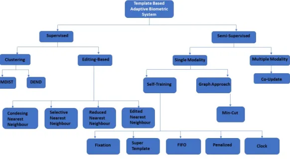
5 Adaptive ECG Biometrics Systems: Prior Art 35 5.1 Introduction . . . 35
5.2 The significance of a well-structured Signal Database . . . 35
viii CONTENTS
5.3 Long-term ECG Database . . . 35
5.4 State-Of-The-Art: Template Update . . . 36
5.5 Supervised and Semi-supervised Learning Methods . . . 38
5.5.1 Supervised Methods . . . 38 5.5.2 Semi-supervised Methods . . . 38 5.6 Clustering Methods . . . 38 5.7 Editing-based Methods . . . 39 5.8 Semi-Supervised methods . . . 40 5.8.1 Self-Update methods . . . 40 5.8.2 Graph-based Methods . . . 42 5.8.3 Co-update Methods . . . 43 5.9 Evaluation Metrics . . . 43 5.10 Model Update . . . 44 5.11 Conclusion . . . 44 6 Variability Study 45 6.1 Introduction . . . 45 6.2 Experimental settings . . . 46 6.3 Signal Pre-processing . . . 47 6.4 Feature engineering . . . 48 6.5 Classification . . . 48 6.6 Results . . . 49
7 Template Update Experiments 55 7.1 Introduction . . . 55
7.2 FIFO . . . 55
7.2.1 Threshold . . . 55
7.3 Fixation . . . 55
7.4 Adaptive Clock . . . 56
7.5 Results and Discussion . . . 56
8 Conclusion 65 8.1 Final Remarks and Future Work . . . 65
A Appendix 67
List of Figures
2.1 Heart description . . . 4
2.2 Single Heartbeat . . . 5
2.3 Einthoven Triangle . . . 6
2.4 12 Leads Configuration . . . 7
2.5 Electrode placement in the Frank VCG system . . . 8
3.1 Basic modules of reinforcement learning. . . 14
3.2 Common fiducial features extracted . . . 16
3.3 Confusion matrix . . . 19
3.4 ROC curve . . . 21
4.1 Simplest scheme of biometric . . . 26
4.2 Module representation . . . 27
4.3 DET plot . . . 30
5.1 Template update dendrogram . . . 38
6.1 Inconclusive Signals. . . 46
6.2 Signal Overlap . . . 47
6.3 Code Timeline . . . 48
6.4 Common step in ECG signal pre-processing. . . 49
6.5 Signals filtering resorting to Butterworth filter. . . 49
6.6 Signals normalization. . . 50
6.7 Signals progression according to Plataniotis method . . . 50
6.8 Tawfik method feature extraction. . . 50
6.9 feature extraction Belgacem . . . 51
6.10 Structure Auto-encoder . . . 51
6.11 Adaptive Labati Results . . . 52
6.12 Variability Results . . . 53 7.1 Ratio Plot . . . 56 7.2 FIFO Plataniotis . . . 57 7.3 FIFO Auto-encoder . . . 58 7.4 FIFO Tawfik . . . 58 7.5 FIFO Belgacem . . . 59 7.6 Backpropagation cNN . . . 59
7.7 FIFO Tawfik with kNN . . . 60
7.8 FIFO Belgacem with kNN . . . 60
7.9 FIFO cNN with kNN . . . 61
x LIST OF FIGURES
7.10 Fixation Plataniotis . . . 61
7.11 Fixation Autoencoder . . . 62
7.12 Fixation Tawfik with kNN . . . 62
7.13 Fixation Belgacem with kNN . . . 63
List of Tables
4.1 Comparison biometric trait . . . 25
5.1 Literature Databases . . . 37
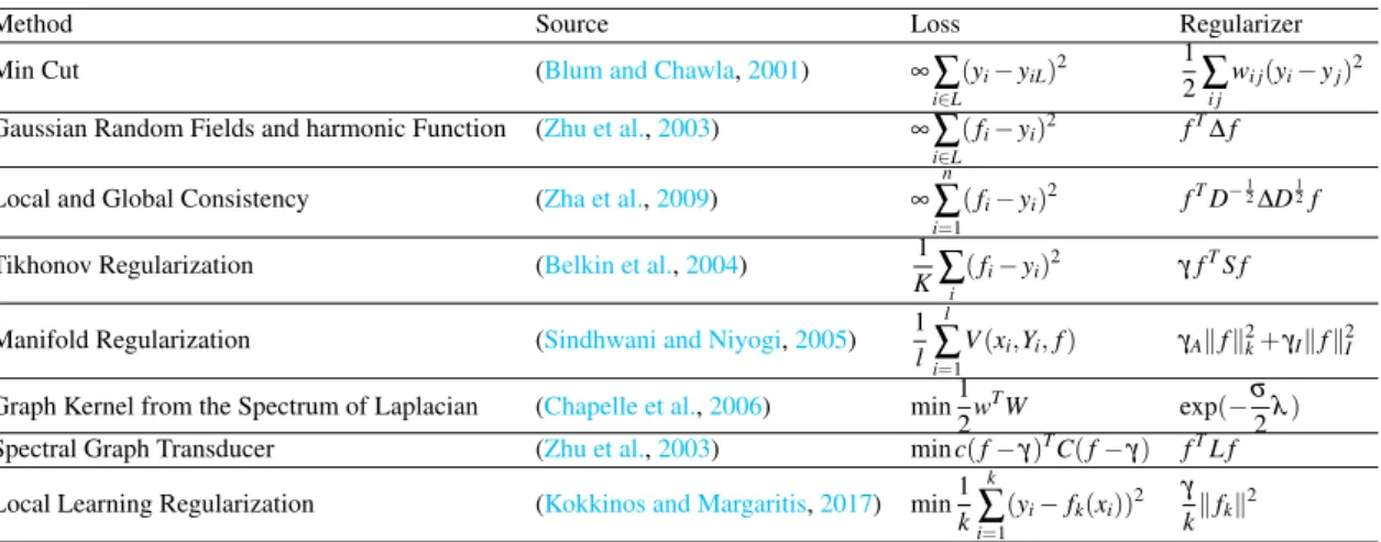
5.2 Graph-based methods . . . 42
A.1 Plataniotis results with different starting times . . . 67
A.2 Plataniotis results with rates . . . 68
A.3 Eduardo results with rates . . . 69
A.4 Belgacem results with rates . . . 70
A.5 Tawfik results with rates . . . 71
A.6 cNN results with rates . . . 72
Abbreviations
2D Bi dimensional
AC Alternating Current
ACC Accuracy
ACL Autocorrelation
ANN Artificial Neural Network
ANOVA One-way Analysis of Variance
AV Atrioventricular
aVF Augmented Vector Foot
aVR Augmented Vector Right Wrist
aVL Augmented Vector Left Wrist
AUC Area Under the Curve
BPF Bandpass Filter
BVP Blood Volume Pressure
CFS Correlation feature selection
CMC Cumulative Match Characteristic
cNN Convolutional Neural Network
CWT Continuous Wavelet Transform
DCT Discrete Cosine Transform
DET Decision Error Tradeoff
DNA Deoxyribonucleic Acid
ECG Electrocardiogram
EER Equal Error Rate
EFDT Extremely Fast Decision Tree
FAR False Acceptance Rate
FLDA Fisher Linear Discriminant Analysis
FN False Negative
FNIR False-Negative Identification Rate
FP False Positive
FPF False Positive Fraction
FPIR False Positive Identification Rate
FRR False Reject Rate
GBFS Greedy Best First Search
GUMR Genuine Update Miss Rate
HLDA Heteroscedastic Linear discriminant Analysis
HMM Hidden Markov Model
KPCA Kernel Principal Component Analysis
HRV Heart Rate Variability
IDR Accuracy
xiv ABBREVIATIONS
IUSR Impostor Update Selection Rate
kNN k-Nearest Neighbours
LBP Local Binary Patterns
LDA Linear Discriminant Analysis
LLR Log-Likelihood Ratio
LT Long-Term
MIDR Misidentification Rate
ML Machine Learning
MLP Multilayer Perceptron
MRE Mean Error
PCA Principal Component Analysis
PCG Phonocardiogram
PIN Personal Identification Number
PPG Photoplethysmogram
PTCR Probability of Time to Correct Reject
RFECV Recursive feature selection cross validation
ROC Receiver Operating Characteristic
SA Sino-Atrial
SFS Sequential forward selection
SHLDA Smoothed Heteroscedastic Linear discriminant Analysis
ST Short-Term
SVM Support Vector Machine
TCR Time to Correct Reject
TN True Negative
TP True Positive
TPF True Positive Fraction
TPIR True Positive Identification Rate
USC Usability-Security Characteristic Curve
Chapter 1
Introduction
As a human, one critical thing in life is the identification/recognition of another human being. With the increase of population, society felt the need of establishing a secure system, like a unique
ID. A lot of methods are used nowadays such as PIN code, password, ID-card, keys (Prabhakar
et al.,2003).
With some disagreement between societies for various reason (as an example, religious) people tend to hurt each other, as such, these systems are susceptible to be copied or counterfeit (Hadid et al.,2015). Also, it is very easy for the person to forget, share or lose them. Stronger institutions like Google, Apple, banks, airport security, and military industry, felt the need to protect more their data. They use something that can characterize the person and belong only to that person -a biometric tr-ait (Agrafioti et al.,2012). The biometric traits, for example, fingerprint, voice, face recognition, electrocardiogram requires that the individual is present when they want to validate because they characterize the human anatomically and the physiological behaviour (Akhtar et al.,
2015).
When comparing biometric systems to the traditional techniques, biometrics bring some ad-vantages in identification and authentication of the person, because these are difficult to counterfeit or steal, and are easier to use because all the person needs are their body (Jain et al.,2004).
Through the existing way of acquiring the electrocardiogram (ECG) signal makes this bio-metric system needs effortless for the user. In this work, we will focus on long-term electrocar-diogram, where, according to literature good results with medical signals are obtained, but the performance decay over time (Komeili et al.,2018) (Ye et al.,2010). Hereupon, a big gap exists for improving these systems, with the possibility to put a reliable product in the market. To im-prove these measures and allow future comparison between the several methods, several template update techniques will be tested.
This dissertation focuses on long-term ECG biometrics and it includes the characterization of the electrocardiography signal (see Chapter2) and the fundamental concepts of machine learning (see Chapter3). Chapter4contains the biometric systems as well as their differences, Chapter5
addresses the most common long-term ECG databases and the state-of-the-art regarding template 1
2 Introduction
update in biometric systems with ECG. Chapter6 present a study on the variability and
perma-nence of ECG signal, and exhibit the preprocessing, preparation, feature extraction, and
recog-nition methods. In Chapter 7the experiments and the results of template update techniques are
expose. Finally Chapter 8, adds some conclusions related to the work performed, and discusses
Chapter 2
Electrocardiographic Signal
Characterization
2.1
Anatomy and Physiology
The heart assures blood circulation in the body (see Fig. 2.1). We consider the heart a symbol of life and call it the life pump/motor. Depending on gender, a healthy human heart normally weights between 230 to 340 grams. It is found, between the lungs, in the mediastinum (middle compartment of the chest) (Tortora and Derrickson,2016).
Since humans are mammals, they have a double circuit separated by a septum. One of the circuits is pulmonary circulation, in which the oxygen-poor blood is sent to the lungs where it is oxygenated. To achieve that, flowing through vena cava, the blood arrives at the heart right atrium, is directed to the right ventricle and there is pumped to the lung through the pulmonary arteries.
When it reaches the lungs, the oxygen replaces the carbon dioxide in the red blood cells (pul-monary hematosis). That is allowed because the hemoglobin, have the hemegroup with iron that binds temporarily to oxygen and enables them to transport the oxygen from the lungs through-out the body (Jameson,2018). The red blood cells enter the heart through the pulmonary veins to the left atrium and follow the path to the left ventricle, where it is pumped to the rest of the body, through the aorta. Myocardium stays between the ventricles. It is more developed in the left ventricle because needs to pump the blood to the body periphery. A double layer sac called pericardium encases, protect and fix the heart inside the thoracic cavity. The heart is lubricated during contractions/movements of the lungs and diaphragm by the pericardial fluid that stays be-tween the outer layer (parietal pericardium), and the inner layer (serous pericardium) (Malasri and Wang,2009).
A triple-walled constitute the heart’s external wall. Epicardium (the outermost wall layer), belongs to the inner wall of the pericardium. Myocardium (the middle layer) consists of the mass of cells that contracts. Endocardium (the inner layer) is the line of cells that interact directly with the blood (Tortora and Derrickson,2016).
4 Electrocardiographic Signal Characterization
Figure 2.1: Heart description (Betts et al.,2017)
The atrioventricular (AV) valves are constituted by the tricuspid and mitral valves, that made the connection between the atria and the ventricles. The pulmonary artery stays separated from the right ventricle through the pulmonary semi-lunar valve and the aorta stays separated from the left ventricle through the aortic valve. The valves are anchored to heart muscles athwart chordae tendinea, or the heartstrings (Seeley et al.,1991).
The heart’s activity is coordinated by electrical impulses which allows the perfect synchroniza-tion of the muscles in order to pump blood throughout the body at the right rate (time, direcsynchroniza-tion and pressure).
Above the right atrium stays the heart’s pacemaker, the Sino-atrial (or sinus, SA) node. Begin-ning at this point, the electrical signal depolarises causing the contraction of the atria and pushing blood down into the ventricle (Seeley et al.,1991).
The electrical impulse travels to the AV node. This node acts as a gate, slowing the signal 0.1 seconds down, with the view to the atria and ventricles do not contract at the same instant. It is very important because otherwise, they would be pushing against each other and blood would not be able to move through the heart in a coordinated way.
Special fibers called Purkinje fibers load the signal through the walls of the ventricles, the ventricular depolarization begins and at the same time, the atria repolarise. The ventricular repo-larization occurs after the ventricular contraction.
2.2 Acquisition 5
Figure 2.2: Single Heartbeat (Malasri and Wang,2009).
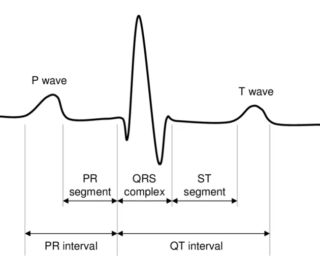
the body and we obtain ECG, and in ideal acquisition conditions we can extract some important parts: the P, Q, R, S and T waves, each corresponding to a single heartbeat as can be seen in Fig.2.2(Seeley et al.,1991).
2.2
Acquisition
As mentioned before, to study the signal we need strategies to collect the ECG from the patient. In this section, we will cover the standard medical acquisition and the acquisition to biometric recognition.
2.2.1 Standard Medical Acquisition
2.2.1.1 12-Lead Configuration
We can consider the heart as a dipole set up in the middle of a sphere constituted by the human body, where the arms and the left leg are approximated to the vertices of an equilateral triangle. As such, the vectors of electric conduction also form an equilateral triangle (see Fig.2.3). Thus, the tensions measured in each derivation are proportional to the projections of the electric vector
6 Electrocardiographic Signal Characterization
Figure 2.3: Einthoven Triangle1.
of the heart on each side of the triangle (see Eq.2.1) (Lin and Sriyudthsak,2016) (Bronzino and Company,2000).
Wilson proposed a way to make unipolar measurements of potential. Ideally, these would be measured against an infinite reference. Thus, the central terminal consists of connecting leads through the same resistor value to a common node. The voltage at this Wilson central node cor-responds to the mean of the voltages in each branch. Normally, 5 MΩ resistors are used, but the higher the value of the resistors, lower the common-mode and the sizes of artifacts introduced, by the electrode-skin impedance. Thus, it is seen that the central terminal of Wilson is in the center of the triangle of Einthoven (see Fig.2.3).
We can modify the leads for increased leads if we remove the link between the member to be measured and the center terminal, which results in a 50% signal amplitude increase. These leads are known as aVL, aVR, and aVF. In addition, 6 leads were introduced to measure potentials near the heart, making a total of 12 leads (see Fig.2.4). They are grouped into three categories: six monopolar precordial leads, three monopolar limb leads, and three bipolar limb leads. The limb leads allow us to get signals from the frontal plane and the precordial leads on the axial plane (Bronzino and Company,2000).
V1−V 2 +V 3 = 0 (2.1)
2.2 Acquisition 7
Figure 2.4: 12 Leads Configuration2.
2.2.1.2 Corrected orthogonal configuration (Vectorcardiography Lead System or Frank
VCG systems)
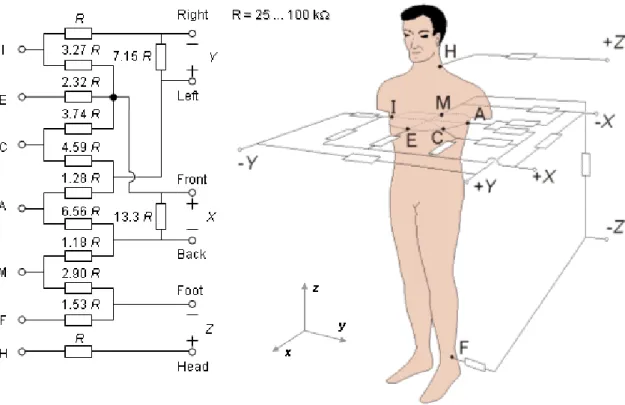
Frank’s lead system was used, in the beginning, for patients in the supine position, with electrodes placed in the fourth intercostal space. Eventually, there was the need to decrease the error due to inter-individual variation (human anatomy), as so it was increased the number of electrodes to seven. It is used scalar leads X, Y, and Z to form the orthogonal lead system. Unlike the 12 leads configuration that uses the frontal and the axis plane (Bronzino and Company,2000).
Normally the electrodes are placed on the chest, specifically on the left (point A), front (point E), right (point I), and back (point M) as it is possible to see in Fig.2.5. Close to the heart (between point A and E), point C is chosen because it is easier to obtain a better signal. In addition, to have a better ground truth and noise removal it is included a point in the neck and one on the left foot (Arrobo et al.,2014).
8 Electrocardiographic Signal Characterization
Figure 2.5: Electrode placement in the Frank VCG system3.
2.2.2 Common ECG Acquisition Settings
2.2.2.1 In-the-Person
Devices in this category are situated inboard the human body. Normally are used only in clinical scenarios to monitor medical conditions. The most widely known example is artificial pacemakers (implantable devices), used to compensate the malfunction of the heart electrical system (da Silva et al.,2015) (Merone et al.,2017).
2.2.2.2 On-the-Person
Nowadays, on-the-person approaches to ECG measurement are the most common, where the sig-nal is obtained through body surface electrodes with the help of a device. This group of devices includes the 12 leads measurement and Frank VCG. With the evolution of technology, it is possible to measure the ECG with wearable devices, like VitalJacket from BioDevices. These approaches have also been commonly used in ECG biometric systems (da Silva et al.,2015) (Merone et al.,
2017) (Cunha et al.,2010).
2.2.2.3 Off-the-Person
In this approach, the sensors are commonly small metallic electrodes to hold in the fingers with the goal of integrating into objects of the daily routine. Here, the user must wear the sensor or
2.2 Acquisition 9
enter voluntarily in physical contact with the sensor. In order to perform ECG acquisition easier through the hand palms or fingers da Silva et al. (2015) proposed a bipolar sensor with virtual ground and dry electrodes. Off-the-person approach allows measuring the ECG at distances of 1 cm even with clothing between the body and the sensor (da Silva et al., 2013) (Bor-Shyh Lin et al.,2013). Another examples is the steering wheel from CardioId4. Although they are used in biometric systems, it is revealed to be a hard task to remove noise.
2.2.3 Variability
In the previous subsection, we detect several factors like an electrical current which makes hard to obtain good results. In consequence of that, the final signal is perturbed.
There may be a lot of possible contamination, in the moment of the signal acquisition and that can contribute to a higher degree of variability. Also, asLabati et al.(2014) shows even in a good acquisition and in normal conditions the subject can have a high variability known as intrasubject variability in only 24h (Pummer,2016) (Schijvenaars,2000).
Several interfering factors exist and can influence the variability on a short-term (ST) or long-term (LT). They can be divided into five categories: environmental factors (LT), lifestyle fac-tors (ST and LT), physiological and pathological facfac-tors (ST and LT), non modifiable facfac-tors and effects and electrode characteristics and placement (ST) (Fatisson et al.,2016) (Schijvenaars,
2000) (Pummer,2016).
Physiological and pathological factors also contribute to variability, such as endocrine factors, respiratory factors, neurological factors, cardiovascular diseases, stress, depression as it is dis-cussed byFatisson et al.(2016). Others factors like body temperature and lifestyle factors such
as physical activity, alcohol, tobacco, drug dconsumption, and meditation are discussed byvan
Ravenswaaij-Arts et al.(1993) andFatisson et al.(2016). Environmental factors like electromag-netic fields, vibrating tools, fatigue also affect variability (Schijvenaars,2000) .
As discussed in the literature (van Ravenswaaij-Arts et al.,1993) (Fatisson et al.,2016) (Labati et al.,2014), in biometric systems the objective is to decrease the intra-variability (the variations between heartbeats of the same person) and increase the inter-variability (the variations between heartbeats of different subjects) of the signals.
2.2.4 Noise Contamination
Besides the variability factors discussed above, the signal can also be contaminated and destabi-lized by noise. The higher amplitude of the heartbeat is in the QRS complex and is between 2-3 mV, so is very common to have a lot of noise in the signal.
Signal noise can have multiple sources, like:
• Baseline wander and motion artifact: Usually result of the subject movements. The base-line wander is caused by breathing movements (involuntary). The motion artifact is commonly associated with random limb movements (Singh et al.,2015).
10 Electrocardiographic Signal Characterization
• Powerline interference: Caused by variation in the electrode impedances and to stray currents through the patient and the cables. It is necessary to remove the AC component, equivalent to the noise of high frequency (consists of 50/60 Hz AC) (Singh et al.,2015) (Levkov et al.,2005).
• Muscle Contraction: Since we are measuring electrical signals and some of the involuntary muscles like the heart contract, electric impulses are generated. When detecting the ECG, it is possible to obtain the signal from the contraction of other muscles.
• Electromagnetic noise: It is induced by the surrounding electronic equipment. The protec-tion circuit limits the maximum voltage that can enter the amplifier to minimize saturaprotec-tion and protect the system. It can be reduced by using magnetic shielding (difficult) or by winding the wires to decrease the area of the loop (Bronzino and Company,2000) (Singh et al.,2015).
• Electrode movement/contact loss: Since the electrodes are in contact with the skin can cause skin irritation. Skin-electrode impedance is very important and can deteriorate the signal (Taji et al.,2014).
• Misplaced Lead: If put the lead in a wrong position that creates electrode contact noise, the ECG will be affected by a frequency of 60Hz (Taji et al.,2014) (Singh et al.,2015).
• Pacemaker interference: Like another device, the artificial pacemakers can interfere in ECG signal captured (Singh et al.,2015).
• Ground Loops: When two machines are attached to the patient, there are two grounds. This may lead to slightly different stresses, creating a current passing through the patient producing a common mode voltage on the electrocardiograph. Aside from being a safety issue, it can raise the potential of the patient (Cutmore,1999).
Since biometrics requires off-the-person measures and as mentioned before in subsection 2.2.2.3, the noise comes up naturally because the environment is less controlled. That can lead to a high signal to noise ratio.
2.2.5 Right Leg Drive
In most modern electrocardiographs, the patient is not connected to ground. Instead, the right leg electrode is connected to the output of an auxiliary operational amplifier. The common mode voltage is felt by two resistors and the signal is inverted, amplified and routed back to the leg. This negative feedback allows decreasing the common-mode voltage, which reduces interference on the electrocardiograph. It can also provide some electrical safety. If any unusual high voltage appears, the auxiliary operational amplifier saturates, and the patient is "disconnected" from the ground because the amplifier can no longer consume for the right leg, and there is no current passing, protecting it (Bronzino and Company,2000) (Kesto,2013).
Wang et al.(2011) applied the right leg drive to the signal in order to reduce common mode noise, allowing to improve the quality of the signal.
In the literature in ECG-based biometric recognition, in the off-the-person acquisition nor-mally the right leg drive is not applied.
2.3 Biometrics Application: Challenges and Opportunity 11
2.3
Biometrics Application: Challenges and Opportunity
At this point, we are aware that electrocardiogram measurement depends on many factors. During this dissertation will be used on-the-person data. Future approaches intended to use off-the-person that increase the challenges in ECG biometric systems.
A biometric system needs to be effortless for the user. That provides sustainable to the off-the-person acquisition, but the obstacles like variability and noise described before can difficult the task.
Since the electrocardiogram is a continuous and cyclic signal we will cover the continuous ECG-based biometric recognition, especially techniques of template update will be studied. In the next chapter, the fundamentals of machine learning are presented.
Chapter 3
Machine Learning: Fundamental
Concepts
3.1
Introduction
Machine Learning (ML) is a field of artificial intelligence that learn from given data in order to recognize patterns. Aims in predict a variable Y from features extracted from data, X , through a function.
In this chapter, the basics of machine learning will be presented including supervised, unsu-pervised and reinforcement learning, feature extraction, dimensionality reduction, classification and performance evaluation.
3.2
Supervised vs Unsupervised vs Reinforcement Learning
One of the tasks in machine learning is supervised learning, where the training data comprises the input vector together with target vectors. A classification problem happens when the target vector is a set of a finite number of discrete categories. We call regression when the output is one or more continuous variables (Bishop,2006).
Another task in machine learning is unsupervised learning, where we do not have targets. The system learns with unlabelled data, identifies likeness data and decide based on the presence or absence of the similarity in each new piece of data (clustering, groups with similar data). We can estimate the data distribution or design the multidimensional data in 2D and 3D for visualiza-tion (Bishop,2006).
Finally, reinforcement learning correspond to an attempt by the agent of approximate to the environment’s function (see Fig. 3.1), such that we can send actions into a black-box that stays in the environment that maximize the rewards it split out, the agents learns from the suc-cess/mistakes (Kaelbling et al.,1996). Some of the basic concepts are described below:
14 Machine Learning: Fundamental Concepts
Figure 3.1: Basic modules of reinforcement learning.
• Agent: In this context corresponds to the algorithm and takes several actions (set of possibles moves that the agent can do) according to the policy established (defines the behaviour of the agent). Does not know the function of the environment (Kaelbling et al.,1996).
• Environment: Corresponds to the surrounding world where the agents take actions. The functions are what transform an action taken in the current state (the immediate situation that the agent finds itself) into the next state and a reward (feedback that allows us to measure the success or failure of an agent’s action, it can be immediate or delayed) (Kaelbling et al.,1996).
• Discount factor: Correspond to a factor that converts future rewards worth less than imme-diate rewards. (Kaelbling et al.,1996).
3.3
Feature Extraction
One of the main steps in machine learning is the feature engineering (begins with a piece of in-formative data and will organize them) because is with these that all the system will work. We can consider feature extraction a dimensionality reduction process (will be explained forward)
because we will reduce the data in a more manageable group also known as feature set (Guyon,
2006). As mentioned byGuyon(2006), the pre-processing transformations may include: normal-ization, signal enhancement, extraction of local features, standardnormal-ization, linear and non-linear space embedding methods, non-linear expansions and feature discretization.
3.4 Dimensionality Reduction 15
3.3.1 Feature Extraction in ECG Biometric
In ECG biometrics, the feature extraction approaches are generally grouped into two categories: fiducialand non-fiducial. Fiducial approaches are very commonly used in biometric systems that make an on-the-person signal acquisition. Fiducial points are landmarks on the ECG complex such as the baseline (PQ junction), and the onset of individual waves such as PQRST. Normally the P wave, QRS complex and T wave are find out and from them are extracted several features as can be seen in Fig.3.2. That means that fiducial point-based methods need the precise boundaries of the waveforms (Plataniotis et al.,2006) (Israel et al.,2005) (Biel et al.,2001).
The most common features described in the literature are:
• The amount of elapsed time between events such as P duration (time of P wave), ST duration (time from S wave until T wave), QT duration (time from Q wave until T wave), QS duration (time from Q wave until S wave), QRS duration (time of the complex QRS), PQ interval (time from P wave until Q wave), RS interval (time from R wave until S wave), PT interval (time from P wave until T wave), RT interval (time from R wave until T wave);
• The maximum distance measured from a position of a vibration or oscillation, such as RS amplitude (distance from R wave until S wave), ST amplitude (distance from S wave until T wave), QR amplitude (distance from Q wave until R wave);
• The inclination of the segments such as RS slope (inclination between R wave until T wave), ST slope (inclination between S wave until T wave);
• QRS onset that correspond to the start point of the QRS wave.
Since biometric research started using off-the-person acquisitions, the signal quality is worse. That difficult the extraction of fiducial features and lead to a new methodology: Non-fiducial approach. Instead of extracting the individual ECG pulses, these methods consider an arbitrary window (example 5 seconds) of the Biometric trait. This kind of approach has a condition, com-monly the window size are bigger than one single heart beat (Plataniotis et al.,2006) (Jung and
Lee,2017). The common methods are Autocorrelation (ACL), Discrete Cosine Transform (DCT)
and Continuous Wavelet Transform (CWT).
The fiducial approach has best results in biometric systems but requires the morphological features capture of the ECG signals. The biometric system complexity increase with these features and need a medical acquisition to have a clean signal to be possible to identify all the fiducials. The non-fiducial approaches have been studied to overcome the disadvantages of fiducial methods. The biggest advantages are no need for synchronization of the heartbeat pulse, and no need of exact heart rate detection, since it differs on each record data and also varies over time (Plataniotis et al.,
2006) (Jung and Lee,2017) (Tan and Perkowski,2017).
3.4
Dimensionality Reduction
After feature extraction, the number of features can become too high for a time-efficient recogni-tion, because it demands a large amount of memory and computation power, or it can ease overfit.
16 Machine Learning: Fundamental Concepts
Figure 3.2: Some of the most common fiducial features extracted in ECG biometrics.
Dimensionality reduction is used to keep the features with the maximum discriminant power and reduce the computational cost for the purpose of improve the performance. Also, can be useful for outlier removal since reduce some features that can contain out range values. Every feature selection method follows these characteristics: research direction, research strategy, evaluation strategy, selection criterion and stopping criterion (el Ouardighi et al.,2007).
Several methods exist such as:
• ANOVA: The one-way analysis of variance is normally applied to determine differences between two or more independent groups, through statistics. The selection of features is performed according to the highest scores (Lee et al.,2013).
• RFECV: The recursive feature selection cross validation determine in each iteration, the worst N features, eliminating them. The remaining features that gives the maximum score on the validation data, is considered to be an optimal number of features (Yeoh et al.,2017).
• SFS: Sequential forward selection is an iterative algorithm that starts with the best individual feature, and adds, at each iteration to the selected subset, the feature that maximizes the criterion function (Zhang and Jain,2004).
• CFS: Correlation feature selection makes the assessment of subsets of features using a crite-rion function that evaluates the correlation of the features with the classification, yet uncorrelated with each other (Zhang and Jain,2004) (Hira and Gillies,2015).
• PCA: The Principal Component Analysis is a subjective approach for dimensionality reduc-tion because seeks a projecreduc-tion that best represents the data by finding a linear transformareduc-tion that preserves best the data. It is used to emphasize variation and bring out strong patterns in a dataset, removing correlated features (Zhang and Jain,2004).
3.5 Classification Methods 17
• KPCA: The Kernel Principal Component Analysis is an extension of PCA but with kernel methods. Basically finds a hyperplane that divides the points into arbitrary clusters, but while PCA is confined to linear transformations, KPCA can find a non-linear manifold (the data are spread to a upper dimensional feature space) which is non-linearly related to the input space (Widjaja et al.,
2012).
• DCT: The Discrete Cosine Transform is an appropriate and flexible choice for a data com-pression algorithm that eliminates less significant features. This method divides the signal into smaller parts and some of the coefficients are selected to construct significant feature vectors or ECG biometrics recognition (Allen and Belina,1992).
• Wilkes lambda stepwise correlation: It is a particular case of ANOVA and measures the individual discriminative power of the variable and as smaller Wilkes Lambda, is more discrimi-native. (el Ouardighi et al.,2007).
• LDA: The Linear Discriminant Analysis is used when the measurements made on indepen-dent variables for each observation are continuous values. Similar to PCA, but LDA endeavours to model the variation between classes of data, and so it requires prior labelling (which can be a disadvantage) (Song et al.,2010) (Karafiat and Burget,2005).
• HLDA: The Heteroscedastic Linear Discriminant Analysis allows to preserve useful dimen-sions and separate the features vectors that represent individual classes. Differs of LDA because requires the estimation of the covariance matrix for each class (Karafiat and Burget,2005).
• SHLDA: Smoothed HLDA similar to LDA and HLDA. Differs from HLDA only in the estimation of the covariance matrices class. The estimation depends on the smoothing factor that goes in the interval of [0,1] (when it is 0 SHLDA behaves like LDA and when is 1 becomes HLDA) (Karafiat and Burget,2005).
• FLDA: The Fisher Linear Discriminant Analysis evaluates locally the levels on the between-class scatter (interbetween-class) and the within-between-class scatter (intrabetween-class) (Sugiyama,2007).
• GBFS: Greedy Best First Search always selects a state with minimum which heuristic value among all candidates (Heusner et al.,2018).
3.5
Classification Methods
To have a score to classify our system we need a classifier to train our model. Normally we have a train set with several samples, and we divide this train group into two parts: one for training and other for testing. Inside of the learning step, we can have a training set (learn the model) and a validation set (used to tune the model’s hyper-parameters). We also can have cross-validation, that is used when we have a few numbers of samples and a proper validation set does not exist. Here, we take the data and split in K number of folds. In 5-fold cross-validation we train the model in 4 dataset partitions and test in the other. In leave-one-out, we train in N-1 samples and test in the other and repeat the process to each sample (only used if the number of samples is too low) (Costaridou,2005) (Beutel,2000). This technique allows us to have a better understanding of the real performance of the system.
18 Machine Learning: Fundamental Concepts
There are several different classification methods, including:
• Naive Bayes: Having a training set, we model each class distribution through normal dis-tribution. Given a new point, we compared the distance to its distribution with the Mahalanobis distance (Euclidean distance if the matrix was unitary). The nearest distribution is the one that most likely generated the new point, and we assign this class to it (Hastie et al.,2009) (Raschka and Mirjalili,2017).
• Logistic Regression: Is a classifier that generates a coefficient that maximizes the similarity of observing the samples values. Tries to look for the best model that describes the relationship between variables, the outcome (dependent) and the predictor/explanatory (independent). The typically variable hyper-parameter is the cost (James et al.,2013).
• Decision Trees: Is an algorithm created to solve a classification problem, by doing several "questions" regarding the attributes of the test record (Hastie et al.,2009).
• Random Forest: Are an extension of Decision Trees. Creates a forest, a group of several decision trees. Normally, how much more trees in the forest, more robust the classifier looks like. Parameters as depth, maximum number of leaves, maximum leaf nodes can be found in these two algorithms (Hastie et al.,2009).
• Multilayer Perceptron (MLP): Is a class of a feed-forward artificial neural networks, with nodes that use non-linear activation functions. The tunable hyper-parameters chosen are the ac-tivation function, alpha (which is a regularization parameter that penalizes weights with large magnitudes), the hidden layer size and the learning rate (Raschka and Mirjalili,2017).
• Nearest Neighbour: Is a non-parametric method that aims in search similarity on vicinity instances. Does not require a model and uses the data directly for classification. The number of neighbours is the hyper-parameter that need to be choose. Normally is odd to avoid ties (James et al., 2013). The kNN can have several different metrics for classification such as Euclidean,
Cosine, and Mahalanobis distance. For example Guennoun et al.(2009) used the Mahalanobis
distance for matching each heartbeat with the template stored in the system database. According to a threshold, decisions are made.
It’s a method that is simple to implement, "training" is very efficient, adapts well to online learning, robust to noisy data but is sensitive to feature value ranges, the classification can be time-consuming and the memory requirements are high.
• Support Vector Machines (SVM): Performs classification in order to find a linear solution (hyperplane) to separate two classes and maximizes the margin between them. The vectors be-tween them that define the hyperplane are the support vectors. In the case of the problem is not linearly separable we can resort to the kernel trick that consist of a transformation of the problem in a bigger dimension (Raschka and Mirjalili,2017).
• Bootstrap Aggregating: Generates weak classifiers/predictors. To make a decision it is used the aggregated average of weak classifiers. Good to use when we have an unstable classifier prediction like in ECG heartbeats data (a little shift in the training data can lead to a big exchange in the construction of the classifier, which will lead to a change in accuracy) (Louis et al.,2016).
3.6 Performance Evaluation: Basic Metrics 19
Figure 3.3: Example of a confusion matrix for a binary medical classifier
3.6
Performance Evaluation: Basic Metrics
Regarding the performance of the system, we need to use some metrics. To better understand the most relevant error metrics, it is needed to understand the basic ones such as TP (true positive), TN (true negative), FP (false positive), FN (false negative) as can be seen in Fig.3.3 (Sim et al.,
2007) (Costaridou,2005) (Beutel,2000)
• Mean error: When the goal is to estimate the value of some scalar or vector quantity. We can focus on the absolute or relative difference between the calculated result and some independent measure of the true value (see Eq.3.1).
MRE= | measure value − true value |
true value (3.1)
• Accuracy (ACC): Measure the correct decisions made by algorithm (see Eq.3.2). Accuracy
may not be a useful measure in the case where there is a large class skew or in case of detection because in this case did not interest to hit in the negative (eg 99% of accuracy with 98% of negative instances).
Accuracy= T P+ T N
T P+ T N + FP + FN (3.2)
• Sensitivity: Concerns how frequently the algorithm classify positive being the value real and positive (see Eq.3.3). Is also called true positive fraction (TPF) or Recall.
Sensitivity= T P
T P+ FN (3.3)
20 Machine Learning: Fundamental Concepts
values are real negative (see Eq.3.4). False positive fraction (FPF) is the same as(1−speci f icity). All these measures can be stated as a fraction between 0 and 1, or as a percentage between 0 and 100%.
Speci f icity= T N
T N+ FP (3.4)
• Precision: The fraction of detections that are relevant (see Eq.3.5).
P= T P
T P+ FP (3.5)
• F-measure: Match precision and recall. The traditional measure is the F1 measure (see Eq.3.6), where P and R are weighted equally. F2 is also commonly used as a measure (see Eq.3.7), that consider recall weights double comparatively to precision, and F0.5, which precision weights twice as much as the recall.
F1= 2× P × R
P+ R (3.6)
F[ =(1 + [
2)× P × R
R+ P× [2 (3.7)
• ROC-Curve: Can be described as the space of possible tradeoffs between sensitivity and specificity. The ROC curve is commonly plotted (see Fig.3.4) with TPF (Sensitivity) on Y-axis and the FPF (1-specificity) on the X-axis. Afterwards, the algorithm runs with different values for this parameter to obtain several TPF/FPF pairs. The ideal performing point is the upper left corner, with TPF = 1 and FPF = 0.
• AUC: Generally it is used the area under the ROC curve (see Fig3.4) as a efficiency measure for evaluating the quality of the curve (consequently the algorithm that produced the ROC curve). The higher the AUC, the greater the probability of making a appropriate decision. One algorithm is globally better than another algorithm if its ROC curve has a greater AUC. However, since the AUC is an overall measure, it may hide important details.
• Free Response ROC-Curve: It is appropriated for when the target is to identify all positive instances in an image. Correspond to have TPF in one axis and FP/image in another axis (for a given value of TP how much FP exist in mean per image). Increasing the sensitivity it increases the number of FP. It is also used the AUC as metric of evaluation.
• Hausdorff distance: Defined as the maximum of the minimum of two distances between two contours of the same object. It is not a true distance metric because it does not verify the commutative property.
• Bland Altman plot: Also called difference plot, it is used to compare two quantitative mea-surements (two different parameters that measure the same property, should be correlated). It is a method to quantify the similarity between two quantitative measurements by constructing limits of agreement.
• Koppa statistic: Also called Cohen’s Kappa, it evaluates the agreement between observers (the inter-observer agreement). It applies in medicine to give a quantitative measure of agreement
3.7 Conclusion 21
Figure 3.4: ROC curve with AUC in authentication problems, FPF (false positive fraction) and TPF (true positive fraction)
between ratters, such as in physical exam findings, segmentation, pathology grading, among oth-ers. While the Bland-Altman plot compares the agreement on real value measurement, Kappa compares categorical labels (see Eq.3.8). Kappa varies in the interval [-1, +1], where 1 is perfect agreement, 0 corresponds to a selection by chance, and the correspondent negative values reveal less agreement than randomly, i.e, high disagreement between the observers:
K= po− pe
1− pe , (3.8)
where p0 is the probability of full agreement and pe is the expected agreement.
3.7
Conclusion
Every aspect discussed in this chapter is very important in biometrics systems since it requires the extraction of the most important features, selection of the best of them and the choice of the model that adapt better to our data in order to have a higher score.
Machine learning techniques are diverse and each one has specific advantages and can be a powerful tool to biometric systems. In this dissertation, we will often resort to machine learning functions for the classification process.
Chapter 4
Biometric Systems: Basics
4.1
Biometric Modalities
Since the first proposal of a biometric system, some different modalities were proposed over time, with the objective of proving the best methodology to guarantee a unique human identification and authentication. Prabhakar et al.(2003),Jain and Kumar(2012) andDelac and Grgic(2004) have listed the most common biometric modalities, like fingerprint, face recognition, hand geometry, iris, voice, palmprint, signature, hand veins, gait, keystroke, and others less common such as ear shape, odour, DNA. Some of these, are ready to commercialize, like a fingerprint which is a very common method in the last generation of smartphones. However, with the evolution of technology, new techniques of counterfeit are used, and already have some successfully spoofing attacks in this area (Hadid et al.,2015), (Akhtar et al.,2015).
Some fingerprint replica can be made using a mould of silicon, iris can be spoofed using contact lenses, voice can be recorded from a phone, faces can be replicated from a 2D photo, DNA can be stooled (Akhtar et al.,2015).
To avoid this, some new approaches were proposed. These kinds of approaches normally guarantee liveness detection, in order to confer resistance to spoofing methods (assure that is a person who is there and not a mold).
Agrafioti et al.(2012) suggest that some of these vital signals carry information that is unique for each human like the electrocardiogram (ECG), phonocardiogram (PCG), photoplethysmogram (PPG), blood volume pressure (BVP), and heart rate variability (HRV). The ECG biometric furnish inherent liveness detection which has computational benefits. Like other vital signals, the ECG signal is very difficult to collect for spoofing purposes (Eberz et al.,2017a).
Nevertheless, vital signals present some disadvantages, and the most significant is their vari-ability, due to several conditions. One good example of this kind of problems is found in the ECG: it can change in a short period of time as shown byLabati et al.(2014).
Nowadays, another approach that is beginning to be implemented is the hybrid system, which combines biometrics traits with traditional credentials like Multi-biometric Authentication System (Fingerprint + Face + iris + Password) from Raviraj Technologies.
24 Biometric Systems: Basics
The next step consists in combining several biometric systems (multimodal biometric systems) likeBe et al.(2015) who used ECG and fingerprint.
4.2
Qualities of Biometric Modality
In the previous section, several biometric traits were presented. According to Prabhakar et al.
(2003), Jain et al. (2004), Abo-Zahhad et al. (2014) and Delac and Grgic (2004) they need to fulfill these characteristics:
• Universality: Every subject must have the characteristic.
• Distinctiveness: The characteristic of two-subject must be distinct. • Permanence: The characteristic should be sufficiently invariant over time. • Collectability: The characteristic should be quantitatively measurable. • Circumvention: The characteristic should be hard to mimic or counterfeit.
• Measurability: The person needs to feel comfortable when the signal is acquired, that means that needs to be an easy and quick process.
• Performance: Practicable recognition accuracy and speed.
• Acceptability: Indicates how much people are willing to accept the use of a biometric iden-tifier.
These qualities are ideal but not mandatory. In fact, there is no biometric feature that fulfill completely these requirements.
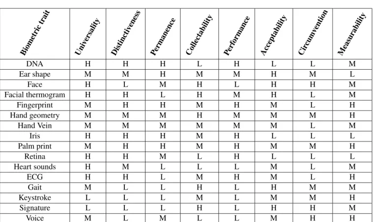
In this work. we will use ECG as a trait, and as we can see through Tab.4.1, it is a trait very balanced.
4.3
Common Structure of a Biometric System:
A biometric system recognizes the individual based on a feature vector derived from their specific characteristic (physiological or behavioural). Basically consist in a pattern recognition system. That feature vector is commonly designated as templates and is usually stored in a database after being extracted as can be seen in Fig.4.1.
4.3.1 System Modules
According toBolle(2011), a simple biometric system hold five basic components (represented in Fig.4.2):
• Sensor Module: Captures the biometric trait data, usually resort to sensors;
• Feature extraction module: Verifies the acquired data and process them to extract feature vectors;
• Matching module: Compares feature vectors against those of the stored templates (from the database);
• Decision-making module: The user’s identity is determined, or verify if a claimed identity is genuine (accepted) or impostor (rejected).
4.3 Common Structure of a Biometric System: 25
Table 4.1: Comparison between biometric traits regarding the seven
char-acteristics (H - high; M - medium; L - low) (based on Prabhakar et al.
(2003),Jain et al.(2004),Abo-Zahhad et al.(2014) andDelac and Grgic
(2004)). Biometric trait Uni versality Distincti veness
Permanence Collectability Perf ormance Acceptability Cir cumv ention Measurability DNA H H H L H L L M Ear shape M M H M M H M L Face H L M H L H H M Facial thermogram H H L H M H L M Fingerprint M H H M H M L H Hand geometry M M M H M M M H Hand Vein M M M M M M L M Iris H H H M H L L L Palm print M H H M H M M H Retina H H M L H L L L Heart sounds H M L L L M L M ECG H H L M H M L H Gait M L L H L H M M Keystroke L L L M L M M H Signature L L L H L H H M Voice M L M L L M H H
26 Biometric Systems: Basics
Figure 4.1: Simplest scheme of biometric for a continuous system that use template update.
• Database module: Stores the biometric data. Also, it can be updated after verification in a continuous biometric system as described byLabati et al.(2013) andSufi and Khalil(2011).
4.3.2 Operation Modes
Two modes of operation exist in Biometric systems: verification (authentication) or identifica-tion. Concerning identification, the acquired biometric information is compared against templates corresponding to the totality of users in the database (one-vs-all problem), verification involves verify the similarity between templates that correspond to the claimed identity (two class prob-lem, one-vs-one comparison). Hereupon, it is implies that we should deal with this two problems (identification and verification) separately.
4.3.3 Conventional vs Continuous Biometrics
Regarding the moments of identification or verification, there are two types of biometric systems. Conventional Biometrics are those that control access to a safe room/system, usually not requir-ing the user to re-authenticate himself for continued access (at least not for a considerable long period of time) to the protected resource, (i.e one-time verification system). In high-security en-vironments, this may not be sufficient because the protected resource needs to be continuously monitored for unauthorized use (Sim et al.,2007) (Niinuma and K. Jain,2010).
To solve this problem, continuous biometrics systems can be used but they are still in de-velopment phase. According toSim et al.(2007) the continuous verification needs to follow six criteria:
1) Reliability: Any continuous system must take into account the trusty of each modality; 2) Template update: Older observations increase uncertainty, so it needs to have low weight when used to verify the legitimate user;
3) Liveness: whether the legitimate user is present or not;
4) Usability: The system must not demand re-authentication when for example the user takes a break to get some air, it needs to be convenient;
4.3 Common Structure of a Biometric System: 27
Figure 4.2: Module representation of the five basic components.
5) Security: If the user get away from the device the system must require active re-authentication; 6) Cost: The system should be design/implemented with commercial purpose (off-the-shelf devices only). Should avoid the use of special/expensive devices.
Since new data is constantly acquired we need to have in mind that not all biometric traits are viable for this process. With this in mind and with the new technologies of ECG signal acquisition (discussed in section2.2.2), we consider that ECG signal is one of the most convincing traits because we can acquire the signal easily and be comfortable for the user.
4.3.3.1 Conventional Biometrics
To apply and predict the potential of a biometric system in a real-life situation, the evaluation of its performance is needed.
Since we are focusing on problems of identification or verification, different metrics must be used (as inRibeiro Pinto et al.(2018),Pinto et al.(2017)). In a biometric system, we can have dif-ferent problems respectively to the subject, the system or database. We can have several difdif-ferent situations regarding a biometric system. The situation where the subject is already registered in the system and the system identifies him correctly (allowing the access). The situation where the subject is register and the system fails in identify him (rejecting the access). Another scenario is when the subject is registered, but the system allows access under the identity of another subject. Other development that can surge in the system is when the subject is not register but can have access because the system misses the identification (identifies the subject as one of the enrolled subjects). At last, we can have a situation where the subject is not enrolled and the access is denied.
According toGrother et al.(2011) exist two types of categories errors:
• Type I: When the system fails to identify the subject (genuine user) with the respectively stored template;
• Type II: When the system matches wrongly the subject with a different person’s stored template (impostors).
28 Biometric Systems: Basics
As mentioned byGrother et al.(2011) our goal is to maximize the situations where the subject is registered and the system identify or not the subject in order to achieve the best performance possible. The solution to guarantee the best performance can be a solid template update method.
4.3.3.2 Identification Error Metrics
Costaridou(2005),Beutel(2000),Grother et al.(2011) andGorodnichy(2009) divide the most relevant metrics in two groups. The first group focuses on situations where the subject being identified is enrolled in the system:
• True Positive Identification Rate (TPIR or Hit Rate or rank-k identification rate): It is the de-sired proportion of identification transactions by users registered in the system, where the subject correct identity is among the R strongest identities returned by the system (see Eq.4.1). The value of TPIR is called rank-one accuracy;
T PIR(R, T, L) =No.of trials where, among L, one of the strongest R predictions above T is correct Total number of trials
(4.1) • Accuracy: It is the correct identification of subject on total samples. When we consider the strongest prediction (R = 1) of TPIR above the threshold T (see Eq. 4.2), it is reached the identification rate. Can also be refereed as IDR;
IDR(T, L) = T PIR(1, T, L) (4.2)
• Reliability: When we choose R = N (number of enrolled subjects)(see Eq.4.3);
Reliability= T PIR(N, T, L) (4.3)
• False-Negative Identification Rate (FNIR): It is the opposite of TPIR, where the test exam-ples are classified as false although they are true (Type 2 error) (see Eq.4.4);
FNIR(R, T, L) = 1− T PIR(R,T,L) (4.4)
• Misidentification Rate: Correspond to the opposite of accuracy, when we measure the frac-tion of total trials where with the subject enrolled in the system, the true identity is not the system’s top ranking prediction above T (see Eq.4.5). Equivalent to FNIR with R = 1;
MIDR(T, L) = 1− IDR(T,L) (4.5)
4.3 Common Structure of a Biometric System: 29
• False Positive Identification Rate (FPIR): Is the ratio where the test examples that are classi-fied as true, although they are false (type 1 error) (see Eq.4.6);
FPIR(T, L) =No. of trials with unenrolled subjects where there us ine or more predictions above T Total number of trials
(4.6) • Selectivity: Provinient of FPIR but here we consider the average number of predictions above the threshold T (see Eq.4.7);
Selectivity(T, L) =No. predictions above T across all trials
Total number of trials (4.7)
• Cumulative Match Characteristic (CMC) curve, plots the rank-k identification rate against k. These rates are not enough for a full picture of the system performance.
4.3.3.3 Verification Error Metrics
As presented in section3.6a system can have two binary errors: FP and FN (Gorodnichy,2009). Using a biometric system on a data set, the total number of FP (also known as False Accept) and FN (also known as False Reject) are find out to compute the cumulative measurement:
• False Accept Rate (FAR): correspond to accept incorrectly an access attempt by an unautho-rized user, as can be seen in Eq.4.8;
• False Reject Rate (FRR): correspond to reject incorrectly an access attempt by an authorized user, as can be seen in Eq.4.9;
With both, we can define a threshold, and we can measure two different metrics:
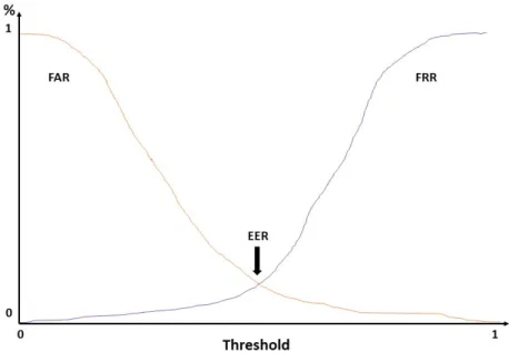
• Decision Error Tradeoff (DET) plot, corresponds to the chart of FAR vs FRR, obtained by changing the system match threshold, and allows us to extract one important measure known as Equal Error Rate (EER) that represents the operation point where FAR = FRR as can be seen in Fig.4.3;
• Receiver Operating Characteristic (ROC) curve that plots TAR against FAR. FAR(T ) = Number of impostor trials where the prediction score is above T
Total number of impostor trials (4.8)
FRR(T ) = Number of legitimate trials where the prediction score is below T
Total number of legitimate trials (4.9)
4.3.4 Continuous Biometrics
In the situation of conventional biometrics (i.e. not continuous, like previously described), metrics like FAR and FRR are sensible and widely accepted metrics. Nevertheless, continuous authenti-cation provides a unique challenge because the system accumulate errors over runtime. Here, we can have two scenarios, one corresponding to the meaning of FAR and the other corresponding to the systematic FN. In the first scenario, a FAR of x% mean that this percentage of invaders never
30 Biometric Systems: Basics
Figure 4.3: DET plot, represented by FAR (curve on green) and FRR (curve on red). EER is the intersection between the curves.
have been detected while all others are exposed immediately. In the other scenario, the systematic FN can be permanent or difficult to remove in the situation where the behaviour of the invader and the user is very similar. From a security point of view, these errors can be problematic, because an unauthorized subject can access the system and compromised it for unlimited time. (Eberz et al.,
2017b).
Here we must consider the difference in the reliability of several modalities. Since the bio-metric trait can change over time, older biobio-metric observations should have less weight to reflect the raised uncertainty of the continued presence of the rightful user with time. Also, the system should determine the authentication certainty in any period, even when no biometrics observations are available for one or more modalities (Niinuma and K. Jain,2010).
Since time is not taken into account in FAR and FRR we can consider obsolete for this kind of system.
InSim et al.(2007) they developed metrics that succinctly capture the global system perfor-mance, allowing to compare different systems.
1) Time to Correct Reject (TCR)→ The authors define as the period between the beginning
of the first action taken by the imposter, to the instant that the system decides to (correctly) reject him (unit is seconds). TCR should be zero (impossible computing) but if TCR fails to correctly reject the imposter, TCR will be infinite;
2) Probability of Time to Correct Reject (PTCR)→ The authors define as the probability that TCR is less than the window of vulnerability (W). Ideally should be 1. The system sometimes can tolerate PTCR less than one to correctly reject an imposter;
4.3 Common Structure of a Biometric System: 31
protected resource. Ideally, Usability should be 1, that means that the legitimate user is granted access all the time;
4) Inconvenience→ The authors define as 1 – Usability. When it denied access to the legiti-mate user, it represents an nuisance to him because he must re-authenticate himself or take other action to restore access;
5) Average Usability→ The authors define as the sum of activity-specific usabilities weighed but with the percentage of time spent on each activity;
6) Usability-Security Characteristic Curve (USC) → Corresponds to the plot Usability vs
PTCR. This is analogue to the ROC-curve in one-time measure verification system. As a per-formance measure it is used the area under USC curve.
4.3.5 Biometric Menagerie
Each person behaves differently regarding biometric authentication systems and each of them is responsible for complicating the task of biometric authentication. In the literature it was formal-ized as the concept of Biometric Menagerie (R. Doddington et al.,1998) (Yager and Dunstone,
2010), (Houmani and Garcia-Salicetti,2016) and (Teli et al., 2011), defining and labelling user groups with animal names to show their characteristics comparatively to biometric systems.
The first timeR. Doddington et al.(1998) created the concept, the authors defined four types of animals that will characterize the system errors. They define the zoo as:
Sheep → The subject produces a biometric template that matches well to other biometrics
templates of themselves and poorly to other people. Exhibit low FRR.
Goats→ The subject produces a biometric template that matches poorly to other biometrics
templates of themselves. Exhibit high FRR.
Lambs→ The biometric template of a subject can easily imitate from a biometric template of a different person. Exhibit the increasing of FAR.
Wolves→ The biometric template of a subject is an amazing impersonation, can imitate the
other person. Exhibit a significant increase of the FAR.
Doddington’s definitions did not capture the relationships between match and non-match scores.
Teli et al.(2011) define a new zoo based on match scores, according to a user’s relationship be-tween the genuine and impostor match scores. They define:
Doves(sub-group of Sheep)→ Match very well against themselves and poorly against others.
Chameleons→ Generally match well with every sample.
Phantoms→ Generally match poorly with every sample.
Worms(sub-group of Goats) → Match poorly with themselves and well with the rest of the
persons.
InYager and Dunstone(2010), the authors have made a study for comparing these two zoos’ and apply this concept in an online signature. InPaone and Flynn(2011), the authors apply these ideas in iris matches for testing the consistency. As Poh et al. (2006) have done, this kind of approach is good for testing to assess user-dependent variabilities.
32 Biometric Systems: Basics
The zoos have in account the difference in the population and allow us to evaluate the distri-bution of people in different categories. That allows a better characterization of the results.
4.3.6 Ideal Conditions for a thorough Performance Assessment
After this review of the most common methodology, we realize that the most important metrics are time-dependency. Also, it is possible to conclude that we need to separate the problem in two big parts and deal with them individually. For identification, the most common metrics are accuracy or Identification Rate. For authentication, they use more FAR, FRR and EER.
Biometric menagerie appears to be influential on the system’s performance, and from the way that we evaluate the system, as previously described.
4.4
System Design Considerations and Concerns
Despite all the concerns referred, when we are designing a new biometric system we need to have in account several aspects, even when we are planning a business case as statedYanushkevich and Shmerko(2009),Wayman(2005).
• One important aspect is the business plan, where it is taken into account, with a high level of detail, the fundamental pieces for the set-up. Since is a biometric system is namely for security purpose and requires time, money and energy for the set-up;
• In real life situation the systems are not successful every time. As such, not all people will be able to use them. This implies that backup systems for exception handling will always be required; • Despite the high level of acceptance of biometric technology will always exist some people that will reject and argue against the technology. Whereby we should study very well the needs of the population;
• Since biometric systems are commonly used for safety/security, the integration of data will be a hard task because all requirements of a biometric system must be attended by hard-ware/software. In order to accomplish that it must be required the authorization by the users to store the data;
• Since we are in an era of quick technology development, the product and the competitors can be in a continuous flow. So the technology that we invest today may not make sense in the next year;
• The addition/substitution of a component will inevitably lead to a change in the business process. This kind of situation must be avoided;
• Intellectual property and approval by the competent authorities are of extreme importance in
order to be able to commercialize the product and protect them (e.g FDA, INFRAMED, CE) (Rossi
4.5 Summary and Conclusions 33
4.5
Summary and Conclusions
The potential of Biometric systems is huge, and clearly brings a lot of advantages comparing to the traditional techniques like ID-cards as we mentioned before. To use biometric identity we require the intrinsic characteristic of the individual and guarantee the relation between the identity and person requesting access.
In this work we will focus on long term Electrocardiogram, to improve these measures and allow future comparison between the several methods (Bolle,2011).
Nowadays, some advanced systems already use biometric modalities like face and fingerprints but as we said in this chapter, this can be manipulated and can be copied. Electrocardiogram appears as one of the best biometrics modalities because of his advantages.
However, in the recent studies, the ECG advantages did not translate in accuracy when we talk about continuous measures and that give us a space to improve this system.