ELECTROTECHNICS, ELECTRONICS, AUTOMATIC CONTROL, INFORMATICS
This paper was recommended for publication by Emil Rosu 11
ESTIMATION OF STEEL SOLIDIFIED LAYER THICKNESS, FOR CONTINUOUS CASTING CONTROL PURPOSES
Mihai MUNTEANU, Emil CEANGA
“Dunarea de Jos” Galati University, Control Systems and Industrial Informatics Department Domneasca – 47, Galati – 800008, Romania
E-mails: [email protected], [email protected]
Abstract: An important goal in continuous casting automation process rest in establishing a proper casting speed being able to assure a compromise between machine productivity and solidified skin cracking protection on the mould level. Contextually, this paper presents new solutions regarding solidified layer thickness estimation for steel continuous casting. The new model starts from actual stadium analysis and propose a solution for analytical model modification, in such a way that the model to approximate solidification dynamics at different casting speeds, using both important parameters for continuous casting process, meaning casting speed and time. A series of results obtained using numeric simulation are presented as a validation for proposed solution.
Keywords: continuous casting, layer solidified thickness, mathematical modeling, automatic control.
1. INTRODUCTION
Continuous casting process is one of the most important processes in the steel production industry and consists in transformation of steel aggregation status from molten to solid. A fully and comprehensive description of these processes can be found in (Oprea, F., et al, 1994).
Automation control for continuous casting machine is a very complex problem and involve development of adequate mathematical models (Thomas, B.G., 2001), (De Keyser, R., 1977), X. (Huang, X., et al.
1992), (Simon F, et al,1997).
An important goal in continuous casting automation process is represented by steel layer solidification thickness obtained at the exit from mould. This solid steel layer thickness must have enough width to support the mechanical efforts which are applied to the strand in the following production steps. To achieve this is necessary to establish an estimation
solution using models for solid steel thickness at the mould exit, as base for process automation, known that there is no method for direct measurement of this thickness. Research in this field was published by (Thomas,B.G., 2001). In essence, there are monitored cases when solidified thickness layer at the exit from the mould is thin and possibility of cracking is real. These situations occurred mainly in dynamic regime caused by set point changing (casting speed modification) but also due to bad operation with the whole machine.
To solve this problem a series of solutions were generated, materialized in two types of models:
− analytical model, resulted from applying of idealized boundary conditions and
12 Both methods presents important inconvenient due to approximation involved. A series of proposal for reducing these errors induced by these approximations are presented in (Barbu, B., et al
2002); Barbu, B. , et al, 2003). Present paper proposes a new method for steel solidified layer thickness estimation, which allows approximation for solidification dynamics on different casting speeds. Paper is organized in the following manner: in next two sections are presented analytical model and Hills model including modifications proposed in (Barbu,
B., et al, 2002; Barbu, B., et al, 2003). Section 4
contains corrected model proposed in this paper and in section 5 are presented results obtained by numerical simulation, which shown the properties of proposed model. One conclusions section ends the paper.
2. ANALYTICAL MODEL
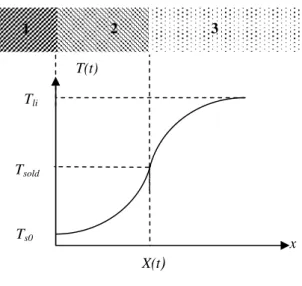
For solidification process on the mould level is considered a molten with uniform initial temperature, considered known, Tli. In initial moment, t=0,
temperature at coordinate x=0 is reduced to Ts0 value,
below the solidification temperature, Tsold, due to heat
transfer from steel to mould wall. At a certain moment t, temperature distribution becomes shaped as is presented in fig. 1 and solidified layer has thickness X(t).
Due to the fact that solidified thickness is reduced on the mould level comparing with molten thickness non-permanent regime, can be considered, as hypothesis, that molten steel medium is semi-infinite (for x>X(t)). Unidirectional heat transfer is described by two equations corresponding both solid state and molten state.
For solidified layer, status equation is: (1)
2
2
s s
s
T T
t α x
∂ ∂
=
∂ ∂ for 0 ≤
x≤X(t)
where αs is thermal diffusivity for solid steel.
For molten layer, status equation is similar: (2)
2
2
l l
l
T T
t α x
∂ ∂
=
∂ ∂ for
X(t)≤x < ∞
where αl is thermal diffusivity for molten steel.
Equations (1) and (2) have the following limitation conditions:
(3)Ts(x)|x=0 = Ts0 ; t>0
(4)Tl(x)|x→∞ = Tli ; t>0
Limitation condition related to solid-molten interface is:
(5)Tl = Ts = Tsold at x=X(t)
Initial conditions are:
(6)Ts(x)|x=0, t=0 = Ts0 ; Tl(x)|x>0, t=0 = Tli ;
In order to calculate solidification boundary speed, will be used energetic equilibrium equation in metal.
(7) heat generated absolute heat flow
solidification derivate = at molten- solid interface
Heat generated per volume, due to solidification, is
s H, where s is solid phase density and H is latent
solidification heat. In these conditions energetic equilibrium equation in metal is:
(8) S. H.dX t( ) l. Tl S. TS
dt x x
ρ ∆ =λ ∂ −λ ∂
∂ ∂
where l and s are thermal conductibility coefficients for both solid phase and molten phase. According with the previous, process model for primary cooling will consist in:
Initial data: physical and material constants: αs, αl,
Tsold, l, s, ρs, ∆H, mould length.
Measured variables: Ts0 (mould temperature), Tli
(tundish current measured steel temperature). Mathematical model:
2
2
s s
s
T T
t α x
∂ ∂
=
∂ ∂
2
2
l l
l
T T
t α x
∂ ∂
=
∂ ∂
Ts(x)|x=0 = Ts0 ; Tl(x)|x→∞ = Tli
Tl = Ts = Tsold
Ts(x)|x=0, t=0 = Ts0 ; Tl(x)|x>0, t=0 = Tli
X(t
)
x Ts0
Tsold
Tli
T(t)
1 2 3
Fig. 1 Temperature distribution in mould solidification. 1. water cooled mould;
13
( ) l S
S l S
T T
dX t H
dt x x
ρ ∆ =λ ∂ −λ ∂
∂ ∂
Output variables: solidified layer thickness at the
mould exit/ solidification boundary speed.
Analytic solutions for this mathematical model conduct to a solidification boundary dynamic having the following form
(9)X t( )=2.K . αs.t
where calculation method for K coefficient is presented in (Oprea,F., et al.1994). Analytical solution (9) generates an overestimation for solidified layer thickness, which is unacceptable. A series of modifications for this model were accomplished by (Barbu, M., et al, 2002; Barbu, M., et al, 2003) in order to obtain a model improvement. The model proposed in these papers contains two exponential correction terms which becomes zero very fast with time incrementation. Relation for solidified layer thickness becomes:
(10)X t( )=2.K .( αs. q .( exp(−q .t1 )+t)− αs.q .exp(−q .t1 ) )
where q=4.2; q1=0.013. 3. HILLS MODEL
A different model used for solidification process on the mould level is Hills model (Thomas,B.G., 2001) for which explanation, Hills hypothesis will be adopted as follows:
I1 – molten steel is homogenous from thermal point of view so no thermal gradient in molten will be considered;
I2 – heat transfer by thermal conductibility is ignorable in strand movement direction and is considered only in rectangular direction regarding mould wall;
I3 – thermal transfer coefficient between outer solidified surface and mould wall is considered known and constant on y strand moving direction. Using these hypotheses thermal transfer model through convection in solidified layer can be written:
(11)
2
2
. .
s s s
s t
T T T
V
t α x y
∂ ∂ ∂
= =
∂ ∂ ∂ , 0≤x≤ X y( )
where Vt dy dt
= represents casting speed; X y( ) is
solidified layer thickness at y distance from upper surface of the mould.
Condition for solidified layer limitation is:
(12)Ts =Tsold at x=X y( )
Thermal equilibrium equation at solid molten interface is:
(13) .S s . T. ( ). t
T dX y
H V
x dy
λ ∂ ρ
− = ∆
∂ ,
x
=
X y
( )
where
∆
H
t is solidification heat plus heat overplus due to the fact that molten steel temperature is superior toT
sold:(14)∆HT = ∆Hs+Cps.(Tsold −Tli)
Boundary condition on x=0, to wit on contact between solidified outer surface and mould wall is:
(15) s. s c.( s c)
T
h T T
x
λ ∂ = −
∂ at x=0
where Tc is mould wall temperature, hc thermal transfer constant between solidified outer layer and mould wall.
Equations (11) – (15) forms based model from which Hills calculated solution for solidified layer thickness at the mould exit is obtained. According with this solution a series of constants are defined as follows:
- dimensionless distance on movement direction:
(16)
2
.
. .
.
c
t ps s
y h
V
C
ς
ρ
λ
=
- dimensionless thickness for solidified layer:
(17) c
. ( )
s
h X y
X
λ
=
- latency heat plus dimensionless overheating: (18)
.
T Tps sold
H
H
C
T
∆
∆
= −
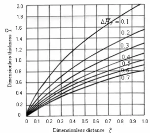
Hills solution for (11) – (15) equations model is materialized in function:
(19)
X
=
F
( ,
ς
∆
H
T)
14 Fig. 2 Dependence between dimensionless thickness
and dimensionless distance (Oprea, F., et al, 1994) 4. CORECTED ANALYTICAL MODEL The following preliminary conclusions were generated analyzing presented methods:
1. analytical model conducts on a
( )=
X t K . t relation, which is considered as a
classical model in solidification processes. Anyway, this analytical model is based on nonrealistic boundary first order condition. Even in this hypothesis Ts(x)|x=0=Ts0 temperature is non
measurable (is known with a very high level of imprecision);
2. analytical model describes solidification process dynamics not using casting speed as independent input variable;
3. Hills model uses realistic second order boundary conditions, but thermal coefficient transfer between outer solidified layer and mould wall, hc, can be evaluated with a very high level of imprecision, due to complex structure (and unpredictable) of contact between solidification skin and mould wall.
4. Hills model includes casting speed as independent input variable but there is no explicit dependence between t and solidified layer thickness. In dimensionless form the model is used for obtaining solidified layer thickness in stationary regime.
Considering all these aspects is proposed a much simple solution for analytic model, in such a way that to obtain an approximate solidification dynamics on different casting speeds. Information provided by this model is used in primary cooling monitoring and refers to an estimation of solidified layer thickness. From safety reasons it was considered that estimated thickness must be smaller than the one obtained from Hills model.
Solidified layer thickness depends upon two independent variables: casting speed and tundish steel temperature. Correction takes into consideration differences between two previous models, to wit:
- Analytical model (which will be corrected), with boundary first order conditions;
- Hills model (the one used by operators in permanent regime), with boundary second order conditions.
Faster solidification dynamics of analytical model is determined by the fact that Ts(x)|x=0=Ts0 temperature,
considered known in analytical model has a direct influence – by system status equations – on temperature spatial distribution. In case of second order boundary condition, thermal flow modification
. s .( )
s c s c
T
h T T
x
λ ∂ = −
∂ on outer solidified layer determines through a dynamic process Ts(x)|x=0=Ts0
temperature. This temperature dynamics is slower than thermal flow dynamics. In these conditions changing in analytical model structure must include also a dynamic subsystem, having parameters dependant upon casting speed so that, solidified layer thickness modification speed to be approximately equal with the one generated by Hills model. Basic diagram for this correction is given in Fig. 3.
Dynamic subsystem model using for analytical model solution filtration is a second order model and has parameters dependant upon casting speed:
Xc1(k)=aXc1(k-1)+(1-a)X(k);
Xc(k)=(a+d)Xc(k-1)+(b-c.vt(k))Xc1(k);
where k is discrete current time, vt(k) represents
casting speed, and subsystem parameters are:
a = 0.65; b = 0.475, c = 25 and d = 3.
0 20
40 60
80
2 4 6 8 10
x 10-3 0 0.01 0.02 0.03 0.04 0.05
X(t)
vt
t
a
Ts0
Analytical model
Tli X t( )=2.K . αs.t
Dynamic subsystem
Xc(t,vt)
vt
15
0 20
40 60
80
2 4 6 8 10
x 10-3 0 0.01 0.02 0.03 0.04 0.05
X(t)
t vt
b
0 20
40 60
80
2 4 6 8 10
x 10-3 0 0.01 0.02 0.03 0.04 0.05
X(t)
t vt
c
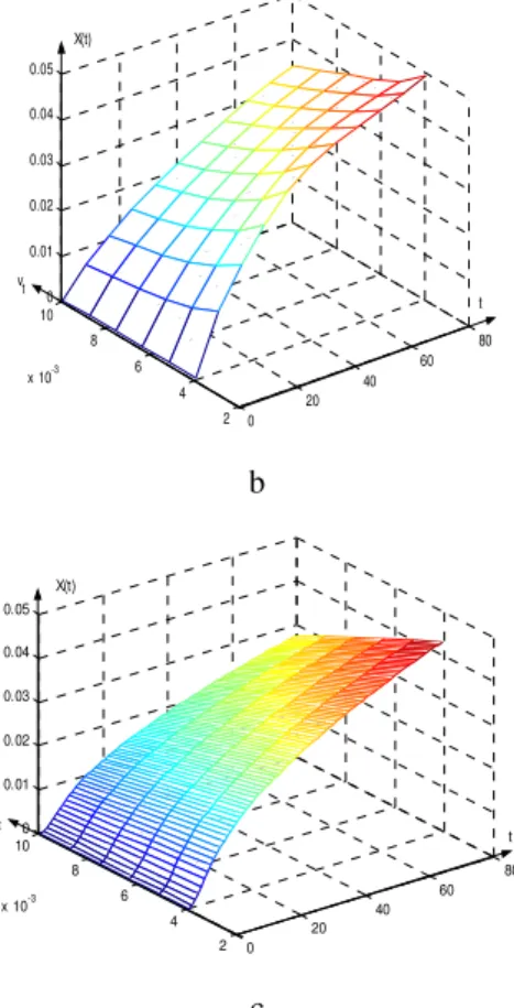
Fig. 4 Solidified skin dynamics on different casting speeds: (a) –analytical model case; (b) – Hills model case; (c) – analytical model corrected case 5. RESULTS OBTAINED USING NUMERICAL
SIMULATION
In Fig. 4 is presented the dynamics of solidified skin on different casting speeds in the following conditions:
– Analytical model case (Fig. 4.a), when casting speed did not influence the dynamics of solidified skin;
– Hills model case (Fig. 4.b);
– Analytical model corrected case (Fig. 4.c). In analytical model corrected case, the solidification layer thickness evolution is similar with situation generated by Hills model. For an easier comparing in Fig. 5 are displayed solidification layer thickness estimation based upon Hills model (dashed line) and based upon corrected analytical model (solid line) for different casting speeds. It was considered useful that on high casting speeds and on relatively higher time values (t > 50s), when position of solidified layer corresponding with exit mould zone, estimation obtained from corrected analytical model to be inferior to the one gave by Hills model. This estimation is useful for achieving protection functionalities; in this context a reasonable negative tolerance is recommended.
As it was mentioned also in fig. 3, solidification layer thickness estimation is influenced by Ts0 temperature
and molten steel temperature measured in the tundish, Tli. Considering uncertainties in obtaining
these parameters, it was analyzed the impact of them in X(t) estimation.
0 10 20 30 40 50 60 70 80
0 0.005 0.01 0.015 0.02 0.025 0.03 0.035 0.04 0.045 0.05
6 5 4
3 2 1 1 - v
t = 0.01 m/s 2 - v
t = 0.0088 m/s 3 - v
t = 0.0076 m/s 4 - vt = 0.0064 m/s 5 - v
t = 0.0052 m/s 6 - v
t = 0.0040 m/s X(t)
t
Fig. 5 Solidified layer thickness estimation, on different casting speeds, obtained from Hills model (dashed line) and from corrected analytical model (solid line)
In Fig. 6 are plotted the evolution of X(t) thickness estimation, on Ts0 temperature equals with: 400K, 450K, 500K and 550K, both in corrected analytical model (I curve), and in analytical model (II curve). In this case, is easier to observe that, effect of Ts0
temperature variation is reduced. Also usual variations for tundish molten steel temperature over solidification rate are reduced, as can be observed in Fig. 6. In this picture are plotted also with dashed line, results obtained with Hills model.
0 10 20 30 40 50 60 70 80 0
0.005 0.01 0.015 0.02 0.025 0.03 0.035 0.04 0.045 0.05
1 2 3 4
1 2 3 4 1 - T
s0 = 400K 2 - T
s0 = 450K 3 - T
s0 = 500K 4 - T
s0 = 550K X(t)
t (II)
(I)
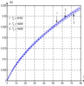
16
0 10 20 30 40 50 60 70 80
0 0.005 0.01 0.015 0.02 0.025 0.03 0.035
X(t)
t 1
2
3 1 - Tli = 1810K
2 - Tli = 1825K 3 - Tli = 1840K
Fig. 7 Tli temperature influence on X(t) thickness evolution
6. CONCLUSIONS
Results plotted in fig. 6 and 7 states that are possible to work with values considered “rated”, constants, for
Ts0 and Tli temperatures. Anyway, Tlitemperature can
be calculated with enough precision from global model for ladle-tundish assembly. This model is initialized using effective measured temperature of molten steel in the tundish (this temperature is measured 4 times per heat in tundish). Also mould wall temperature is measured constantly during the heat in such a way that temperature Ts0 variations can be considered approximately as variations of measured temperatures.
Concluding, even if solidified model sensibilities in relation to Ts0 and Tli variables are reduced,
automation system can use data from measurements and from ladle-tundish assembly model in order to obtain reducing estimation error.
7. REFERENCES
Barbu, M, Ceanga, E, Gheorghiu, C (2003), Real Time Supervising Modeling of a Continuous Casting Mold Using Artificial Intelligence
Techniques, 11th Mediterranean Conference on
Control and Automation - MED2003, Rhodes, Greece, Proceedings CD-ROM, June 18-20. Barbu, M, Gheorghiu, C, Ceanga, E. (2002), Model
matematic pentru supervizarea in timp real a regimului de racire primara la instalatiile de
turnare continua a otelului, a XII-a Conferinta
Nationala de Termotehnica, cu participare internationala, Proceedings CD-ROM, Pag. 159-170, ISBN 973-8303-16-9, Constanta, Romania, 14-16 Noiembrie.
De Keyser, R. (1977) Model Adaptation for Predictive Control in a Continuous Steel Casting Line, IFAC ADCHEM, Banff, Canada.
Mattsson S. (1997), On modeling of heat exchangers
in modelica, Proceedings of the 9th European
Simulation Symposium, ESS'97, Oct 19-23, 1997, Passau, Germany
Oprea, F. s.a. (1994), Teoria proceselor metalurgice, Ed. Didactica si Pedagogica, Bucuresti.
Simon, F, Bernhard, S, Rake, H. Gain (1997)
Scheduling PI-Control of Strip Casting Plant,
Poc. of the IFAC-IFIP-IMACS Conference, Belfort, France, 20-22 May
Thomas,B.G. (2001) Continuous Casting: Modeling,
The Encyclopedia of Advanced Materials,
Pergamon Elsevier Science Ltd., Oxford, Vol. 2. X. Huang,, B. G. Thomas, et al. (1992), Modeling
Superheat Removal during Continuous Casting