An empirical model simulating long-term diurnal CO<sub>2</sub> flux for diverse vegetation types

(1)

BGD

5, 4001–4034, 2008

An empirical model simulating long-term

diurnal CO₂flux

M. Saito et al.

Title Page

Abstract Introduction

Conclusions References

Tables Figures

◭ ◮

Back Close

Full Screen / Esc

Printer-friendly Version

Interactive Discussion

Biogeosciences Discuss., 5, 4001–4034, 2008 www.biogeosciences-discuss.net/5/4001/2008/ © Author(s) 2008. This work is distributed under the Creative Commons Attribution 3.0 License.

Biogeosciences Discussions

Biogeosciences Discussionsis the access reviewed discussion forum ofBiogeosciences

An empirical model simulating long-term

diurnal CO

₂

flux for diverse vegetation

types

M. Saito1, S. Maksyutov1, R. Hirata2, and A. D. Richardson3

1

Center for Global Environmental Research, National Institute for Environmental Studies, Tsukuba 305-8506, Japan

2

National Institute for Agro-Environmental Sciences, Tsukuba 305-8604, Japan

3

Complex Systems Research Center, University of New Hampshire, Durham, NH 03824, USA Received: 27 August 2008 – Accepted: 27 August 2008 – Published: 9 October 2008

Correspondence to: M. Saito (saito.makoto@nies.go.jp)

(2)

BGD

5, 4001–4034, 2008

M. Saito et al.

Title Page

Tables Figures

◭ ◮

Back Close

Full Screen / Esc

Abstract

We present an empirical model for the estimation of diurnal variability in net ecosystem CO2exchange (NEE). The model is based on the use of a nonrectangular hyperbola for

photosynthetic response of canopy and was constructed by using a dataset obtained from the AmeriFlux network and containing continuous eddy covariance CO2flux from 5

26 ecosystems over seven biomes. The model uses simplified empirical expression of seasonal variability in biome-specific physiological parameters with air temperature, va-por pressure deficit, and precipitation. The physiological parameters of maximum CO2

uptake rate by the canopy and ecosystem respiration had biome-specific responses to environmental variables. The estimated physiological parameters had reasonable

10

magnitudes and seasonal variation and gave reasonable timing of the beginning and end of the growing season over various biomes, but they were less satisfactory for dis-turbed grassland and savanna than for forests. Comparison with observational data revealed that the diurnal cycle of NEE was generally well predicted all year round by the model. The model gave satisfactory results even for tundra, which had very small

15

amplitudes of NEE variability. These results suggest that this model with biome-specific parameters will be applicable to numerous terrestrial biomes, particularly forest ones.

1 Introduction

Atmospheric CO₂ variability simulation by atmospheric transport modeling depends critically on the use of terrestrial ecosystem models to accurately simulate diurnal and

20

seasonal variations in terrestrial biospheric processes. Comparisons of seasonal cy-cles and their amplitude between the observed atmospheric CO2 variability and that

simulated by several terrestrial ecosystem models based on simplified assumptions of biospheric processes have often shown poor agreement (e.g., Nemry et al., 1999). However, Fung et al. (1987), for example, succeeded in adjusting the seasonal

cy-25

(3)

BGD

5, 4001–4034, 2008

M. Saito et al.

Title Page

Tables Figures

◭ ◮

Back Close

Full Screen / Esc

respiration.

Successful simulations of seasonal cycle phases have been made with more recent sophisticated models e.g., CASA (Potter et al., 1993; Randerson et al., 1997). Process based models differ in their parameterization of primary production. Models based on light-use efficiency, such as CASA and TURC (Ruimy et al., 1996), assume a linear

5

relationship between monthly net primary production (NPP) and monthly solar radiation (Monteith, 1972), limited by water availability and temperature. Although these models appear to be successful in seasonal cycle simulation as a whole, their extension to cover diurnal cycles should be accompanied by the introduction of a more realistic, non-linear relationship between CO2uptake by terrestrial vegetation and solar radiation 10

at an hourly time scale. The biochemical model proposed by Farquhar et al. (1980) describes the dependence of photosynthesis rate on solar radiation, with CO2 uptake

rate limited by maximum photosynthetic capacity. This concept is used widely in land-surface schemes for meteorology and hydrology, such as SiB (Sellers et al., 1986) and LSM (Bonan, 1996, 1998), but is less successful in carbon cycle studies because of a

15

lack of empirical data or models for describing the seasonal and spatial variability of the necessary parameters, such as maximum photosynthetic capacity. Alternative ways of evaluating biospheric processes are required for the estimation of diurnal cycles in CO2

variability, empirical models can fit the data more usefully than mechanistic models (Thornley, 2002).

20

For studies of the diurnal cycle of CO₂variability, long-term field measurement stud-ies by the eddy covariance method have also been conducted in recent years at many sites covering various ecosystems around the world (Baldocchi et al., 2001). These worldwide sites are now organized into a global network, FLUXNET, and a large body of the observed data is being accumulated. The eddy covariance method routinely

pro-25

vides direct measurements of net ecosystem CO2 exchange (NEE) rate between the

(4)

BGD

5, 4001–4034, 2008

M. Saito et al.

Title Page

Tables Figures

◭ ◮

Back Close

Full Screen / Esc

these field measurements can be useful, especially for constructing models to predict the diurnal cycle of CO₂ variability associated with biospheric processes, since they provide direct information on turbulence and scalar fluctuations at time scales from seconds to an hour over the local vegetation canopy.

We constructed an empirical model using extensive long-term eddy covariance CO₂

5

flux data to predict the diurnal variability in NEE over numerous ecosystems as simply as possible by empirical regression methods. We also characterized the seasonal variability in some physiological parameters with changes in environmental factors.

2 Materials and methods

2.1 Input data

10

All half-hourly or hourly CO2flux data used were obtained from the AmeriFlux network

(Hargrove et al., 2003). Sixty-nine years’ worth of eddy covariance flux data taken from 26 AmeriFlux ecosystem sites and covering seven major biomes in the latitudes from Alaska to Brazil were analyzed. The biomes consisted of six evergreen needle-leaf forests (ENF), two evergreen broad-needle-leaf forests (EBF), four deciduous broad-needle-leaf

15

forests (DBF), four mixed forests (MF), five grasslands (GRS), two savannas (SVN), and three tundras (TND), (Table 1). Each site was equipped with an eddy covari-ance system consisting of an open- or closed-path infrared gas analyzer and a three-dimensional sonic anemometer/thermometer. Only measured fluxes, and not gap-filled values, were used to avoid the contamination associated with differences in gap-filling

20

procedures. The periods analyzed for each ecosystem site are listed in Table 1. Half-hourly or hourly air temperature (◦C), vapor pressure deficit (VPD; kPa), inci-dent photosynthetic photon flux density (PPFD;µmol photon m−2s−1), and precipita-tion (mm) for individual sites were also obtained from the AmeriFlux network. For all sites, air temperature and precipitation data that were missing because of instrument

25

(5)

BGD

5, 4001–4034, 2008

M. Saito et al.

Title Page

Tables Figures

◭ ◮

Back Close

Full Screen / Esc

compute annual mean temperature and annual precipitation.

2.2 Modeling approach

To predict vegetation photosynthesis and its light response, a nonrectangular hyper-bolic model:

NEE= 1 2θ

αQ₊β− q

(αQ₊β)2₋₄_αβθQ

−γ (1)

5

has been widely applied (e.g., Rabinowitch, 1951; Peat, 1970), where α is the initial slope of the light response curve and an approximation of the canopy light utilization efficiency (µmol CO2 (µmol photon)−

1

), β is the maximum CO2 uptake rate of the

canopy, known as Pmax(µmol CO2m− 2

s−1),γ is the average daytime ecosystem res-piration (µmol CO₂m−2s−1),θis a curvature parameter, andQis PPFD. Johnson and

10

Thornley (1984) have shown that the nonrectangular hyperbola predicts the integrated daily canopy photosynthesis with an accuracy better than 1% when it is averaged over various irradiances. More recently, this hyperbola has been successfully used in the gap-filling method to obtain continuous eddy covariance CO2fluxes over a year, and to

estimate total annual carbon budget over various biomes (e.g., Gilmanov et al., 2003;

15

Hirata et al., 2008).

Here, we derive a simple and empirical model for predicting the diurnal variability in NEE over a number of biomes on the basis of the nonrectangular hyperbolic model (e.g., Gilmanov et al., 2003). To apply the nonrectangular hyperbola, unknown number parameters (α,β, andγin Eq. 1) have to be determined, whereasθis fixed at 0.9 (e.g.,

20

Gutschick, 1991). To formulate individual unknown parameters we first calculated the seasonal course of those parameters for every site listed in Table 1 by using all avail-able daytime data. The values of parameters were estimated for each day by fitting the data to Eq. (1) using the least-squares method. To reduce poor fitting of Eq. (1) resulting from the availability of only small numbers of available CO2flux data, the pa-25

(6)

BGD

5, 4001–4034, 2008

M. Saito et al.

Title Page

Tables Figures

◭ ◮

Back Close

Full Screen / Esc

of 7 days backward and 7 forward. Individual parameters exhibited seasonal variations, and the variability and amplitudes of individual parameters clearly di_ffered among the ecosystem sites and biomes measured. Below we describe how we formulated the seasonal courses of three unknown parameters for each biome.

The seasonal course of P_max (βin Eq. 1) was correlated with those of temperature

5

and VPD for each biome, and the strength of the correlations with these environmental factors differed among biomes. CO2 assimilation rate also responds to other

environ-mental factors, such as intercellular and external CO₂concentrations at the leaf level (e.g., Leuning, 1990). However, in the interest of reducing the number of parameters and using meteorological data that were readily available everywhere, we defined Pmax 10

as a functions of temperature and VPD as follows:

Pmax=PPMmax · FT · FV (2)

where PPMmaxis the potential maximum value of Pmax under unstressed conditions, and

F_T and F_V denote the coefficient functions for temperature and VPD, respectively. A bell-shaped curve (Raich et al., 1991; Ito and Oikawa, 2002) was adopted asF_T:

15

F_T ₌ (Ta−Tmax) (Ta−Tmim)

(T_a−T_max) (T_a−T_mim)−(T_a−T_opt)2 (3)

whereT_max,T_min, andT_optare the maximum, minimum, and optimum temperatures (◦C), respectively, for photosynthesis, as determined empirically for each biome (Table 2).T_a

is the daily mean air temperature (◦C) averaged over a 15-day period, consistent with that used in the fitting of Eq. (1).F_Vis expressed as an exponential function:

20

F_V₌exp (a_FV·(VPD_a−b_FV)) (4)

where a_FV and b_FV are constant coefficients empirically determined for each biome (Table 2), and VPDarepresents the daily mean value of VPD over a 15-day period, as

(7)

BGD

5, 4001–4034, 2008

M. Saito et al.

Title Page

Tables Figures

◭ ◮

Back Close

Full Screen / Esc

To formulate PPMmax in Eq. (2), the yearly maximum value of Pmax obtained by fitting

of Eq. (1) with observed CO₂ flux data was selected for each site and then divided by F_T and F_V (see Eq. 2). To avoid uncertainty in the value of Pmax due to random

flux measurement error, a computed unstressed maximum Pmaxwas averaged for the

7-day period around the maximum day. This value was defined as PPMmax. Next, P PM max 5

was approximated as a function of annual NPP, assuming that the maximum value of P_maxwas proportional to the annual NPP. Annual NPP (g C m−2y−1) for each site was estimated by using the Miami model (Lieth, 1975), as follows:

NPP(AMT, AP)=min{NPPT(AMT), NPPh(AP)}; (5)

NPPT(AMT)=

1350

1+exp(1.315−0.119·AMT),

10

NPP_h(AP)=1350(1−exp(−0.000664·AP))

where AMT is annual mean temperature (◦C) and AP is annual precipitation (mm). The unstressed maximum Pmax(i.e. P

PM

max) computed from the observed CO2flux data

increased substantially with increasing NPP (Fig. 1). This PPMmaxdependence on NPP

was found for all biomes we examined. PPMmaxwas defined as follows: 15

PPM_max=a_PM exp (b_PM·NPP) (6)

wherea_PMandb_PMare constant coefficients empirically determined for each biome by the least-squares method (Table 2).

The initial slope α in Eq. (1) shows the complicated seasonal course of the light response curve and of Pmax, as shown in previous studies (e.g., Gilmanov et al., 2003). 20

Owen et al. (2007) have shown that the initial slope can be expressed as a linear function of canopy CO2 uptake capacity. Similarly, we found that seasonal variation

in the initial slope was correlated with that in Pmax(Fig. 2). Therefore, we defined the

initial slopeα as a linear function of P_max:

α₌a_Ini·P_max₊b_Ini (7)

(8)

BGD

5, 4001–4034, 2008

M. Saito et al.

Title Page

Tables Figures

◭ ◮

Back Close

Full Screen / Esc

wherea_Iniandb_Iniare also constant coefficients empirically determined for each biome by the least-squares method (Table 2).

Ecosystem respiration (RE) (i.e.γ in Eq. 1) is the sum of autotrophic plant respira-tion and heterotrophic soil respirarespira-tion. RE is usually expressed as a funcrespira-tion of soil temperature (e.g., Falge et al., 2001). It has been further argued that RE varies with

5

differences in short- and long-term temperature sensitivities (Reichstein et al., 2005), the start of the wet season and the timing of rain events (Xu and Baldocchi, 2004), dif-ferences in temperature sensitivities among ecosystem sites, even in the same biome (Gilmanov et al., 2007), and photosynthetic rate (Sampson et al., 2007). Accordingly, we can expect that seasonal variation in RE is in part site specific, so its universal

at-10

tributes are di_fficult to formulate with a single equation. However, for application over large areas covering numerous biomes, a simple model driven by few input data is re-quired. We therefore assumed that ecosystem loss by respiration has to be primarily in equilibrium with, or smaller than, ecosystem production by photosynthesis, although the relationship between NPP and RE may differ in the different stages of development

15

in the course of a plant’s life. Hence, the values of RE estimated by fitting of Eq. (1) by the least-squares method were scaled by annual NPP every years. Each was then bin-averaged over all periods for each site and related to temperature by using the exponential regression model (Lloyd and Taylor, 1994), as follows:

RE

NPP =REref exp

E₀

1

T_ref−T₀ −

1

T_a−T₀

(8)

20

where RErefis the ecosystem respiration rate at the reference temperatureTref,E0is a

constant function, andT₀is the lower temperature limit for ecosystem respiration, fixed at -46.02◦C (Lloyd and Taylor, 1994; Reichstein et al., 2002).T_refwas set to 10◦C. RE_ref andE₀were empirically determined for each biome by using the least-squares method (Table 2). Although there is a discrepancy in the units of time and matter between RE

25

(9)

BGD

5, 4001–4034, 2008

M. Saito et al.

Title Page

Tables Figures

◭ ◮

Back Close

Full Screen / Esc

in savannas. RE/NPP increases systematically with increasing temperature; some degree of scatter is present.

To summarize the approach used for modeling diurnal variations in NEE presented in the section above, all parameters required to operate the model involve only four vari-ables: temperature, VPD, annual precipitation, and PPFD. In applying the model, the

5

parameters Pmaxand the initial slope in the nonrectangular hyperbola are estimated by

using Eqs. (2) and (7) for each day, whereas the value of PPM_maxin Eq. (2) is determined for each year by using Eq. (6). Hence, diurnal variation in gross primary production (GPP – the first term on the right-hand side in Eq. (1) – is attributed to changes in the diurnal course of PPFD, as obtained from local observed data. On the other hand, RE

10

is estimated for every half-hourly or hourly time step, both during the day and at night with local observed temperature data in place ofT_a in Eq. (8). This assumes that the half-hourly or hourly temperature response of RE is the same as that in the 15-day period, the temperature of which was used as the representative mean temperature to determine the empirical coefficients in Eq. (8). In general, the temperature response of

15

RE is determined by using nocturnal eddy covariance CO₂ flux data, and this noctur-nal temperature dependence is extrapolated to the daytime (e.g., Goulden et al., 1996; Falge et al., 2002). However, nocturnal eddy covariance surface fluxes calculated by using typical averaging times of about 30 min generally exhibit large scatter because of measurement error by mesoscale motions, since the cospectral gap, which separates

20

(10)

BGD

5, 4001–4034, 2008

M. Saito et al.

Title Page

Tables Figures

◭ ◮

Back Close

Full Screen / Esc

3 Results and discussion

3.1 Variations in parameters among biomes

We examined the relationships between estimated annual NPP and unstressed max-imum Pmax at all sites (Fig. 4a). Increasing NPP was correlated with increasing

un-stressed maximum Pmax, regardless of the biome types. Since NPP is estimated by us-5

ing annual mean temperature or annual precipitation, this result suggests that canopy assimilation capacity, to a large degree, depends critically upon the temperature and water conditions at the measurement sites. The NPP response of the unstressed max-imum P_max varied among biomes: the unstressed maximum P_max in savanna was the most sensitive to NPP, and that in evergreen broad-leaf forest was the least sensitive

10

(Table 2 and Fig. 4a).

We plotted regression lines of initial slope, estimated as a linear functions of P_max, for every biome (Fig. 4b). At the plant level, previous studies (e.g., Ehleringer and Bj ¨orkman, 1977; Ehleringer and Pearcy, 1983) have shown that initial slope is nearly universally the same among unstressed plants. At the canopy level in the current

analy-15

ses, however, the initial slopes for the seven biomes showed clear seasonal variations: these may result from changes in plant developmental stages, regulated mainly by temperature and water supply. A remarkable point in Fig. 4b is the similarities in the correlation between Pmaxand initial slope for all biomes analyzed. This result prompts

one to speculate that the relationship between Pmax and initial slope is universal re-20

gardless of biome type. A similar result has been reported by Owen et al. (2007). It would be interesting to investigate this relationship of initial slope in the nonrectangu-lar hyperbola. However, little information is available on the physiological mechanisms behind the general relationship between initial slope and P_max; in the following anal-yses we therefore used the individual regression lines estimated for each biome (see

25

Table 2).

(11)

BGD

5, 4001–4034, 2008

M. Saito et al.

Title Page

Tables Figures

◭ ◮

Back Close

Full Screen / Esc

both edges of the graph. The sensitivities of RE/NPP to temperature exhibited large variations among biomes. Tundra had the highest rate over the entire temperature range; REref, the magnitude of RE/NPP at 10◦C, was approximately 0.01µmol CO2s−

1

(g C y−1)−1 (Table 2) – over twice the magnitude of those in the other biomes. Soil carbon density on tundra is higher than in other biomes (Adams et al., 1990), and

5

this carbon richness of the soil could enhance heterotrophic respiration and thence RE/NPP. This simple temperature dependence estimated for every biome was used to represent the diurnal variations in RE at all ecosystem sites.

Before we compared the observed and predicted diurnal variations in NEE, we com-pared the seasonal changes in P_max(example, Fig. 5) and initial slope (example, Fig. 6)

10

computed by the model with those from the observations. Individual points in the graphs are the weekly averaged values of parameters. The seasonal cycle amplitude of P_max and initial slope at the Duke Forest site, in an evergreen needle-leaf forest, were larger than at the other sites. The Santarem site, in an evergreen broad-leaf forest, showed large values with small amplitude all year round. The results for the deciduous

15

broad-leaf and mixed forest sites clearly reflected the existence of both growing and non-growing seasons in a year. (The start and end times of the growing season in the mature red pine site are not shown in the figures because of lack of data.) In contrast, variability of Pmaxand initial slope was always appropriate at the evergreen sites. The

seasonal courses of the modeled P_maxand initial slope, and the magnitudes of these

20

two parameters, showed good agreement with those from the observation data. In addition, the model captured well the timing of the start and end of ecosystem produc-tivity. Of course, although the developmental physiology of plants is regulated by both endogenous and external factors (Larcher, 2003), these results seem to favor the ex-planation that temperature and VPD play primal roles as external factors in determining

25

the seasonal variability of the physiological parameters involved in photosynthesis, and moreover in the seasonality of growth and development of plants.

The proposed model, however, failed to predict the seasonal cycles of Pmax and

(12)

BGD

5, 4001–4034, 2008

M. Saito et al.

Title Page

Tables Figures

◭ ◮

Back Close

Full Screen / Esc

analysis of the observation data revealed that the duration of the assimilation period was restricted to a narrow period of about 100 days, and the seasonal patterns of the parameters were very sharp. These processes were less sensitive to changes in tem-perature and VPD than were those in other biomes. Leuning et al. (2005) have shown that the productivity of the savanna ecosystem is controlled almost exclusively by the

5

amount and timing of rainfall during the wet season. Ma et al. (2007) pointed out sim-ilarly that both photosynthesis and respiration processes in savanna depend on the amount of seasonal precipitation. These previous studies suggest that precipitation is the dominant factor controlling ecosystem productivity in savanna under drought condi-tions. In order to apply this sensitivity of photosynthesis in the savanna to precipitation,

10

however, it is necessary to understand of the relationship between the physiological processes in savanna ecosystems and precipitation. We therefore used an empirical filter in the shape of triangle, with a zero at the two ends of the base and a 1 at the apex. From the given data, filter width was empirically determined as 200 days and the position of the apex was DOY (day of year) 240. This filter was applied to both

parame-15

ters (Pmaxand initial slope) for all savanna sites, whereas RE was estimated without a

filter. The shape of the filter, filter width, and apex position were set artificially in order to reproduce the sharp increase and decrease in ecosystem productivity characteristic of the given savanna data; therefore, these procedures differed among different sites.

Some of the grassland sites also exhibited disagreement between the modeled P_max

20

and initial slope and the observed values. This was due to the fact that these grass-lands are subject to grazing pressure, or influenced by field management operations such as mowing. Grazing intensity markedly affects above-ground biomass (e.g., Cao et al., 2004) and can thus cause variations in ecosystem productivity. However, grazing intensity and frequency, and types of human field management, are site-specific, and it

25

is difficult to generally characterize the influence of these stresses. Unfortunately, this problem remains to be solved.

(13)

BGD

5, 4001–4034, 2008

M. Saito et al.

Title Page

Tables Figures

◭ ◮

Back Close

Full Screen / Esc

variability in GPP in grassland and savanna biomes. Similarly, Leuning et al. (2005) reasonably estimated seasonal variability in savanna during the wet season by us-ing Moderate Resolution Imagus-ing Spectroradiometer (MODIS) data. These remote-sensing data products respond directly to changes in overall canopy conditions such as leaf area index and canopy structure. For the savanna and disturbed grassland

5

biomes, these data may be useful for further advancement of the proposed model.

3.2 Variations in NEE

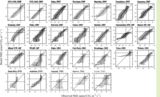
Next, to demonstrate the capability of the proposed model, we compared the observed and predicted values of NEE. Variations in half-hourly or hourly NEE were calculated for all sites during the entire periods for which input meteorological data were

avail-10

able (Fig. 7). The figure plots the class-averaged model-predicted NEE for every 0.5 or 1µmol CO2m

−2

s−1 class against the corresponding observed NEE. Despite the fact that this was a very simple model based on empirical regression methods, it showed good performance for half-hourly or hourly variations in NEE over long pe-riods, especially for forest biomes, and the deviations from the one-to-one line were

15

not large. These results imply that the nonrectangular hyperbola with biome-specific seasonality of physiological parameters can be applied to various biomes to predict diurnal variation in NEE. However, at some of the sites, especially in tundra, the model-predicted NEE was overestimated or underestimated when compared with the observed one, although the magnitude of NEE variability was small (between−4 and

20

2µmol CO₂m−2s−1). It should be noted that the eddy covariance CO₂flux data ana-lyzed include some degree of scatter by random measurement error, which limits the agreement between data and model (Richardson and Hollinger, 2005). Therefore, the discrepancy between the observed and predicted NEE is in part probably due to this uncertainty in measurement.

25

(14)

mid-BGD

5, 4001–4034, 2008

M. Saito et al.

Title Page

Tables Figures

◭ ◮

Back Close

Full Screen / Esc

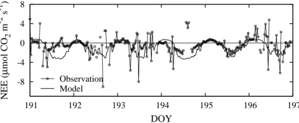
dle of July 2004 (Fig. 8). The discrepancies are obvious during the daytime on DOY 191 and 194. Some of the observed half-hourly NEEs have positive values (indicating CO2release from the ecosystem) during the daytime. The large disagreement at

Atqa-suk resulted in part from this variability in the observed data. However, despite the very small fluctuations in NEE (within±4µmol CO2m

−2

s−1), Fig. 8 shows that the diurnal

5

variation and the magnitude of the predicted NEE were in reasonable agreement with the observations.

The poor agreement between the observed and predicted NEE at some of grassland sites (Fig. 7) is attributable mainly to the disturbance caused by field management at these sites. However, intermediate hardwood and WLEF sites in mixed forests also

10

exhibited large discrepancies in half-hourly NEE variations. The four mixed-forest sites analyzed were closed to each other (see Table 1), so environmental conditions differed little among the sites. As a consequence, it was difficult to determine regression lines characteristic of the relationship between the physiological parameters and environ-mental factors at each of these sites. This is a limitation of the proposed

empirical-15

regression-based model. Further studies of mixed forests using data obtained at diff er-ent sites covering various ranges in temperature, VPD, and precipitation variability are therefore needed to validate the model.

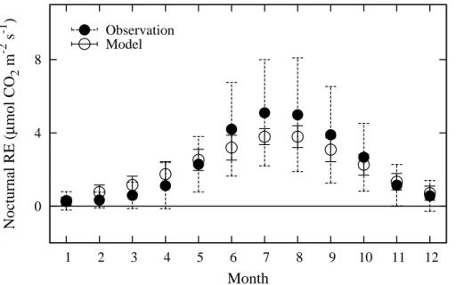
3.3 Nocturnal RE

As mentioned above, the model uses the response of the daytime ecosystem

respi-20

ration to temperature in order to estimate RE variability between both daytime and nighttime over the entire period. The half-hourly or hourly nocturnal RE variability pre-dicted by the model, being mainly indicated by positive NEE values (Figs. 7 and 8), seems to be adequately close to the observed variability. To demonstrate the ability of the model to predict RE variability, as the typical example we show the seasonal course

25

(15)

BGD

5, 4001–4034, 2008

M. Saito et al.

Title Page

Tables Figures

◭ ◮

Back Close

Full Screen / Esc

smaller than those of the observation data. The model slightly overestimates RE in winter and underestimates in summer; the di_fference between the observations and the model is within approximately 1µmol CO2m−

2

s−1.

This difference could be, in part, attributed to the simplifying approach of the model. In the interest of constructing the model as simply as possible, RE variability over a

5

year was introduced with a single equation as a function of temperature, regardless of any differences between growing seasons and non-growing seasons. A recent study by Sampson et al. (2007), however, has demonstrated that there is considerable vari-ability in the temperature dependence of soil respiration in association with seasonal differences in photosynthesis. They suggest that the temperature response of soil

10

respiration increases with increasing photosynthetic rate owing to enhanced substrate supply. However, to avoid complexity and obviate the need to obtain additional infor-mation on the mechanics of the relationship between RE and photosynthesis rate, the model does not account for the influence of these physiological activities on RE. On the other hand, as shown by the large error bars in Fig. 9, it is also clear that the

noctur-15

nal eddy covariance data provide large scatter associated with weak turbulence. This noise is mainly due to flux sampling error, which may, in part, be the cause of the dif-ference between the observed and predicted RE. In view of these problems with both the observation data and the model predictions, we consider that the model estimated diurnal and seasonal variability in RE with moderate accuracy, although it is important

20

to be aware of the abovementioned problems when computing RE variability with the model.

4 Conclusions

We explored a simple approach to predicting diurnal variation in NEE over seven biomes and proposed an empirical model based on the use of a nonrectangular

hyper-25

(16)

BGD

5, 4001–4034, 2008

M. Saito et al.

Title Page

Tables Figures

◭ ◮

Back Close

Full Screen / Esc

exhibited seasonal variations. We showed that this seasonality in parameters could be adequately expressed as a function of environmental variables – air temperature, VPD, annual mean air temperature, and annual precipitation – at the site. The pro-posed model successfully predicted the diurnal variability in NEE for various biomes – especially for forest biomes – over the entire yearly observation period, although

uncer-5

tainties remain in the case of disturbed grassland and savanna biomes. The approach used here would be applicable to other regions. Adjustment of the methodology used in the parameter estimations and subdivision of the biome types would further improve the precision of the model.

Acknowledgements. This study is part of the GOSAT project promoted by the Japan Aerospace 10

Exploration Agency, the National Institute for Environmental Studies, Japan, and the Ministry of the Environment, Japan. We acknowledge Yanhong Tang for useful comments on the manuscript. We also acknowledge NOAA Earth System Research Laboratory and Pennsyl-vania State University for providing the data. Funding for research at Bartlett and Howland AmeriFlux sites was provided by the Northeastern States Research Cooperative, the US. De-15

partment of Energy’s Office of Science (BER) through the Northeastern Regional Center of the National Institute for Climatic Change Research and the Terrestrial Carbon Program un-der Interagency Agreemant No. DE-AI02-00ER63028, with additional support from the USDA Forest Service’s Northern Global Change program and Northern Research Station. G. Katul acknowledges support from the US Department of Energy (DOE) through the O_ffice of Biolog-20

ical and Environmental Research (BER) Terrestrial Carbon Processes (TCP) program (Grants No. 10509-0152, DE-FG02-00ER53015, and DE-FG02-95ER62083).

References

Adams, J. M., Faure, H., Faure-Denard, L., McGlade, J. M., and Woodward, F. I.: Increases in terrestrial carbon storage from the last glacial maximum to the present, Nature, 348, 711– 25

714, 1990. 4011

(17)

BGD

5, 4001–4034, 2008

M. Saito et al.

Title Page

Tables Figures

◭ ◮

Back Close

Full Screen / Esc

R., Verma, S., Vesala, T., Wilson, K., and Wofsy, S.: FLUXNET: a new tool to study the temporal and spatial variability of ecosystem-scale carbon dioxide, water vapor and energy flux densities, B. Am. Meteorol. Soc., 82, 2415–2434, 2001. 4003

Bonan, G. B.: A land surface model (LSM version 1.0) for ecological, hydrological, and at-mospheric studies: Technical description and user’s guide, NCAR Tech. Note NCAR/TN-5

417+STR, 150 pp., 1996. 4003

Bonan, G. B.: The land surface climatology of the NCAR Land Surface Model coupled to the NCAR Community Climate Model, J. Climate, 11, 1307–1326, 1998. 4003

Cao, G., Tang, Y., Mo, W., Wang, Y., Li, Y., and Zhao, X.: Grazing intensity alters soil respiration in an alpine meadow on the Tibetan plateau, Soil Biol. Biochem., 36, 237–243, 2004. 4012 10

Dore, S., Hymus, G. J., Johnson, D. P., Hinkle, C. R., Valentini, R., and Drake, B. G.: Cross validation of open-top chamber and eddy covariance measurements of ecosystem CO₂ ex-change in a Florida scrub-oak ecosystem, Global Change Biol., 9, 84–95, 2003. 4023 Ehleringer, J. and Bj ¨orkman, O.: Quantum yield for CO₂ uptake in C₃ and C₄ plants, Plant

Physiol., 59, 86–90, 1977. 4010 15

Ehleringer, J. and Pearcy, R. W.: Variation in quantum yield for CO₂uptake among C₃ and C₄ plants, Plant Physiol., 73, 555–559, 1983. 4010

Epstein, H. E., Calef, M. P., Walker, M. D., Chapin, F. S., and Starfield, A. M.: Detecting changes in arctic tundra plant communities in response to warming over decadal time scales, Global Change Biol., 10, 1325–1334, 2004. 4023

20

Eugster, W., Rouse, W. R., Pielke, R. A., McFadden, J. P., Baldocchi, D. D., Kittel, T. G. F., Chapin, F. S., Liston, G. E., Vidale, P. L., Vaganov, E., and Chambers, S.: Land-atmosphere energy exchange in Arctic tundra and boreal forest: available data and feedbacks to climate, Global Change Biol., 6, 84–115, 2000. 4023

Falge, E., Baldocchi, D., Olson, R., Anthoni, P., Aubinet, M., Bernhofer, C., Burba, G., Ceule-25

mans, R., Clement, R., Dolman, H., Granier, A., Gross, P., Gr ¨unwald, T., Hollinger, D., Jensen, N. O., Katul, G., Keronen, P., Kowalski, A., Lai, C. T., Law, B. E., Meyers, T., Mon-crie_ff, J., Moors, E., Munger, J. W., Pilegaard, K., Rannik, ¨U., Rebmann, C., Suyker, A., Tenhunen, J., Tu, K., Verma, S., Vesala, T., Wilson, K., and Wofsy, S.: Gap filling strategies for defensible annual sums of net ecosystem exchange, Agr. Forest Meteorol., 107, 43–69, 30

2001. 4008

(18)

BGD

5, 4001–4034, 2008

M. Saito et al.

Title Page

Tables Figures

◭ ◮

Back Close

Full Screen / Esc

Guð_{mundsson, J., Hollinger, D., Kowalski, A. S., Katul, G., Law, B. E., Malhi, Y., Meyers,}

T., Monson, R. K., Munger, J. W., Oechel, W., Paw U, K. T., Pilegaard, K., Rannik, ¨U., Rebmann, C., Suyker, A., Valentini, R., Wilson, K., and Wofsy, S.: Seasonality of ecosystem respiration and gross primary production as derived from FLUXNET measurements, Agr. Forest Meteorol., 113, 53–74, 2002. 4009

5

Farquhar, G. D., von Caemmerer, S., and Berry, J. A.: A biochemical model of photosynthetic CO₂assimilation in leaves of C₃species, Planta, 149, 78–90, 1980. 4003

Fung, I. Y., Tucker, C. J., and Prentice, K. C.: Application of Advanced Very High Resolution Radiometer vegetation index to study atmosphere-biosphere exchange of CO₂, J. Geophys. Res., 92, 2999–3015, 1987. 4002

10

Gholz, H. L. and Clark, K. L.: Energy exchange across a chronosequence of slash pine forests in Florida, Agr. Forest Meteorol., 112, 87–102, 2002. 4023

Gilmanov, T. G., Verma, S. B., Sims, P. L., Meyers, T. P., Bradford, J. A., Burba, G. G., and Suyker, A. E.: Gross primary production and light response parameters of four Southern Plains ecosystems estimated using long-term CO₂-flux tower measurements, Global Bio-15

geochem. Cy., 17, 1071, doi:10.1029/2002GB002023, 2003. 4005, 4007, 4009

Gilmanov, T. G., Tieszen, L. L., Wylie, B. K., Flanagan, L. B., Frank, A. B., Haferkamp, M. R., Meyers, T. P., and Morgan, J. A.: Integration of CO₂ flux and remotely-sensed data for pri-mary production and ecosystem respiration analyses in the Northern Great Plains: potential for quantitative spatial extrapolation, Global Ecol. Biogeogr., 14, 271–292, 2005. 4023 20

Gilmanov, T. G., Soussana, J. F., Aires, L., Ammann, C., Balzarola, M., Barcza, Z., Bernhofer, C., Campbell, C. L., Cernusca, A., Cescatti, A., Clifton-Brown, J., Dirks, B. O. M., Dore, S., Eugster, W., Fuhrer, J., Gimeno, C., Gruenwald, T., Haszpra, L., Hensen, A., Ibrom, A., Jacobs, A. F. G., Jones, M. B., Lanigan, G., Laurila, T., Lohila, A., Manca, G., Marcolla, B., Nagy, Z., Pilegaard, K., Pinter, K., Pio, C., Raschi, A., Rogiers, N., Sanz, M. J., Stefani, P., 25

Sutton, M., Tuba, Z., Valentini, R., and Williams, M. L.: Partitioning European grassland net ecosystem CO₂ exchange into gross primary productivity and ecosystem respiration using light response function analysis, Agric. Ecosyst. Environ., 121, 93–120, 2007. 4008

Goulden, M. L., Munger, J. W., Fan, S. M., Daube, B. C., and Wofsy, S. C.: Measurements of carbon sequestration by long-term eddy covariance: methods and a critical evaluation of 30

accuracy, Global Change Biol., 2, 169–182, 1996. 4009, 4023

(19)

condi-BGD

5, 4001–4034, 2008

M. Saito et al.

Title Page

Tables Figures

◭ ◮

Back Close

Full Screen / Esc

tions and soil moisture on surface energy partitioning revealed by a prolonged drought at a temperate forest site, J. Geophys. Res., 111, D16102, doi:10.1029/2006JD007161, 2006. 4023

Gutschick, V. P.: Joining leaf photosynthesis models and canopy photon-transport models, in: Photon-Vegetation Interaction: Applications in Optical Remote Sensing and Plant Ecology, 5

edited by: Myneni, R. B. and Ross, J., 505–535, Springer-Verlag, 1991. 4005

Hargrove, W. W., Hoffman, F. M., and Law, B. E.: New analysis reveals representativeness of AmeriFlux network, Eos Trans. AGU, 84, 529, 2003. 4004

Hirata, R., Saigusa, N., Yamamoto, S., Ohtani, Y., Ide, R., Asanuma, J., Gamo, M., Hirano, T., Kondo, H., Kosugi, Y., Li, S., Nakai, Y., Takagi, K., Tani, M., and Wang, H.: Spatial distribution 10

of carbon balance in forest ecosystems across East Asia, Agr. Forest Meteorol., 148, 761– 775, 2008. 4005

Hollinger, D. Y., Aber, J., Dail, B., Davidson, E. A., Goltz, S. M., Hughes, H., Leclerc, M., Lee, J. T., Richrdson, A. D., Rodrigues, C., Scott, N. A., Varier, D., and Walsh, J.: Spatial and temporal variability in forest-atmospheric CO₂ exchange, Global Change Biol., 10, 1689– 15

1706, 2004. 4023

Ito, A. and Oikawa, T.: A simulation model of the carbon cycle in land ecosystems (Sim-CYCLE): a description based on dry-matter production theory and plot-scale validation, Ecol. Model., 151, 143–176, 2002. 4006

Jenkins, J. P., Richardson, A. D., Braswell, B. H., Ollinger, S. V., Hollinger, D. Y., and Smith, 20

M. L.: Refining light-use efficiency calculations for a deciduous forest canopy using simulta-neous tower-based carbon flux and radiometric measurements, Agr. Forest Meteorol., 143, 64–79, 2007. 4023

Johnson, I. R. and Thornley, J. H. M.: A model of instantaneous and daily canopy photosynthe-sis, J. Theor. Biol., 107, 531–545, 1984. 4005

25

Katul, G., Leuning, R., and Oren, R.: Relationship between plant hydraulic and biochemical properties derived from a steady-state coupled water and carbon transport model, Plant Cell Environ., 26, 339–350, 2003. 4023

Katul, G. G., Hsieh, C., Bowling, D., Clark, K., Shurpali, N., Turnipseed, A., Albertson, J., Tu, K., Hollinger, D., Evans, B., Offerle, B., Anderson, D., Ellsworth, D., Vogel, C., and Oren, R.: 30

Spatial variability of turbulent fluxes in the roughness sublayer of an even-aged pine forest, Bound.-Lay. Meteorol., 93, 1–28, 1999. 4023

(20)

BGD

5, 4001–4034, 2008

M. Saito et al.

Title Page

Tables Figures

◭ ◮

Back Close

Full Screen / Esc

Groups, Springer-Verlag, 513 pp., 2003. 4011

LeMone, M. A., Grossman, R. L., McMillen, R. T., Liou, K. N., Ou, S. C., McKeen, S., Angevine, W., Ikeda, K., and Chen, F.: Cases-97: Late-morning warming and moistening of the con-vective boundary layer over the Walnut River Watershed, Bound.-Lay. Meteorol., 104, 1–52, 2002. 4023

5

Leuning, R.: Modeling stomatal behavior and photosynthesis ofEucalyptus grandis, Aust. J. Plant Physiol., 17, 159–175, 1990. 4006

Leuning, R., Cleugh, H. A., Zegelin, S. J., and Hughes, D.: Carbon and water fluxes over a temperateEucalyptusforest and a tropical wet/dry savanna in Australia: measurements and comparison with MODIS remote sensing estimates, Agr. Forest Meteorol., 129, 151–173, 10

2005. 4012, 4013

Lieth, H.: Modeling the primary productivity of the world, in: Primary Productivity of the Bio-sphere, edited by: Lieth, H. and Whittaker, R. H., 237–263, Springer-Verlag, 1975. 4007 Lloyd, J. and Taylor, J. A.: On the temperature dependence of soil respiration, Funct. Ecol., 8,

315–323, 1994. 4008 15

Ma, S., Baldocchi, D. D., Xu, L., and Hehn, T.: Inter-annual variability in carbon dioxide ex-change of an oak/grass savanna and open grassland in California, Agr. Forest Meteorol., 147, 157–171, 2007. 4012, 4023

Martens, C. S., Shay, T. J., Mendlovitz, H. P., Matross, D. M., Saleska, S. R., Wofsy, S. C., Woodward, W. S., Menton, M. C., De Moura, J. M. S., Crill, P. M., De Moraes, O. L. L., and 20

Lima, R. L.: Radon fluxes in tropical forest ecosystems of Brazilian Amazonia: night-time CO₂ net ecosystem exchange derived from radon and eddy covariance methods, Global Change Biol., 10, 618–629, 2004. 4023

McMillan, A. M. S., Winston, G. C., and Goulden, M. L.: Age-dependent response of boreal forest to temperature and rainfall variability, Global Change Biol., 14, 1904–1916, 2008. 4023 25

Monteith, J. L.: Solar radiation and productivity in tropical ecosystems, J. Appl. Ecol., 9, 747– 766, 1972. 4003

Nemry, B., Francois, L., G ´erard, J. C., Bondeau, A., Heimann, M., and the participants of the Potsdam NPP Model Intercomparison: Comparing global models of terrestrial net primary productivity (NPP): analysis of the seasonal atmospheric CO₂signal, Global Change Biol., 30

5, 65–76, 1999. 4002

(21)

BGD

5, 4001–4034, 2008

M. Saito et al.

Title Page

Tables Figures

◭ ◮

Back Close

Full Screen / Esc

T., Hadley, J., Heinesch, B., Hollinger, D., Knohl, A., Kutsch, W., Lohila, A., Meyers, T., Moors, E., Moureau, C., Pilegaard, K., Saigusa, N., Verma, S., Vesala, T., and Vogel, C.: Linking flux network measurements to continental scale simulations: ecosystem carbon dioxide ex-change capacity under non-water-stressed conditions, Global Change Biol., 13, 734–760, 2007. 4007, 4010

5

Peat, W. E.: Relationships between photosynthesis and light intensity in the tomato, Ann. Bot. London, 34, 319–328, 1970. 4005

Potter, C. S., Randerson, J. T., Field, C. B., Matson, P. A., Vitousek, P. M., Moonet, H. A., and Klooster, S. A.: Terrestrial ecosystem production: a process model based on global satellite and surface data, Global Biogeochem. Cy., 7, 811–841, 1993. 4003

10

Rabinowitch, E. I.: Photosynthesis and Related Processes, Interscience Publishers, 608 pp., 1951. 4005

Raich, J. W., Rastetter, E. B., Melillo, J. M., Kicklighter, D. W., Grace, A. L., Moore III, B., and V ¨or ¨osmarty, C. J.: Potential net primary productivity in South America: application of a global model, Econ. Appl., 1, 399–429, 1991. 4006

15

Randerson, J. T., Thompson, M. V., Conway, T. J., Fung, I. Y., and Field, C. B.: The contribution of terrestrial sources and sinks to trends in the seasonal cycle of atmospheric carbon dioxide, Global Biogeochem. Cy., 11, 535–560, 1997. 4003

Reichstein, M., Tenhunen, J. D., Roupsard, O., Ourcival, J.-. M., Rambal, S., Miglietta, F., Per-essotti, A., Pecchiari, M., Tirone, G., and Valentini, R.: Severe drought effects on ecosystem 20

CO₂and H₂O fluxes at three Mediterranean evergreen sites: revision of current hypotheses?, Global Change Biol., 8, 999–1017, 2002. 4008

Reichstein, M., Falge, E., Baldocchi, D., Papale, D., Aubinet, M., Berbigier, P., Bernhofer, C., Buchmann, N., Gilmanov, T., Granier, A., Gr ünwald, T., Havr ánkov á, K., Ilvesniemi, H., Janous, D., Knohl, A., Laurila, T., Lohila, A., Loustau, D., Matteucci, G., Meyers, T., Migli-25

etta, F., Ourcival, J. M., Pumpanen, J., Rambal, S., Rotenberg, E., Sanz, M., Tenhunen, J., Seufert, G., Vaccari, F., Vesala, T., Yakir, D., and Valentini, R.: On the separation of net ecosystem exchange into assimilation and ecosystem respiration: review and improved algorithm, Global Change Biol., 11, 1424–1439, 2005. 4008

Richardson, A. D. and Hollinger, D. Y.: Statistical modeling of ecosystem respiration using eddy 30

(22)

BGD

5, 4001–4034, 2008

M. Saito et al.

Title Page

Tables Figures

◭ ◮

Back Close

Full Screen / Esc

Ruimy, A., Dedieu, G., and Saugier, B.: TURC: a diagnostic model of continental gross primary productivity and net primary productivity, Global Biogeochem. Cy., 10, 269–285, 1996. 4003 Sampson, D. A., Janssens, I. A., Curiel Yuste, J., and Ceulemans, R.: Basal rates of soil respiration are correlated with photosynthesis in a mixed temperate forest, Global Change Biol., 13, 2008–2017, 2007. 4008, 4015

5

Schwarz, P. A., Law, B. E., Williams, M., Irvine, J., Kurpius, M., and Moore, D.: Climatic ver-sus biotic constraints on carbon and water fluxes in seasonally drought-affected ponderosa pine ecosystems, Global Biogeochem. Cy., 18, GB4007, doi:10.1029/2004GB002234, 2004. 4023

Scott, R. L., Jenerette, G. D., Potts, D. L., and Huxman, T. E.: The effect of drought on the water 10

and carbon dioxide exchange of a woody-plant-encroached semiarid grassland, Agr. Forest Meteorol., in review, 2008. 4023

Sellers, P. J., Mintz, Y., Sub, Y. C., and Dalcher, A.: A simple biosphere model (SiB) for use within general circulation models, J. Atmos. Sci., 43, 305–331, 1986. 4003

Suyker, A. E. and Verma, S. B.: Year-round observations of the net ecosystem exchange of 15

carbon dioxide in a native tallgrass prairie, Global Change Biol., 7, 279–289, 2001. 4009 Thornley, J. H. M.: Instantaneous Canopy Photosynthesis: Analytical Expressions for Sun and

Shade Leaves Based on Exponential Light Decay Down the Canopy and an Acclimated Non-rectangular Hyperbola for Leaf Photosynthesis, Ann. Bot., 81, 451–458, 2002. 4003 Vickers, D. and Mahrt, L.: The cospectral gap and turbulent flux calculations, J. Atmos. Ocean. 20

Tech., 20, 660–672, 2003. 4009

Wang, C. K., Bond-Lambery, B., and Gower, S. T.: Carbon distribution of a well- and poorly-drained black spruce fire chronosequence, Global Change Biol., 9, 1066–1079, 2003. 4023 Xu, L. and Baldocchi, D. D.: Seasonal variation in carbon dioxide exchange over a

Mediter-ranean annual grassland in California, Agr. Forest Meteorol., 123, 79–96, 2004. 4008, 4023 25

Yi, C. X., Davis, K. J., Berger, B. W., and Bakwin, P. S.: Long-term observations of the dynamics of the continental planetary boundary layer, J. Atmos. Sci., 58, 1288–1299, 2001. 4023 Yuan, W., Liu, S., Zhou, G., Zhou, G., Tieszen, L. L., Baldocchi, D., Bernhofer, C., Gholz, H.,

Goldstein, A. H., Goulden, M. L., Hollinger, D. Y., Hu, Y., Law, B. E., Stoy, P. C., Vesala, T., and Wofsy, S. C.: Deriving a light use efficiency model from eddy covariance flux data for 30

(23)

BGD

5, 4001–4034, 2008

M. Saito et al.

Title Page

Tables Figures

◭ ◮

Back Close

Full Screen / Esc

Table 1.List of AmeriFlux eddy covariance measurement sites analyzed in this study.

Site, country Year Latitude, longitude Reference

Evergreen needle leaf forest (ENF)

UCI-1930 burn site, Canada 2002–2004 55.91◦N, 98.53◦W Wang et al. (2003) UCI-1850 burn site, Canada 2002–2004 55.88◦N, 98.48◦W McMillan et al. (2008) Duke Forest loblolly pine, USA 2002–2004 35.98◦N, 79.09◦W Katul et al. (1999) Howland forest, USA 2002–2004 45.20◦N, 68.74◦W Hollinger et al. (2004) Metolius, USA 2004–2005 44.45◦N, 121.56◦W Schwarz et al. (2004) Slashpine-Donaldson, USA 2002–2004 29.76◦N, 82.16◦W Gholz and Clark (2002)

Evergreen broad leaf forest (EBF)

Santarem-Km67-Primary Forest, Brazil 2002–2004 2.86◦S, 54.96◦W Martens et al. (2004) Florida-Kennedy Space Center, USA 2004–2006 28.61◦N, 80.67◦W Dore et al. (2003)

Deciduous broad leaf forest (DBF)

Duke Forest hardwoods, USA 2003–2005 35.97◦N, 79.10◦W Katul et al. (2003) Harvard Forest EMS Tower, USA 2001–2003 42.54◦N, 72.17◦W Goulden et al. (1996) Missouri Ozark Site, USA 2005–2006 38.74◦N, 92.20◦W Gu et al. (2006) Bartlett Experimental Forest, USA 2004–2005 44.07◦N, 71.29◦W Jenkins et al. (2007)

Mixed forest (MF)

Intermediate hardwood, USA 2003 46.73◦N, 91.23◦W —– Mature red pine, USA 2003–2005 46.74◦N, 91.17◦W —– Mixed young jack pine, USA 2004 46.65◦N, 91.09◦W —–

Park Falls/WLEF, USA 1997, 1999 45.95◦N, 90.27◦W Yi et al. (2001)

Grassland (GRS)

Duke Forest open field, USA 2002–2004 35.97◦N, 79.09◦W Katul et al. (2003)

Fort Peck, USA 2003–2005 48.31◦N, 105.10◦W —–

Brookings, USA 2005–2006 44.35◦N, 96.84◦W Gilmanov et al. (2005)

Vaira Ranch, USA 2002–2004 38.41◦N, 120.95◦W Xu and Baldocchi (2004); Ma et al. (2007) Walnut River Watershed, USA 2002–2004 37.52◦N, 96.86◦W LeMone et al. (2002)

Savanna (SVN)

Santa Rita Mesquite, USA 2004–2006 31.82◦N, 110.87◦W Scott et al. (2008) Audubon Research Ranch, USA 2004–2006 31.59◦N, 110.51◦W —–

Tundra (TND)

Atqasuk, USA 2004–2006 70.47◦N, 157.41◦W —–

(24)

BGD

5, 4001–4034, 2008

M. Saito et al.

Title Page

Tables Figures

◭ ◮

Back Close

Full Screen / Esc

Table 2.List of ecosystem-specific parameter values.

Types Terms Eq. (3) Eq. (4) Eq. (6) Eq. (7) Eq. (8) AMT Tmax Tmin Topt aFV bFV aPM bPM aIni bIni REref E0 Units ◦C ◦C ◦C ◦C – kPa – – (µmol photon µmol CO2 µmol CO2s−1 –

(25)

BGD

5, 4001–4034, 2008

M. Saito et al.

Title Page

Tables Figures

◭ ◮

Back Close

Full Screen / Esc

0 20 40 60 80

0 200 400 600 800 1000

Unstressed maximum P

max

(

µ

mol CO

2

m

-2 s -1 )

NPP (g C m-2 y-1)

UCI-1930 UCI-1850 Duke Howland Metolius Donaldson

Fig. 1.Relationship between annual NPP and unstressed maximum P_maxin evergreen

(26)

BGD

5, 4001–4034, 2008

M. Saito et al.

Title Page

Tables Figures

◭ ◮

Back Close

Full Screen / Esc

0 0.02 0.04

0 10 20 30

Initial slope

(

µ

mol CO

2

(

µ

mol photon)

-1 )

Pmax (µmol CO₂ m-2 s-1)

Duke Fort Peck Brookings Vaira Walnut

Fig. 2. Relationship between bin-averaged P_max and initial slope α in grassland. Sites are

(27)

BGD

5, 4001–4034, 2008

M. Saito et al.

Title Page

Tables Figures

◭ ◮

Back Close

Full Screen / Esc

0 0.005 0.01 0.015

0 10 20 30

RE / NPP (

µ

mol CO

2

s

-1 / (g C y -1 ))

Temperature (oC)

Santa Rita Audubon

Fig. 3. Relationship between bin-averaged temperature and ecosystem respiration scaled by

(28)

BGD

5, 4001–4034, 2008

M. Saito et al.

Title Page Abstract Introduction Conclusions References Tables Figures ◭ ◮ ◭ ◮ Back Close

Full Screen / Esc

Printer-friendly Version Interactive Discussion 0 20 40 60 80

0 200 400 600 800 1000

Unstressed maximum P

max ( µ mol CO 2 m

-2 s -1)

NPP (g C m-2 y-1)

ENF EBF DBF MF GRS SVN TND 0 0.02 0.04

0 10 20 30 40

Initial slope (

µ mol CO 2 ( µ mol photon) -1)

Pmax (µmol CO₂ m-2 s-1)

ENF EBF DBF MF GRS SVN TND 0 0.01 0.02

-10 0 10 20 30

RE/NPP (

µ

mol CO

2

s

-1 / (g C y -1))

Temperature (oC)

0 0.01 0.02

-10 0 10 20 30

RE/NPP (

µ

mol CO

2

s

-1 / (g C y -1))

Temperature (oC)

(a)

(b)

(c)

(29)

BGD

5, 4001–4034, 2008

M. Saito et al.

Title Page

Tables Figures

◭ ◮

Back Close

Full Screen / Esc

Fig. 4.Distributions of three parameters for seven biomes:(a)Same as Fig. 1, but for all biomes

(30)

BGD

5, 4001–4034, 2008

M. Saito et al.

Title Page

Tables Figures

◭ ◮

Back Close

Full Screen / Esc

Interactive Discussion 0

10 20 30 40

Pmax

(

µ

mol CO

2

m

-2 s -1 )

Observation Model

0 10 20 30 40

0 60 120 180 240 300 360

DOY

0 60 120 180 240 300 360

(a) (b)

(c) (d)

Fig. 5. Seasonal course of weekly averaged P_maxat(a)Duke Forest site, ENF;(b)Santarem

(31)

BGD

5, 4001–4034, 2008

M. Saito et al.

Title Page

Tables Figures

◭ ◮

Back Close

Full Screen / Esc

Interactive Discussion 0

0.02 0.04 0.06

Initial slope (

µ

mol CO

2

(

µ

mol photon)

-1 )

Observation Model

0 0.02 0.04 0.06

0 60 120 180 240 300 360

DOY

0 60 120 180 240 300 360

(a) (b)

(c) (d)

(32)

BGD

5, 4001–4034, 2008

M. Saito et al.

Title Page Abstract Introduction Conclusions References Tables Figures ◭ ◮ ◭ ◮ Back Close

Full Screen / Esc

-10 0

-10 0 -10

0 10

-10 0 10 UCI-1930, ENF -30 -20 -10 0 10

-30 -20 -10 0 10

UCI-1930, ENF UCI-1850, ENF

-20 -10 0 10

UCI-1930, ENF UCI-1850, ENF Duke, ENF

-10 0

UCI-1930, ENF UCI-1850, ENF Duke, ENF Howland, ENF

-20 -10 0 10

UCI-1930, ENF UCI-1850, ENF Duke, ENF Howland, ENF Metolius, ENF

-30 -20 -10 0 10

UCI-1930, ENF UCI-1850, ENF Duke, ENF Howland, ENF Metolius, ENF Donaldson, ENF

-20 -10 0 10

UCI-1930, ENF UCI-1850, ENF Duke, ENF Howland, ENF Metolius, ENF Donaldson, ENF Santarem, EBF

-30 -20 -10 0 10

Kennedy, EBF -30 -20 -10 0 10

-30 -20 -10 0 10

Kennedy, EBF Duke, DBF

-20 -10 0 10

Kennedy, EBF Duke, DBF Harvard, DBF

-20 -10 0 10

Kennedy, EBF Duke, DBF Harvard, DBF Ozark, DBF

-30 -20 -10 0 10 20

Kennedy, EBF Duke, DBF Harvard, DBF Ozark, DBF Bartlett, DBF

-20 -10 0 10

Kennedy, EBF Duke, DBF Harvard, DBF Ozark, DBF Bartlett, DBF Intermediate HW, MF

-20 -10 0 10

Model NEE (

µ

mol CO

2

m

-2 s -1 )

Kennedy, EBF Duke, DBF Harvard, DBF Ozark, DBF Bartlett, DBF Intermediate HW, MF Mature RP, MF

-20 -10 0 10

Mixed YJP, MF

-20 -10 0 10

Mixed YJP, MF WLEF, MF

-10 0 10

Mixed YJP, MF WLEF, MF Duke, GRS

-10 0 10

Mixed YJP, MF WLEF, MF Duke, GRS Fort Peck, GRS

-20 -10 0

Mixed YJP, MF WLEF, MF Duke, GRS Fort Peck, GRS Brookings, GRS

-20 -10 0 10

Mixed YJP, MF WLEF, MF Duke, GRS Fort Peck, GRS Brookings, GRS Vaira, GRS

-10 0 10

Mixed YJP, MF WLEF, MF Duke, GRS Fort Peck, GRS Brookings, GRS Vaira, GRS Walnut, GRS

-20 -10 0 10

Santa Rita, SVN

-4 -2 0 2 4

Santa Rita, SVN Audubon, SVN

-4 -2 0 2

Observed NEE (µmol CO₂ m-2 s-1)

Santa Rita, SVN Audubon, SVN Atqasuk, TND

-4 -2 0 2

Santa Rita, SVN Audubon, SVN Atqasuk, TND Barrow, TND

-4 -2 0 2

Santa Rita, SVN Audubon, SVN Atqasuk, TND Barrow, TND Ivotuk, TND

Fig. 7. Class-averaged half-hourly or hourly variations in predicted and observed NEE for all

(33)

BGD

5, 4001–4034, 2008

M. Saito et al.

Title Page

Tables Figures

◭ ◮

Back Close

Full Screen / Esc

-8 -4 0 4 8

191 192 193 194 195 196 197

NEE (

µ

mol CO

2

m

-2 s -1 )

DOY

Observation Model

Fig. 8. Comparison of observed and predicted half-hourly NEE at Atqasuk during the period