Gustavo Mattos Vasques(1), Maurício Rizzato Coelho(1), Ricardo Oliveira Dart(1), Ronaldo Pereira Oliveira(1) and Wenceslau Geraldes Teixeira(1)
(1)Embrapa Solos, Rua Jardim Botânico, no 1.024, Jardim Botânico, CEP 22460-000 Rio de Janeiro, RJ, Brazil. E-mail: [email protected], [email protected], [email protected], [email protected], [email protected]
Abstract – The objective of this work was to compare ordinary kriging with regression kriging to map soil properties at different depths in a tropical dry forest area in Brazil. The 11 soil properties evaluated were: organic carbon content and stock; bulk density; clay, sand, and silt contents; cation exchange capacity; pH; water retention at field capacity and at permanent wilting point; and available water. Samples were taken from 327 sites at 0.0–0.10, 0.10–0.20, and 0.20–0.40-m depths, in a tropical dry forest area of 102 km2. Stepwise linear regression models for particle-size fractions and water retention properties had the best fit. Relief and parent material covariates were selected in 31 of the 33 models (11 properties at three depths) and vegetation covariates in 29 models. Based on external validation, ordinary kriging obtained higher accuracy for 21 out of 33 property x depth combinations, indicating that the inclusion of a linear trend model before kriging does not necessarily improve predictions. Therefore, for similar studies, the geostatistical methods employed should be compared on a case-by-case basis.
Index terms: caatinga, digital soil mapping, gamma radiometric survey, geostatistics, pedometrics.
Mapeamento de carbono, frações granulométricas e água
do solo em Floresta Tropical Seca no Brasil
Resumo – O objetivo deste trabalho foi comparar krigagem ordinária com regressão-krigagem para mapear atributos do solo, em diferentes profundidades, em área de Floresta Tropical Seca no Brasil. Os 11 atributos do solo avaliados foram: conteúdo e estoque de carbono orgânico; densidade do solo; conteúdos de argila, areia e silte; capacidade de troca catiônica; pH; retenção de água na capacidade de campo e no ponto de murcha permanente; e água disponível. As amostras foram retiradas de 327 locais a 0,0–0,10, 0,10–0,20 e 0,20–0,40 m de profundidade, em área de Floresta Tropical Seca de 102 km2. Os modelos de regressão linear “stepwise” tiveram o melhor ajuste para as frações granulométricas e as propriedades de retenção de água. Foram selecionadas covariáveis de relevo e material de origem em 31 dos 33 modelos (11 atributos em três profundidades) e de vegetação em 29 modelos. Com base na validação externa, a krigagem ordinária obteve maior acurácia para 21 das 33 combinações atributo vs. profundidade, o que é indicativo de que a inclusão de um modelo linear de tendência antes da krigagem não necessariamente melhora as predições. Portanto, para estudos semelhantes, os métodos geoestatísticos empregados devem ser comparados caso a caso.
Termos para indexação: caatinga, mapeamento digital de solos, levantamento gamarradiométrico, geoestatística, pedometria.
Introduction
Tropical dry forests correspond to 42% of the world’s tropical and subtropical forests (Murphy & Lugo, 1986), of which about 54% occur in South America (Miles et al., 2006). In Brazil, and possibly other tropical countries, laws concerning tropical dry forests are ill-defined, grouping them with moister or drier forest types. This creates a conundrum, hindering the proper conservation of this important ecosystem that
serves as a habitat for many endemic species, as well as a food and wood source for traditional peoples, but is still little studied. Soil maps can be used to provide information to support government and private sector decisions for promoting the use and conservation of this poorly-known, threatened ecosystem and for guiding future research (Miles et al., 2006).
and external factors, generating complex spatial patterns (Grunwald, 2009). According to Boucneau et al. (1998), soil spatial predictions can be obtained either by: soil property estimation, using mean and range values from a choropleth soil map, for example; or spatial interpolation, using kriging, for instance. While the former assumes uniformity within mapping units and abrupt changes at their boundaries, the latter assumes that all variation is gradual; however, in reality, soil properties may present both gradual and abrupt changes spatially.
Among spatial interpolation methods, kriging constitutes a best linear unbiased estimator and has been extensively used to map soil properties. One of its variants – regression kriging (RK) – has received special attention as a means to incorporate the variation of soil-forming environmental factors (so-called environmental covariates) into the variation of the target soil property (Knotters et al., 1995; Kravchenko & Robertson, 2007; Vasques et al., 2010). Regression kriging integrates remote, field, and laboratory data, and statistical methods in a quantitative estimation framework for soil property or class mapping – digital soil mapping –, with applications ranging from precision agriculture (Grunwald et al., 2015) to global mapping (Hengl et al., 2014).
Ordinary kriging (OK) and RK are commonly used interpolation methods in digital soil mapping, and have been compared in some studies for mapping various soil properties. Knotters et al. (1995) obtained better results with RK using apparent electrical conductivity as a covariate than with OK or cokriging, when mapping the depth to soft layers (peat or unripe clay) in a 97-ha area in the Netherlands. Kravchenko & Robertson (2007), mapping total carbon using topographic and crop yield as covariates, observed little or no improvement with RK in comparison to OK in 12 sites of 0.36 ha in Michigan, in the United States. In the same country, in Florida, RK outperformed OK for total carbon in three out of five depth intervals (Vasques et al., 2010). As reported in previous studies, preference for RK over OK is not granted nor expected, and there is no clear indication of when to use OK, RK, or any other geostatistical method for more accurate results.
The objective of this work was to compare ordinary kriging with regression kriging to map soil properties at different depths in a tropical dry forest area in Brazil.
Materials and Methods
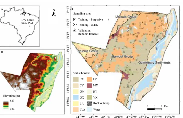
The study was conducted at Parque Estadual da Mata Seca, a dry forest state park, in the north of the state of Minas Gerais, Brazil (43°58'48"W, 14°52'12"S) (Figure 1). The park is located in the ecotone of the Brazilian Atlantic Forest (tropical coastal moist forest), Cerrado (savanna), and Caatinga (xeric shrubland). It was created in 2000 and has been preserved since then. Previously, the land was mainly used for agriculture, cattle ranching, and logging for charcoal production. The study area has 102 km2, encompassing the part of
the park prior to its expansion in 2009. Mean annual temperature and precipitation are around 24°C and 827 mm, respectively.
Vegetation in the study area can be roughly divided into three main types, considering plant species, size, and seasonality: typical dry forest, comprised mostly of deciduous and thorny species that dominate the study area, covering about 69% of the area in the central part; riparian forest, consisting of evergreen species that occur in 25% of the area on richer and moister soils in the eastern part; and “carrasco” forest, characterized by a few thorny and contorted species adapted to poor, sandy, and excessively drained soils, occurring in less than 6% of the area.
Flúvicos (Fluventic Haplustepts), and Neossolos Flúvicos (Ustifluvents, Ustorthents).
Soils were described and sampled at 327 sites, allocated according to three sampling designs, which were carried out in separate field campaigns. In the first design (“survey”), 222 locations were chosen by tacit knowledge for the purpose of soil survey, comprising 44 deep pits (>1 m), 83 shallow pits (<1 m), and 95 boreholes (<1 m). The second design (“cLHS”) consisted of 41 shallow pits allocated by conditioned Latin hypercube sampling (Minasny & McBratney, 2006), using elevation, normalized difference vegetation index, and land use as covariates. The third design (“random transect”) was composed of 64 shallow pits randomly distributed along transects in different directions, cutting across relatively undersampled areas (Figure1).
At all sites, soils were described and classified to the fourth hierarchical level (subgroup) of the Brazilian Soil Classification System (Embrapa, 2013). Sampling was done by horizon in deep pits and by layer in shallow pits and boreholes, at 0.0–0.10, 0.10–0.20, 0.20–0.40, 0.40–0.60, 0.60–0.80, and 0.80–100-m depths. Because soil sampling served different purposes in the experiment, in each field campaign, the shallow pits were sampled differently, with most samples collected at the first three layers to 0.40 m. Undisturbed samples for bulk density (BD) and water retention were obtained using 100-cm3 steel rings. Soil
samples were analyzed in the laboratory according to the methods described by Donagema et al. (2011) for organic carbon (OC), clay, silt, and sand contents (g kg-1); BD (kg dm-3); pH; and water retention
(volumetric percentage) at field capacity (WFC, -0.01
MPa) and at permanent wilting point (PWP, -1.5 MPa). Soil organic carbon stock (OCS, kg m-2) was derived
by multiplying OC, BD, and layer thickness, corrected for the percent of coarse fragments (>2 mm), using the following equation: OCS = 0.01OC × BD × D × (1 - CF/1000), in which OCS is the organic carbon stock (kg m-2), OC is the organic carbon content (g kg-1), BD
is bulk density (kg dm-3), D is layer thickness (cm),
and CF is the coarse fragment (>2 mm) content (g kg -1). Available water (AW, volumetric percentage) was
calculated by subtracting WFC from PWP.
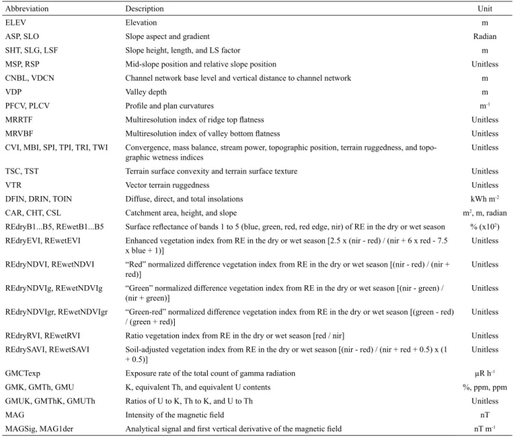
Environmental data layers representing soil-forming factors were compiled in a geographic information system and extracted from the soil sampling sites to be used as model covariates (Table1). A digital elevation model (DEM) was derived from an Ikonos (DigitalGlobe Inc., Westminster, CO, USA) stereo pair from December 2012 with 1-m spatial resolution, and then resampled to 10 m using bilinear interpolation (Figure1 B). Relief covariates were calculated from the resampled DEM. Vegetation covariates were represented by two sets of RapidEye imagery (Planet Labs Inc., San Francisco, CA, USA) with 5-m spatial resolution, one from the
Table 1. Environmental data layers used as model covariates(1).
Abbreviation Description Unit
ELEV Elevation m
ASP, SLO Slope aspect and gradient Radian
SHT, SLG, LSF Slope height, length, and LS factor m
MSP, RSP Mid-slope position and relative slope position Unitless CNBL, VDCN Channel network base level and vertical distance to channel network m
VDP Valley depth m
PFCV, PLCV Profile and plan curvatures m-1
MRRTF Multiresolution index of ridge top flatness Unitless MRVBF Multiresolution index of valley bottom flatness Unitless CVI, MBI, SPI, TPI, TRI, TWI Convergence, mass balance, stream power, topographic position, terrain ruggedness, and topo
-graphic wetness indices
Unitless
TSC, TST Terrain surface convexity and terrain surface texture Unitless
VTR Vector terrain ruggedness Unitless
DFIN, DRIN, TOIN Diffuse, direct, and total insolations kWh m-2
CAR, CHT, CSL Catchment area, height, and slope m2, m, radian
REdryB1...B5, REwetB1...B5 Surface reflectance of bands 1 to 5 (blue, green, red, red edge, nir) of RE in the dry or wet season % (x102)
REdryEVI, REwetEVI Enhanced vegetation index from RE in the dry or wet season [2.5 x (nir - red) / (nir + 6 x red - 7.5
x blue + 1)] Unitless
REdryNDVI, REwetNDVI “Red” normalized difference vegetation index from RE in the dry or wet season [(nir - red) / (nir +
red)] Unitless
REdryNDVIg, REwetNDVIg “Green” normalized difference vegetation index from RE in the dry or wet season [(nir - green) /
(nir + green)] Unitless
REdryNDVIgr, REwetNDVIgr “Green-red” normalized difference vegetation index from RE in the dry or wet season [(green - red)
/ (green + red)] Unitless
REdryRVI, REwetRVI Ratio vegetation index from RE in the dry or wet season [red / nir] Unitless REdrySAVI, REwetSAVI Soil-adjusted vegetation index from RE in the dry or wet season [(nir - red) / (nir + red + 0.5) x (1
+ 0.5)] Unitless
GMCTexp Exposure rate of the total count of gamma radiation µR h-1
GMK, GMTh, GMU K, equivalent Th, and equivalent U contents %, ppm, ppm GMUK, GMThK, GMUTh Ratios of U to K, Th to K, and U to Th Unitless
MAG Intensity of the magnetic field nT
MAGSig, MAG1der Analytical signal and first vertical derivative of the magnetic field nT m-1 (1)nir, near infrared; RE, RapidEye sensor; K, potassium; Th, thorium; U, uranium; kWh, kilowatt-hour; µR, microroentgen; ppm, parts per million; and nT,
dry and the other from the wet season, that is, from August 2012 and May 2013, respectively. The original five bands were radiometrically and atmospherically corrected to surface reflectance, resampled to 10 m by bilinear interpolation, and then used to derive vegetation indices. Parent material covariates included gamma-radiometric and magnetometric layers obtained from an aerial survey (Levantamento..., 2009) with 125-m spatial resolution, which were resampled to 10 m by nearest neighbor resampling. The covariates were processed in the Saga geographic information system (Saga Development Team, University of Hamburg, Hamburg, Germany).
The 11 soil properties evaluated were mapped at the 0.0–0.10, 0.10–0.20, and 0.20–0.40-m depths, respectively. Horizon-based data from the 44 deep pits were recalculated for the three layers by depth-weighted averaging. Model training data was composed of all samples from the survey (222) plus cLHS (41) sets. External model validation data were composed of all 64 random transect samples from a separate field campaign. Descriptive statistics of the soil properties were made, and Pearson’s linear correlations among them were derived.
Two geostatistical methods were compared to map soil properties, namely OK and RK. In RK, the soil properties were first predicted across the study area as a function of the 62 environmental covariates, using stepwise multiple linear regression (SMLR) as a global trend model. Second, the SMLR residuals were interpolated across the area by OK. Then, the SMLR predictions were added to the interpolated residuals to derive the final output maps. Semivariogram models – spherical, exponential, or Gaussian – were chosen visually and were fitted by ordinary least squares and/ or manually.
Stepwise multiple linear regression was implemented using Akaike’s information criterion (AIC) with a p-value of 0.05 for including or excluding variables. All linear regression assumptions were checked. Influential outliers were identified and removed by an outlier test consisting of comparing the Bonferroni corrected p-value from a t-test of the Studentized residuals against a threshold of 0.05. Multicollinearity was minimized by removing variables with variance inflation factors >10.
The goodness-of-fit of the models was assessed by the coefficient of determination (R2), whereas
prediction uncertainty was determined by mean error (ME) for biasedness and by root mean square error (RMSE) for accuracy. The RMSE of the validation was used to select the best geostatistical method for each soil property at each depth. Data analyses were conducted in the R software (R Core Team, 2015).
Results and Discussion
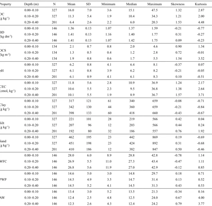
Most soil properties had a close to normal distribution, as indicated by their mean, median, skewness, and kurtosis values (Table2). On average, soils had more sand, followed by clay, then silt. However, particle-size distribution varied according to soil class. Latossolos Amarelos (Haplustox), Latossolos Vermelho-Amarelos (Haplustox, Eutrustox), and Neossolos Flúvicos (Ustifluvents, Usthorthents) had the largest sand content, which decreased with depth. Latossolos Amarelos and Latossolos Vermelho-Amarelos are formed on sand-rich parent material, mainly sandstone, whereas Neossolos Flúvicos are made up of sandy materials deposited on the floodplain of the São Francisco River. Clay content, however, increased with depth, with the largest values found in Vertissolos Háplicos (Haplusterts), Gleissolos Háplicos (Fluvaquents, Endoaqualfs), Cambissolos Háplicos (Haplustepts), and Latossolos Vermelhos (Haplustox, Eutrustox). These soils are formed from clay-richer rocks of the “Bambuí” Group.
Table 2. Descriptive statistics of soil properties(1).
Property Depth (m) N Mean SD Minimum Median Maximum Skewness Kurtosis
OC (g kg-1)
0.00–0.10 327 16.0 7.0 3.6 15.1 47.5 1.32 2.87 0.10–0.20 327 11.3 5.4 1.9 10.4 34.3 1.21 2.00 0.20–0.40 201 6.4 2.6 2.2 6.0 20.3 1.53 4.48
BD (kg dm-3)
0.00–0.10 146 1.36 0.13 1.07 1.37 1.59 -0.21 -0.77 0.10–0.20 146 1.41 0.13 1.16 1.40 1.77 0.31 -0.27 0.20–0.40 146 1.41 0.13 1.07 1.42 1.75 0.09 -0.23
OCS (kg m-2)
0.00–0.10 134 2.1 0.7 0.8 2.0 4.6 0.90 1.34 0.10–0.20 134 1.3 0.5 0.4 1.2 2.8 0.72 -0.01 0.20–0.40 134 1.9 0.8 0.6 1.7 5.5 1.54 3.52
pH
0.00–0.10 327 6.2 0.8 4.1 6.4 8.1 -0.37 0.07 0.10–0.20 327 6.1 0.8 3.9 6.2 8.2 -0.21 -0.05 0.20–0.40 201 6.1 0.9 4.1 6.1 8.3 0.10 -0.51
CEC (cmolc kg-1)
0.00–0.10 327 11.8 5.6 2.8 10.9 36.9 1.24 2.17 0.10–0.20 327 10.6 5.5 2.3 9.5 36.8 1.38 2.64 0.20–0.40 201 10.1 5.5 1.9 8.9 36.7 1.57 3.71
Clay (g kg-1)
0.00–0.10 327 317 121 61 340 659 -0.08 -0.71 0.10–0.20 327 342 130 44 360 659 -0.21 -0.84 0.20–0.40 201 398 133 60 418 660 -0.43 -0.67
Silt (g kg-1)
0.00–0.10 327 221 101 28 219 566 0.42 0.04
0.10–0.20 327 207 96 12 203 566 0.44 0.24
0.20–0.40 201 192 80 32 186 557 0.76 1.92
Sand (g kg-1)
0.00–0.10 327 462 195 23 442 869 0.19 -0.69 0.10–0.20 327 451 198 23 424 892 0.31 -0.68 0.20–0.40 201 410 186 12 382 847 0.50 -0.46
WFC
0.00–0.10 146 28.0 6.0 8.9 28.8 42.8 -0.78 1.14 0.10–0.20 146 26.9 5.5 11.0 27.3 43.4 -0.47 1.11 0.20–0.40 146 26.8 5.6 11.9 27.0 42.9 -0.12 0.85
PWP
0.00–0.10 146 14.6 5.0 3.0 14.8 29.7 0.18 0.71 0.10–0.20 146 14.5 4.9 3.5 14.7 31.4 0.13 0.52 0.20–0.40 146 14.5 5.2 4.1 14.5 31.3 0.43 0.53
AW
0.00–0.10 146 13.4 3.0 5.2 13.5 21.3 -0.34 0.16 0.10–0.20 146 12.4 2.5 4.8 12.5 24.0 0.67 4.00 0.20–0.40 146 12.3 2.6 4.3 12.4 24.2 0.79 3.77
(1)N, number of observations; SD, standard deviation; OC, organic carbon content (g kg-1); BD, bulk density (kg dm-3); OCS, organic carbon stock (kg m-2);
CEC, cation exchange capacity (cmolc kg-1); clay, silt, and sand contents (g kg-1); WFC, water retention at field capacity (volumetric percentage); PWP, water
retention at permanent wilting point (volumetric percentage); and AW, available water (volumetric percentage).
are consistent with those of a previous study in the same region (Oliveira et al., 1998), in which relatively high OC, CEC, and pH were also found in Vertissolos (Vertisols).
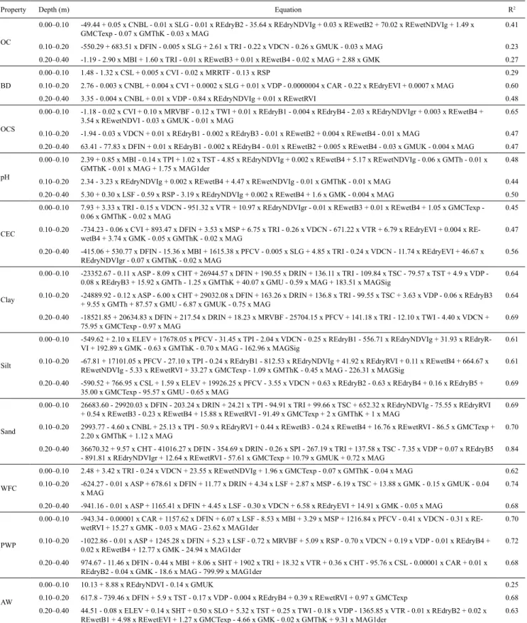
The SMLR models achieved R2 varying from
0.23, for OC at 0–0.10 m, to 0.84, for sand content
depths). Vegetation covariates were selected in 29 models, with general preference for data from the dry (26 models) over the wet (20 models) season. Among the available covariates, the intensity of the magnetic
field (27 models) was by far the most selected variable, followed by diffuse insolation (15 models), ratio of thorium to potassium (13 models), and surface reflectance from RapidEye in the red-edge region (band
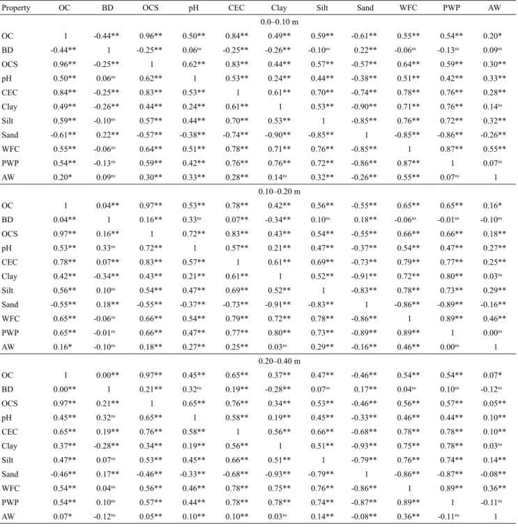
Table 3. Pearson’s linear correlations among soil properties(1).
Property OC BD OCS pH CEC Clay Silt Sand WFC PWP AW 0.0–0.10 m
OC 1 -0.44** 0.96** 0.50** 0.84** 0.49** 0.59** -0.61** 0.55** 0.54** 0.20* BD -0.44** 1 -0.25** 0.06ns -0.25** -0.26** -0.10ns 0.22** -0.06ns -0.13ns 0.09ns
OCS 0.96** -0.25** 1 0.62** 0.83** 0.44** 0.57** -0.57** 0.64** 0.59** 0.30** pH 0.50** 0.06ns 0.62** 1 0.53** 0.24** 0.44** -0.38** 0.51** 0.42** 0.33**
CEC 0.84** -0.25** 0.83** 0.53** 1 0.61** 0.70** -0.74** 0.78** 0.76** 0.28** Clay 0.49** -0.26** 0.44** 0.24** 0.61** 1 0.53** -0.90** 0.71** 0.76** 0.14ns
Silt 0.59** -0.10ns 0.57** 0.44** 0.70** 0.53** 1 -0.85** 0.76** 0.72** 0.32**
Sand -0.61** 0.22** -0.57** -0.38** -0.74** -0.90** -0.85** 1 -0.85** -0.86** -0.26** WFC 0.55** -0.06ns 0.64** 0.51** 0.78** 0.71** 0.76** -0.85** 1 0.87** 0.55**
PWP 0.54** -0.13ns 0.59** 0.42** 0.76** 0.76** 0.72** -0.86** 0.87** 1 0.07ns
AW 0.20* 0.09ns 0.30** 0.33** 0.28** 0.14ns 0.32** -0.26** 0.55** 0.07ns 1
0.10–0.20 m
OC 1 0.04** 0.97** 0.53** 0.78** 0.42** 0.56** -0.55** 0.65** 0.65** 0.16* BD 0.04** 1 0.16** 0.33ns 0.07** -0.34** 0.10ns 0.18** -0.06ns -0.01ns -0.10ns
OCS 0.97** 0.16** 1 0.72** 0.83** 0.43** 0.54** -0.55** 0.66** 0.66** 0.18** pH 0.53** 0.33ns 0.72** 1 0.57** 0.21** 0.47** -0.37** 0.54** 0.47** 0.27**
CEC 0.78** 0.07** 0.83** 0.57** 1 0.61** 0.69** -0.73** 0.79** 0.77** 0.25** Clay 0.42** -0.34** 0.43** 0.21** 0.61** 1 0.52** -0.91** 0.72** 0.80** 0.03ns
Silt 0.56** 0.10ns 0.54** 0.47** 0.69** 0.52** 1 -0.83** 0.78** 0.73** 0.29**
Sand -0.55** 0.18** -0.55** -0.37** -0.73** -0.91** -0.83** 1 -0.86** -0.89** -0.16** WFC 0.65** -0.06ns 0.66** 0.54** 0.79** 0.72** 0.78** -0.86** 1 0.89** 0.46**
PWP 0.65** -0.01ns 0.66** 0.47** 0.77** 0.80** 0.73** -0.89** 0.89** 1 0.00ns
AW 0.16* -0.10ns 0.18** 0.27** 0.25** 0.03ns 0.29** -0.16** 0.46** 0.00ns 1
0.20–0.40 m
OC 1 0.00** 0.97** 0.45** 0.65** 0.37** 0.47** -0.46** 0.54** 0.54** 0.07* BD 0.00** 1 0.21** 0.32ns 0.19** -0.28** 0.07ns 0.17** 0.04ns 0.10ns -0.12ns
OCS 0.97** 0.21** 1 0.65** 0.76** 0.34** 0.53** -0.46** 0.56** 0.57** 0.05** pH 0.45** 0.32ns 0.65** 1 0.58** 0.19** 0.45** -0.33** 0.46** 0.44** 0.10**
CEC 0.65** 0.19** 0.76** 0.58** 1 0.56** 0.66** -0.68** 0.78** 0.78** 0.10** Clay 0.37** -0.28** 0.34** 0.19** 0.56** 1 0.51** -0.93** 0.75** 0.78** 0.03ns
Silt 0.47** 0.07ns 0.53** 0.45** 0.66** 0.51** 1 -0.79** 0.76** 0.74** 0.14**
Sand -0.46** 0.17** -0.46** -0.33** -0.68** -0.93** -0.79** 1 -0.86** -0.87** -0.08** WFC 0.54** 0.04ns 0.56** 0.46** 0.78** 0.75** 0.76** -0.86** 1 0.89** 0.36**
PWP 0.54** 0.10ns 0.57** 0.44** 0.78** 0.78** 0.74** -0.87** 0.89** 1 -0.11ns
AW 0.07* -0.12ns 0.05** 0.10** 0.10** 0.03ns 0.14** -0.08** 0.36** -0.11ns 1
(1)OC, organic carbon content (g kg-1); BD, bulk density (kg dm-3); OCS, organic carbon stock (kg m-2); CEC, cation exchange capacity (cmol
c kg-1); clay,
silt, and sand contents (g kg-1); WFC, water retention at field capacity (volumetric percentage); PWP, water retention at permanent wilting point (volumetric
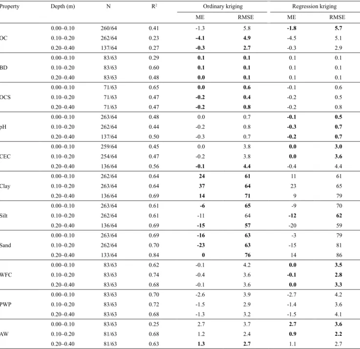
Table 4. Stepwise multiple linear regression model fit and external validation results, with the best geostatistical method in
bold for each property(1).
Property Depth (m) N R2 Ordinary kriging Regression kriging
ME RMSE ME RMSE
OC
0.00–0.10 260/64 0.41 -1.3 5.8 -1.8 5.7
0.10–0.20 262/64 0.23 -4.1 4.9 -4.5 5.1
0.20–0.40 137/64 0.27 -0.3 2.7 -0.3 2.9
BD
0.00–0.10 83/63 0.29 0.1 0.1 0.1 0.1
0.10–0.20 83/63 0.60 0.1 0.1 0.1 0.1
0.20–0.40 83/63 0.48 0.0 0.1 0.1 0.1
OCS
0.00–0.10 71/63 0.65 0.0 0.6 -0.1 0.6
0.10–0.20 71/63 0.47 -0.2 0.4 -0.2 0.5
0.20–0.40 71/63 0.47 -0.2 0.8 -0.2 0.8
pH
0.00–0.10 263/64 0.48 0.0 0.7 -0.1 0.5
0.10–0.20 262/64 0.44 -0.2 0.8 -0.3 0.7
0.20–0.40 137/64 0.50 -0.3 0.7 -0.2 0.7
CEC
0.00–0.10 259/64 0.45 0.0 3.8 0.0 3.0
0.10–0.20 254/64 0.47 -0.2 3.8 0.0 3.6
0.20–0.40 136/64 0.56 -0.1 4.4 -0.4 4.4
Clay
0.00–0.10 262/64 0.64 24 61 11 61
0.10–0.20 263/64 0.64 37 64 23 65
0.20–0.40 136/64 0.69 14 71 9 79
Silt
0.00–0.10 263/64 0.61 -6 65 -9 70
0.10–0.20 262/64 0.61 -11 64 -12 62
0.20–0.40 136/64 0.69 -15 57 -20 59
Sand
0.00–0.10 263/64 0.69 -16 63 -3 79
0.10–0.20 262/64 0.70 -23 63 -15 81
0.20–0.40 133/64 0.84 0 76 14 86
WFC
0.00–0.10 83/63 0.62 -0.1 4.2 0.0 3.5
0.10–0.20 83/63 0.74 -0.4 3.6 -0.1 2.8
0.20–0.40 83/63 0.68 -0.1 3.6 0.0 3.3
PWP
0.00–0.10 83/63 0.70 -2.6 3.9 -2.7 4.2
0.10–0.20 83/63 0.72 -1.5 2.9 -1.4 3.6
0.20–0.40 83/63 0.68 -1.3 3.2 -1.5 4.1
AW
0.00–0.10 83/63 0.25 2.7 3.7 2.7 3.6
0.10–0.20 81/63 0.68 1.2 2.4 0.9 2.2
0.20–0.40 81/63 0.63 1.3 2.7 1.1 2.7
(1)N, number of observations (training/validation); R2, training coefficient of determination; ME, validation mean error; RMSE, validation root mean square
error; OC, organic carbon content (g kg-1); BD, bulk density (kg dm-3); OCS, organic carbon stock (kg m-2); CEC, cation exchange capacity (cmol
c kg-1); clay,
silt, and sand contents (g kg-1); WFC, water retention at field capacity (volumetric percentage); PWP, water retention at permanent wilting point (volumetric
percentage); and AW, available water (volumetric percentage).
4, 690–730 nm) from the wet season (13 models). Red edge is the region where the reflectance of live plants increases from the red (chlorophyll absorption) to the near-infrared region, which has been strongly linked to chlorophyll content, leaf area index, and plant moisture
(Filella & Peñuelas, 1994). The global trend SMLR models of all soil properties are presented in Table5.
makes sense in this region where plant patterns are controlled both by climatic conditions, which regulate evapotranspiration, leaf fall, and phenology (Pezzini et al., 2014), and by soil conditions, which regulate water and nutrient availability (Souza et al., 2007). Oliveira-Filho et al. (1998) identified available light, that is, canopy gaps, as a critical factor controlling the plant species’ abundance distribution in a tropical dry forest in Central Brazil.
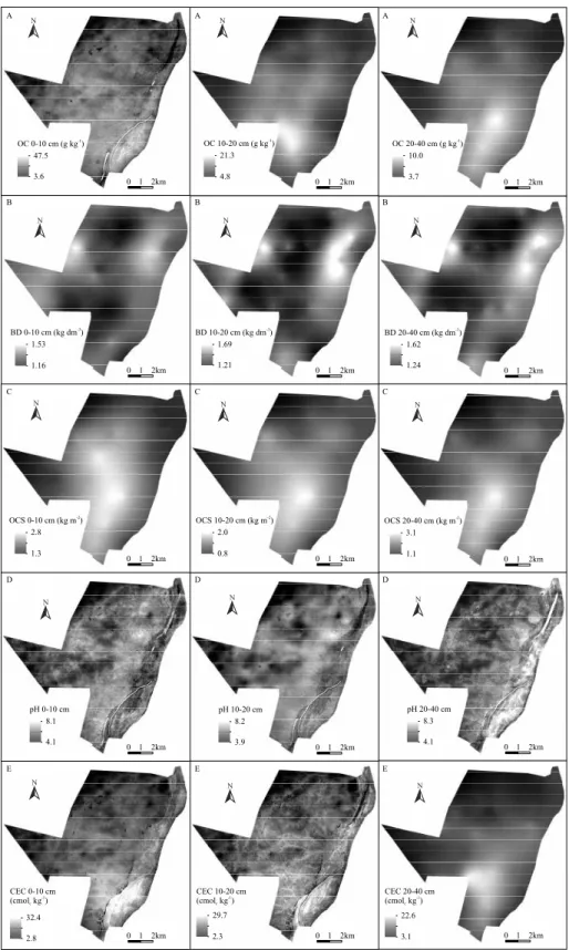
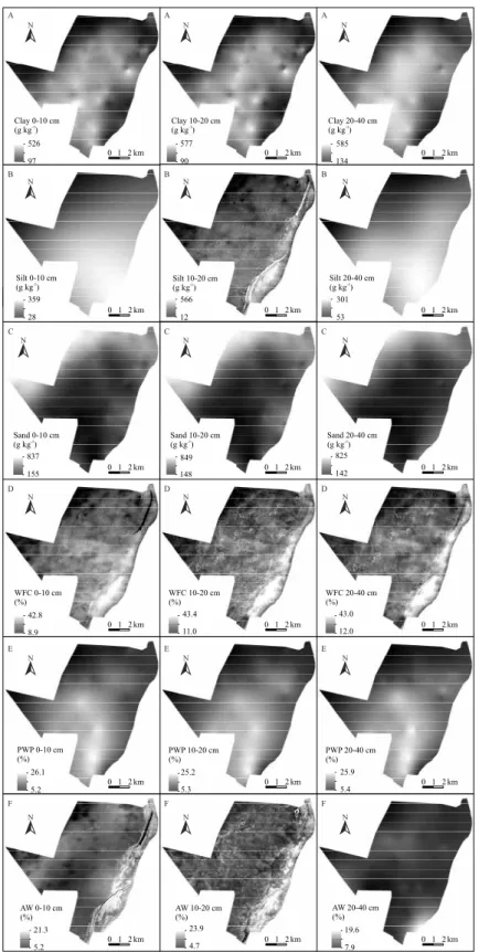
The spatial patterns of the soil properties were related, either positively or negatively (Table 3 and Figures 2 and 3). In the long range, they responded to the variation of geology, which, to some extent, also controls the variation of vegetation. In the short range, they reflected the spatial distribution of soil classes and their properties. The sampling density of about 3.2 samples per square kilometer was enough to derive better OK than RK maps using many (and some costly) environmental covariates for most cases; however, the effect of sampling density on prediction quality was not tested. Since soil properties were correlated, all OK maps look similar. Despite this, the RK maps show differences related to the covariates used in the global trend models, even though they globally resemble the other maps; in addition, the short-range variation of these maps is more detailed according to the variation of the environmental covariates.
The western and northwestern portions of the study area are on sand-rich parent material. These portions have: the sandiest and poorest soils in terms of fertility, that is, low carbon and CEC; low water holding capacity, that is, low WFC, PWP, and AW; and the poorest vegetation of the park, the “carrasco”. The eastern portion constitutes the São Francisco River floodplain, with soils with fluvic characteristics, good water holding capacity, and medium fertility. The central portion corresponds to the area of the “Bambuí” Group, with variable lithology and the presence of calcareous materials, occasionally as rock outcrops. The most common soils in the area are Latossolos Vermelhos and Cambissolos Háplicos, each occupying 31% of the area. Soils with largest carbon stocks, that is, Vertissolos Háplicos and Chernossolos Háplicos, appear in this portion and together occupy less than 3% of the study area.
Total soil OCS at 0.40 m was determined by adding the values obtained at the three depths derived using OK. The study area stores approximately 5.65x10⁵
tons of soil OC in the first 40 cm, of which 34% are found in Cambissolos Háplicos and 30% in Latossolos Vermelhos, due to their large coverage. The “Urucuia” Group, “Bambuí” Group, and “Quaternary sediments” geologic units hold 6, 69, and 24% of the OCS at 0.40 m, respectively, with the largest mean (5.79 kg m-2) in
the “Bambuí” Group.
Considering external validation, OK outperformed RK for 21 out of 33 property x depth combinations, though, for most cases, OK and RK had similar prediction quality (Table 4). The preference for OK over RK did not follow a clear pattern. In fact, in some cases, the best method varied among depths for the same soil property. Nonetheless, this preference still indicates that the local variation of soil properties was, in general, a stronger predictor than environmental covariates. This is regardless of the quality of the SMLR models with RK, which, in some cases, had R2 >0.60
but still performed worse than OK, as observed for clay and sand contents, and PWP. As a rule, the quality of soil predictions depends on soil property, number and distribution of samples, environmental covariates, and soil-landscape correlations, among other factors. It should be noted that neither the number of samples nor the pool of environmental covariates (soil-forming factor groups) was tested in the present study.
Table 5. Stepwise multiple linear regression models for soil properties(1).
Property Depth (m) Equation R2
OC
0.00–0.10 -49.44 + 0.05 x CNBL - 0.01 x SLG - 0.01 x REdryB2 - 35.64 x REdryNDVIg + 0.03 x REwetB2 + 70.02 x REwetNDVIg + 1.49 x
GMCTexp - 0.07 x GMThK - 0.03 x MAG 0.41
0.10–0.20 -550.29 + 683.51 x DFIN - 0.005 x SLG + 2.61 x TRI - 0.22 x VDCN - 0.26 x GMUK - 0.03 x MAG 0.23
0.20–0.40 -1.19 - 2.90 x MBI + 1.60 x TRI - 0.01 x REwetB3 + 0.01 x REwetB4 - 0.02 x MAG + 2.88 x GMK 0.27
BD
0.00–0.10 1.48 - 1.32 x CSL + 0.005 x CVI - 0.02 x MRRTF - 0.13 x RSP 0.29
0.10–0.20 2.76 - 0.003 x CNBL + 0.004 x CVI + 0.0002 x SLG + 0.01 x VDP - 0.0000004 x CAR - 0.22 x REdryEVI + 0.0007 x MAG 0.60
0.20–0.40 3.35 - 0.004 x CNBL + 0.01 x VDP - 0.84 x REdryNDVIg + 0.01 x REwetRVI 0.48
OCS
0.00–0.10 -1.18 - 0.02 x CVI + 0.10 x MRVBF - 0.12 x TWI + 0.01 x REdryB1 - 0.004 x REdryB4 - 2.03 x REdryNDVIgr + 0.003 x REwetB4 +
3.54 x REwetNDVI - 0.03 x GMUK - 0.01 x MAG 0.65
0.10–0.20 -1.94 - 0.03 x VDCN + 0.01 x REdryB1 - 0.002 x REdryB3 - 0.01 x REwetB2 + 0.004 x REwetB4 - 0.01 x MAG 0.47
0.20–0.40 63.41 - 77.83 x DFIN + 0.01 x REdryB1 - 0.002 x REdryB4 - 0.01 x REwetB2 + 0.005 x REwetB4 - 0.03 x GMUK - 0.004 x MAG 0.47
pH
0.00–0.10 2.39 + 0.85 x MBI - 0.14 x TPI + 1.02 x TST - 4.85 x REdryNDVIg + 0.002 x REwetB4 + 5.17 x REwetNDVIg - 0.06 x GMTh - 0.01 x
GMThK - 0.01 x MAG + 1.75 x MAG1der 0.48
0.10–0.20 2.34 - 3.23 x REdryNDVIg + 0.002 x REwetB4 + 4.47 x REwetNDVIg - 0.01 x GMThK - 0.01 x MAG 0.44
0.20–0.40 5.30 + 0.30 x LSF - 0.59 x RSP - 3.19 x REdryNDVIg + 0.002 x REwetB4 + 1.6 x GMK - 0.004 x MAG 0.50
CEC
0.00–0.10 7.93 + 3.33 x TRI - 0.15 x VDCN - 951.32 x VTR + 10.97 x REdryNDVIgr - 0.01 x REwetB3 + 0.01 x REwetB4 + 1.05 x GMCTexp -
0.06 x GMThK - 0.02 x MAG 0.45
0.10–0.20 -734.23 - 0.06 x CVI + 893.47 x DFIN + 3.53 x MSP + 6.75 x TRI - 0.26 x VDCN - 671.22 x VTR + 6.79 x REdryEVI + 0.004 x
RE-wetB4 + 3.74 x GMK - 0.05 x GMThK - 0.02 x MAG 0.47
0.20–0.40 -415.06 + 530.77 x DFIN - 15.36 x MBI + 1615.38 x PFCV - 0.005 x SLG + 4.85 x TRI - 0.24 x VDCN - 11.74 x REdryEVI + 46.67 x
REdryNDVIgr - 0.07 x GMThK - 0.02 x MAG 0.56
Clay
0.00–0.10 -23352.67 - 0.11 x ASP - 8.09 x CHT + 26944.57 x DFIN + 190.55 x DRIN + 136.11 x TRI - 109.84 x TSC - 79.57 x TST + 4.9 x VDP -
0.08 x REdryB3 + 15.92 x GMTh - 1.25 x GMThK + 40.07 x GMU - 0.59 x MAG + 183.51 x MAGSig 0.64
0.10–0.20 -24889.92 - 0.12 x ASP - 6.00 x CHT + 29032.08 x DFIN + 163.26 x DRIN + 136.8 x TRI - 99.55 x TSC + 3.63 x VDP - 0.06 x REdryB3
+ 9.55 x GMTh + 87.57 x GMU - 6.87 x GMUK - 0.75 x MAG 0.64
0.20–0.40 -18521.85 + 20634.83 x DFIN + 217.54 x DRIN + 18.23 x MRVBF - 25704.15 x PFCV + 141.18 x TRI - 12.10 x TWI - 4.40 x VDCN +
75.95 x GMCTexp - 0.97 x MAG 0.69
Silt
0.00–0.10 -549.62 + 2.10 x ELEV + 17678.05 x PFCV - 31.45 x TPI - 2.04 x VDCN - 0.25 x REdryB1 - 556.71 x REdryNDVIg + 31.93 x
REdryR-VI + 192.89 x GMK - 0.63 x GMThK - 0.70 x MAG - 162.96 x MAGSig 0.61
0.10–0.20 -67.81 + 17101.05 x PFCV - 27.10 x TPI - 0.24 x REdryB1 - 812.53 x REdryNDVIg + 41.92 x REdryRVI + 0.11 x REwetB4 + 664.67 x
REwetNDVIg - 5.33 x REwetRVI + 33.27 x GMCTexp - 1.09 x GMThK - 0.45 x MAG - 226.31 x MAGSig 0.61
0.20–0.40 -590.52 + 766.95 x CSL + 1.59 x ELEV + 19926.25 x PFCV - 3.55 x VDCN + 0.63 x REdryB2 - 0.63 x REdryB4 + 0.16 x REdryB5 +
35.00 x GMCTexp - 95.57 x GMU - 0.65 x MAG 0.69
Sand
0.00–0.10 26683.60 - 29920.03 x DFIN - 203.24 x DRIN + 24.21 x TPI - 94.91 x TRI + 99.66 x TSC + 652.32 x REdryNDVIg - 75.55 x REdryRVI
+ 0.54 x REwetB3 - 0.23 x REwetB4 + 15.88 x REwetRVI - 91.49 x GMCTexp + 2 x GMThK + 1 x MAG 0.69
0.10–0.20 2993.77 - 4.60 x CNBL + 25.13 x TPI - 50.9 x REdryRVI + 0.44 x REwetB3 - 0.24 x REwetB4 + 16.76 x REwetRVI - 86.5 x GMCTexp +
2.20 x GMThK + 1.12 x MAG 0.70
0.20–0.40 36670.32 + 9.57 x CHT - 41016.27 x DFIN - 354.69 x DRIN - 0.26 x SPI - 267.19 x TRI + 137.58 x TSC - 7.35 x VDP + 0.07 x REdryB5
- 891.81 x REdryNDVIgr + 12.64 x REwetRVI - 57.61 x GMCTexp + 10.79 x GMUK + 0.72 x MAG 0.84
WFC
0.00–0.10 2.48 + 3.42 x TRI - 0.24 x VDCN + 23.55 x REwetNDVIg + 1.96 x GMCTexp - 0.07 x GMThK - 0.04 x MAG 0.62
0.10–0.20 -624.27 - 0.01 x ASP + 678.61 x DFIN + 11.77 x DRIN + 4.34 x LSF + 2.87 x MSP - 6.19 x TSC + 13.88 x GMK - 0.15 x GMUK - 0.04 x MAG
0.74
0.20–0.40 -941.16 - 0.01 x ASP + 1165.41 x DFIN + 4.45 x LSF - 0.30 x VDCN + 6.58 x REdryEVI + 14.91 x GMK - 0.05 x MAG 0.68
PWP
0.00–0.10 -943.34 - 0.00001 x CAR + 1157.62 x DFIN + 6.07 x LSF - 8.53 x MBI + 3.29 x MSP + 1216.84 x PFCV - 0.41 x VDCN - 0.31 x
RE-wetRVI + 15.27 x GMK - 0.03 x MAG - 23.62 x MAG1der 0.70
0.10–0.20 -1022.86 - 0.01 x ASP + 1245.28 x DFIN + 5.23 x LSF - 0.72 x MRVBF + 5.09 x RSP - 0.70 x VDCN + 0.19 x VDP - 0.01 x REdryB4 +
0.02 x REwetB4 + 12.77 x GMK - 24.94 x MAG1der 0.72
0.20–0.40 974.67 - 11.46 x DFIN - 0.44 x MBI + 8.06 x SHT + 1902 x TRI + 18.32 x VTR + 0.36 x CHT - 95.76 x CSL - 0.00001 x CAR + 0.01 x
REdryB2 - 0.04 x GMK - 18.6 x MAG - 799.99 x MAG1der 0.68
AW
0.00–0.10 10.13 + 8.88 x REdryNDVI - 0.14 x GMUK 0.25
0.10–0.20 617.8 - 739.46 x DFIN + 5.9 x TST - 0.17 x VDP - 0.004 x REdryB4 + 0.39 x REwetRVI + 0.97 x GMCTexp 0.68
0.20–0.40 44.51 - 0.08 x ELEV + 0.14 x SHT + 0.50 x SLO + 5.32 x TST + 0.25 x TWI - 0.18 x VDP - 1365.85 x VTR - 0.01 x REdryB2 + 0.02 x
REwetB1 + 4.98 x REwetEVI + 1.27 x GMCTexp - 4.66 x GMK - 0.02 x GMThK + 9.31 x MAG1der 0.63
(1)R2, training coefficient of determination; OC, organic carbon content (g kg-1); BD, bulk density (kg dm-3); OCS, organic carbon stock (kg m-2); CEC, cation
exchange capacity (cmolc kg-1); clay, silt, and sand contents (g kg-1); WFC, water retention at field capacity (volumetric percentage); PWP, water retention at
Figure 2. Final maps of soil properties based on their best geostatistical methods: A, organic carbon content (OC) at 0.0–0.10-m depth by regression kriging
Figure 3. Final maps of soil properties based on their best geostatistical methods: A, clay content at 0.0–0.10, 0.10–0.20, and 0.20–0.40 m by ordinary kriging
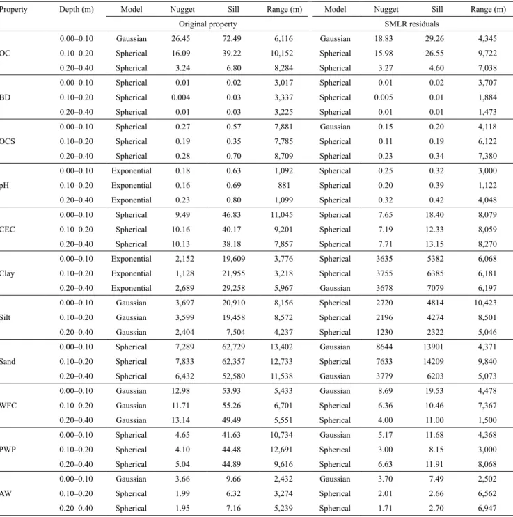
Table 6. Semivariogram parameters for original soil properties and residuals from stepwise multiple linear regression (SMLR)(1).
Property Depth (m) Model Nugget Sill Range (m) Model Nugget Sill Range (m) Original property SMLR residuals
OC
0.00–0.10 Gaussian 26.45 72.49 6,116 Gaussian 18.83 29.26 4,345 0.10–0.20 Spherical 16.09 39.22 10,152 Spherical 15.98 26.55 9,722 0.20–0.40 Spherical 3.24 6.80 8,284 Spherical 3.27 4.60 7,038
BD
0.00–0.10 Spherical 0.01 0.02 3,017 Spherical 0.01 0.02 3,707 0.10–0.20 Spherical 0.004 0.03 3,337 Spherical 0.005 0.01 1,884 0.20–0.40 Spherical 0.01 0.03 3,225 Spherical 0.01 0.01 1,473
OCS
0.00–0.10 Spherical 0.27 0.57 7,881 Gaussian 0.15 0.20 4,118 0.10–0.20 Spherical 0.19 0.35 7,785 Spherical 0.11 0.19 6,122 0.20–0.40 Spherical 0.28 0.70 8,709 Spherical 0.23 0.34 7,380
pH
0.00–0.10 Exponential 0.18 0.63 1,092 Spherical 0.25 0.32 3,000 0.10–0.20 Exponential 0.16 0.69 881 Spherical 0.20 0.39 1,122 0.20–0.40 Exponential 0.23 0.80 1,099 Spherical 0.32 0.42 4,048
CEC
0.00–0.10 Spherical 9.49 46.83 11,045 Spherical 7.65 18.40 8,079 0.10–0.20 Spherical 10.16 40.17 9,201 Spherical 7.19 12.33 8,059 0.20–0.40 Spherical 10.13 38.18 7,857 Spherical 7.71 13.15 8,270
Clay
0.00–0.10 Exponential 2,152 19,609 3,776 Spherical 3635 5382 6,068 0.10–0.20 Exponential 1,128 21,955 3,218 Spherical 3755 6385 6,181 0.20–0.40 Exponential 2,689 29,258 5,967 Gaussian 3678 7079 6,197
Silt
0.00–0.10 Gaussian 3,697 20,910 8,156 Spherical 2720 4814 10,423 0.10–0.20 Gaussian 3,599 19,458 8,572 Spherical 2196 4274 8,501 0.20–0.40 Gaussian 2,404 7,504 4,237 Spherical 1230 2322 5,046
Sand
0.00–0.10 Spherical 7,289 62,729 13,402 Gaussian 8644 13901 4,371 0.10–0.20 Spherical 7,833 62,357 12,733 Spherical 7633 14209 9,840 0.20–0.40 Spherical 6,432 52,580 11,538 Gaussian 3779 6203 5,073
WFC
0.00–0.10 Gaussian 12.98 53.93 5,433 Gaussian 8.69 19.53 4,478 0.10–0.20 Gaussian 11.71 55.26 6,701 Spherical 6.36 10.46 7,367 0.20–0.40 Gaussian 13.14 49.49 5,551 Spherical 4.00 11.00 1,500
PWP
0.00–0.10 Spherical 4.65 41.63 10,734 Gaussian 5.17 11.68 4,368 0.10–0.20 Spherical 4.10 44.48 12,691 Spherical 3.00 8.15 3,000 0.20–0.40 Spherical 5.04 44.89 9,616 Spherical 6.63 11.91 8,068
AW
0.00–0.10 Gaussian 3.66 9.66 2,432 Gaussian 3.70 7.49 2,502 0.10–0.20 Spherical 1.99 6.32 3,274 Spherical 2.01 2.66 6,562 0.20–0.40 Spherical 1.95 7.16 5,239 Spherical 1.71 2.70 6,947
(1)OC, organic carbon content (g kg-1); BD, bulk density (kg dm-3); OCS, organic carbon stock (kg m-2); CEC, cation exchange capacity (cmol
c kg-1); clay,
silt, and sand contents (g kg-1); WFC, water retention at field capacity (volumetric percentage); PWP, water retention at permanent wilting point (volumetric
percentage); and AW, available water (volumetric percentage).
Previous studies have also shown little or no improvement of RK over OK, at plot (Kravchenko & Robertson, 2007), farm/catchment (Zhu & Lin, 2010), or watershed scale (Vasques et al., 2010). Kravchenko
regression model was relatively strong. The same behavior was observed in the present study. In two contrasting landscapes (agricultural versus forested) in the United States, RK was superior to OK only when the spatial structure could not be well captured by point-based observations or when a strong relationship existed between the target soil property and the covariates (Zhu & Lin, 2010). In the same country, in Florida, Vasques et al. (2010) observed that the preference for RK over OK depended on the depth of the measurement and on the regression method used to estimate soil total carbon in a 3,585-km2 watershed.
Studies in tropical dry forest with similar extents or sampling densities were not found to compare with the results obtained in the present study.
Conclusions
1. Soil property patterns are linked to each other, as well as to topographic, geologic, and vegetation patterns in a tropical dry forest area in Brazil.
2. Ordinary kriging is a relatively simple and efficient method to create soil property maps, but it is conditioned to a good sampling design, since, contrary to regression kriging, it only relies on soil samples and not on environmental covariates.
3. There is no straightforward decision on whether to use ordinary kriging or regression kriging for mapping soil properties, because the quality of predictions depends on soil property, number and distribution of samples, environmental covariates, and soil-landscape correlations, among other factors, which indicates that, for similar studies, the employed geostatistical methods should be compared on a case-by-case basis.
Acknowledgements
To Dr. Mário Marcos do Espírito Santo, Dr. Ricardo Luís Louro Berbara, Dr. Maria de Lourdes Mendonça Santos Brefin, to Instituto Estadual de Florestas (IEF) of the state of Minas Gerais, Brazil, to the staff of Parque Estadual da Mata Seca, and to Serviço Geológico do Brasil (CPRM), for support; and to Embrapa (grant No. 03.10.06.013.00.00) and Inter-American Institute for Global Change Research-United States National Science Foundation (grant No. GEO-04523250), for financial support.
References
BOUCNEAU, G.; VAN MEIRVENNE, M.; THAS, O.; HOFMAN, G. Integrating properties of soil map delineations into ordinary kriging. European Journal of Soil Science, v.49, p.213-229, 1998. DOI: 10.1046/j.1365-2389.1998.00157.x.
COELHO, M.R.; DART, R. de O.; VASQUES, G. de M.; TEIXEIRA, W.G.; OLIVEIRA, R.P. de; BREFIN, M. de L.M.;
BERBARA, R.L.L. Levantamento pedológico semi-detalhado
(1:30.000) do Parque Estadual da Mata Seca, município
de Manga-MG. Rio de Janeiro: Embrapa Solos, 2013. 264 p.
(Embrapa Solos. Boletim de pesquisa e desenvolvimento, 217). DONAGEMA, G.K.; CAMPOS, D.V.B. de; CALDERANO, S.B.; TEIXEIRA, W.G.; VIANA, J.H.M. (Org.). Manual de métodos de
análise de solos. 2.ed. rev. Rio de Janeiro: Embrapa Solos, 2011.
230p. (Embrapa Solos. Documentos, 132).
FILELLA, I.; PEÑUELAS, J. The red edge position and shape as indicators of plant chlorophyll content, biomass and hydric status.
International Journal of Remote Sensing, v.15, p.1459-1470,
1994. DOI: 10.1080/01431169408954177.
GRUNWALD, S. Multi-criteria characterization of recent digital soil mapping and modeling approaches. Geoderma, v.152, p.195-207, 2009. DOI: 10.1016/j.geoderma.2009.06.003.
GRUNWALD, S.; VASQUES, G.M.; RIVERO, R.G. Fusion of soil and remote sensing data to model soil properties.
Advances in Agronomy, v.131, p.1-109, 2015. DOI: 10.1016/
bs.agron.2014.12.004.
HENGL, T.; JESUS, J.M. de; MACMILLAN, R.A.; BATJES, N.H.; HEUVELINK, G.B.M.; RIBEIRO, E.; SAMUEL-ROSA, A.; KEMPEN, B.; LEENAARS, J.G.B.; WALSH, M.G.; GONZALEZ, M.R. SoilGrids1km – global soil information based on automated mapping. PLoS ONE, v.9, p.e105992, 2014. DOI: 10.1371/journal.pone.0105992.
KNOTTERS, M.; BRUS, D.J.; OUDE VOSHAAR, J.H. A comparison of kriging, co-kriging and kriging combined with regression for spatial interpolation of horizon depth with censored observations. Geoderma, v.67, p.227-246, 1995. DOI: 10.1016/0016-7061(95)00011-C.
KRAVCHENKO, A.N.; ROBERTSON, G.P. Can topographical and yield data substantially improve total soil carbon mapping by regression kriging? Agronomy Journal, v.99, p.12-17, 2007. DOI: 10.2134/agronj2005.0251.
LEVANTAMENTO aerogeofísico do Estado de Minas Gerais: área 11A (Jaíba – Montes Claros – Bocaiúva). Rio de Janeiro: Serviço Geológico do Brasil, 2009.
MILES, L.; NEWTON, A.C.; DEFRIES, R.S.; RAVILIOUS, C.; MAY, I.; BLYTH, S.; KAPOS, V.; GORDON, J.E. A global overview of the conservation status of tropical dry forests. Journal
of Biogeography, v.33, p.491-505, 2006. DOI:
10.1111/j.1365-2699.2005.01424.x.
MURPHY, P.G.; LUGO, A.E. Ecology of tropical dry forest.
Annual Review of Ecology and Systematics, v.17, p.67-88, 1986.
DOI: 10.1146/annurev.es.17.110186.000435.
OLIVEIRA, C.V.; KER, J.C.; FONTES, L.E.F.; CURI, N.; PINHEIRO, J.C. Química e mineralogia de solos derivados de rochas do Grupo Bambuí no norte de Minas Gerais. Revista
Brasileira de Ciência do Solo, v.22, p.583-593, 1998. DOI:
10.1590/S0100-06831998000400003.
OLIVEIRA-FILHO, A.T.; CURI, N.; VILELA, E.A.; CARVALHO, D.A. Effects of canopy gaps, topography, and soils on the distribution of woody species in a central Brazilian deciduous dry forest. Biotropica, v.30, p.362-375, 1998. DOI: 10.1111/j.1744-7429.1998.tb00071.x.
PEZZINI, F.F.; RANIERI, B.D.; BRANDÃO, D.O.; FERNANDES, G.W.; QUESADA, M.; ESPÍRITO-SANTO, M.M.; JACOBI, C.M. Changes in tree phenology along natural regeneration in a seasonally dry tropical forest. Plant Biosystems, v.148, p.965-974, 2014. DOI: 10.1080/11263504.2013.877530.
R CORE TEAM. R: a language and environment for statistical computing. Vienna: R Foundation for Statistical Computing, 2015.
SOIL SURVEY STAFF. Keys to soil taxonomy. 12nd ed.
Washington: United States Department of Agriculture, 2014. SOUZA, J.P. de; ARAÚJO, G.M.; HARIDASAN, M. Influence of soil fertility on the distribution of tree species in a deciduous forest in the Triângulo Mineiro region of Brazil. Plant Ecology, v.191, p.253-263, 2007. DOI: 10.1007/s11258-006-9240-2.
VASQUES, G.M.; GRUNWALD, S.; COMERFORD, N.B.; SICKMAN, J.O. Regional modelling of soil carbon at multiple depths within a subtropical watershed. Geoderma, v.156, p.326-336, 2010. DOI: 10.1016/j.geoderma.2010.03.002.
ZHU, Q.; LIN, H.S. Comparing ordinary kriging and regression kriging for soil properties in contrasting landscapes. Pedosphere, v.20, p.594-606, 2010. DOI: 10.1016/S1002-0160(10)60049-5.