Optimized exploitation of aquifers: application
to the Querença-Silves aquifer system
J. Ferreira
1, M. C. Cunha
1, J. Vieira
1& J. P. Monteiro
21Department of Civil Engineering, Coimbra University, Portugal 2University of Algarve, Portugal
Abstract
A great deal of optimization models have been developed to support aquifer planning and management with the goal of arriving at the best decisions in relation to the number and siting of infrastructures to be built and how to operate them. A mixed-integer multi-objective linear model has been taken from the literature to define the best decision for the development of the aquifer of Querença-Silves (Portugal). It identifies efficient solutions for the location and design of pumping stations and their catchment area to supply a given number of demand centers, without disregarding the effect of groundwater management on the piezometric surface of aquifers and the many facets of groundwater management. The multi-objective model includes two objectives: (1) the minimization of aggregate water elevation height, and (2) the minimization of aggregate water transport length, weighted by the flows conveyed from the facilities to the centers. The effect of groundwater extraction on the piezometric surface of the aquifer is modelled with a response matrix method, with the establishment of maximum drawdown to prevent over-exploitation.
Keywords: aquifer systems, multiobjective models, mixed-integer models.
1 Introduction
The growing consumption of groundwater around the world has compelled the utmost care in its use so as to avoid problems of over-exploitation and contamination of reserves. Planning the best technical solutions may require the use of decision models that offer a systematic integrated approach to problems. This paper sets out a multi-objective model from the literature conceived to find efficient solutions for the location and design pumping stations and their catchment area to supply a given number of demand centers. The next section
presents the mathematical formulation of the optimization model in question, proposed by Cunha and Antunes [1]. The results of applying this model to a case based on a real situation are also presented. The study assessed the optimal location for a series of groundwater wells in the Querença-Silves aquifer (the most important in Algarve) that would satisfy the demand of a number of centers/localities.
2 Optimization
model
The optimization model proposed by Cunha and Antunes [1] is a mixed-integer multi-objective linear model to identify efficient solutions for locating and designing pumping stations and their catchment areas. The pumping stations correspond to the groundwater wells needed to ensure meeting demand of a certain number of centres/localities. The model includes two objectives: (1) the sum of water-pumping heights which represent a proxy of capital and operating costs for flow extraction, and (2) the sum of the distances considered between the pumping sites and demand centres, weighted by flows conveyed from the facilities to the centers which are a proxy of the transport costs.
J centres/localities are considered and the aquifer is divided into K units called cells. These cells are used to monitor the piezometric surface of the aquifer and to locate the groundwater wells. The purpose of minimizing the total pumping heights H requires two terms. The differences Z between the elevation of the demand centres and the initial piezometric surface of the aquifer in each pumping station are added to the drawdowns R caused by the pumping:
(1) The total drawdown is given by:
(2) : drawdown in cell k.
Drawdowns Rk are calculated with the response matrix method (Maddock
[4]). The use of the response matrix method to calculate drawdowns in the aquifer involves the prior determination of the influence coefficients which represent the drawdown in cell k as a result of the extraction of a unit volume from a well in cell k’:
(3) : flow pumped in cell/catchment k’
The pumped flows are written as the sum of the inputs of each well k’ for the various consumption centres j:
(4) : demand of centre j
: fraction of demand of centre j supplied by site k’
The sum of the differences Z between the elevations of the demand centres and those corresponding to the initial piezometric surface of the aquifer at each pumping site is given by:
(5)
: difference between level of demand centre j and the ground level of site k
: difference between the ground level and the initial piezometric level of the aquifer at site k
: is 1 if centre j is supplied by site k and is 0 otherwise
The reason for using instead of just is related the fact that pumping may not be required when the water is transported by gravity.
The objective of minimizing the sum L of the transport distances considered between pumping sites and demand centres weighted by the flows conveyed from the facilities to the centers may be put in mathematical terms as follows:
(6) : distance between centre j to site k.
Of the model’s other constraints attention is drawn first to the one that ensures the demands of each centre are fully met (expression (7)), and the one that defines the maximum number of wells that can be sunk in the aquifer (expression (8)).
(7)
(8) : is 1 if there is a well in k and 0 otherwise
Other important restrictions are those that define the minimum and maximum flow pumped at each site (expression (9)), the maximum drawdowns for each site (expression (10)) and the minimum flow which would justify sinking a well in the aquifer (expression (11)):
(9) (10)
(11) : minimum flow required to justify a well
: maximum flow at well k : maximum drawdown at well k
: sufficient flow to justify investing in pipes
The list of constraints is completed with two more groups of constraints. The first (expression 12) ensures that the elevation differences between pumping sites and consumption centres will only count when this centre is supplied by this site. The second set of constraints (13) ensures that a consumption centre cannot be supplied by a non-existent well.
(12) (13) As the model proposed by Cunha and Antunes [1] is a mixed-integer multi-objective optimization model it can be resolved with commercially available software like XPRESS-MP [2].
3 Case study: Querença-Silves aquifer
The multi-objective model described above was applied to the Querença-Silves aquifer. This is a karst aquifer system on the southern rim of Portugal’s Algarve region and is the biggest and most important system in that region. The aquifer has some confined zones and others that are freatic. Further details of the aquifer system can be found in SNIRH [6].
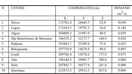
The problem included 10 demand centres and 100 possible well sites. It was assumed that one site could serve several centres and several sites could serve one centre. The maximum flows to be pumped, initial piezometric level in each possible well site and the influence coefficients are based on information provided in Monteiro et al. [5]. The table below gives the coordinates of the centres and consumption considered (Table 1).
Table 1: Demand centre details.
N CENTRE COORDINATES (m) DEMAND (m3/s)
X Y Z
1 Silves 172762.8 24845.3 52.0 0.050 2 Lagoa 171655.5 18792.3 34.0 0.144 3 Algoz 184809.2 21987.0 40.0 0.029 4 São Bartolomeu de Messines 186335.2 32273.7 140.0 0.028 5 Paderne 193881.1 23399.8 75.0 0.025 6 Boliqueime 197729.0 18678.8 90.0 0.007 7 Loulé 209766.4 19276.6 175.0 0.075 8 Alte 196144.5 29983.7 180.0 0.004 9 Salir 207865.7 30577.6 241.0 0.006 10 Querença 212872.5 25912.5 263.0 0.004
The model was tested for a maximum of 5, 15 and 25 wells installations for comparison purposes.
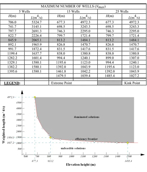
The range of values for each objective was determined in a first step. For this each was individually minimized. Pareto solutions are generated by applying the “ε constraint method”. As such, the model is solved by considering only one of the objectives and including the other objectives as constraints. Successively minimizing one objective, with the value of the other objective fixed with a value within the range obtained in the first step, thus operating as a constraint. The objective chosen to block the value was the sum of the pumping heights (H), and so the objective to be minimized became the one related to transport (L). The solutions obtained allowed the points of the efficient boundary to be found, thereby enabling its shape to be calculated and the “kink point” to be viewed. This point defines a solution that contemplates the two objectives considered in a balanced manner, which is a more realistic solution than those that define the ends. Table 2 presents the solutions belonging to the efficiency frontier for
Table 2: Solutions belonging to the efficiency frontier for Nmax=5, 15 and 25. MAXIMUM NUMBER OF WELLS (Nmax)
5 Wells 15 Wells 25 Wells H(m) L(m4/s) H(m) L(m4/s) H(m) L(m4/s) 706.0 5324.7 677.3 4972.3 677.3 4972.3 741.7 3145.1 698.5 3243.3 698.5 3243.3 797.7 2691.3 746.3 2295.0 746.3 2295.0 822.7 2226.4 799.7 1721.4 799.7 1721.4 845.9 2065.1 813.2 1484.1 813.2 1484.1 892.1 1965.9 826.8 1470.7 826.8 1470.7 991.7 1872.4 831.5 1417.6 831.5 1417.6 1199.4 1637.7 838.0 1380.8 838.0 1380.8 1282.2 1601.4 994.4 1240.1 899.0 1307.0 1329.1 1580.1 1195.6 1123.0 994.4 1240.1 1382.2 1580.1 1392.0 1043.9 1195.6 1123.0 1395.6 1580.1 1461.8 1042.2 1392.0 1043.9 1479.5 1039.4 1485.4 1027.2
LEGEND: Extreme Point Kink Point
Figure 1: Efficient boundary for a limit of 25 wells.
Nmax=5, 15 and 25. Figure 1 displays the Pareto solutions for the case of the
installation of wells being limited by 25.
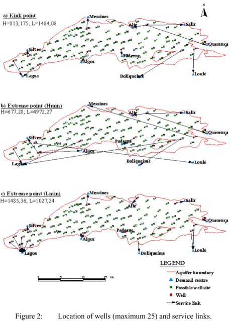
Figure 1 also shows the set of dominated solutions. “kink point” (point where an abrupt change in the outline of the efficient frontier can be seen) and ends. Figure 2 shows the format of the boundary on a map of the aquifer and relative location of the possible well sites. In addition, the service links and location of wells defined by resolving the problem for the extreme situation can be seen (with an objective minimized without considering the other objective as a constraint, end point) and for the “kink point” shown in the previous figure, for a limit of 25 wells.
Figure 2: Location of wells (maximum 25) and service links.
Figure 2 shows that even though the maximum number of wells considered was 25, the optimum solution could be achieved with fewer. In other words, after a certain number of wells the objective function cannot obtain lower values. The same figure also shows that when the intention is to only to minimize pumping heights fewer installations (Figure 2b) corresponding to the extreme point Hmin)
are needed than for the other situations. However, it has service links that cross the whole aquifer, becoming a very costly choice from the point of view of the expense of pipes (laying and maintaining them, and other costs related to transporting the water).
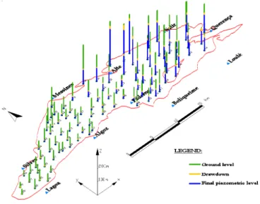
Figure 3: Piezometric map for maximum of 25 wells for the “kink point”. But if the aim is to minimize the transportation distance considered the effect of the demand for the wells to be close to the demand centres is noticed in the high number of them that are required to reduce the value of the objective function (Figure 2c)) corresponding to the extreme point Lmin). In these
circumstances the limitation on the number of wells is felt. This solution could be very high from the economic point of view because of the installation, maintenance and operating costs of the equipment, but it could have the advantage of bringing a certain reliability to the system of wells. Taking the failure of some pumping stations into account, the others would offset this problem to some extent.
When the “kink point” solution is examined (Figure 2a)) this is found to incorporate some of the positive aspects of the two previous solutions, viz. a reasonable amount of equipment and an acceptable total transport distance. It is easy to conclude that the “kink point” solution is the most balanced one and is the most likely to be implemented. In this case an efficient number of wells to sink is 9.
Figure 3 shows the drawdown caused by exploitation the same as at the kink point, for the result obtained for a maximum of 25 wells.
A more detailed analysis of this problem can be found in Ferreira [3].
4 Conclusions
Applying the mixed linear multi-objective model described in Cunha and Antunes [1] to a study based on a real situation leads to the conclusion that this would be a useful tool. It is easy to resolve and helps to determine which wells should be sunk in an aquifer since it provides results consistent with the
objectives proposed: minimizing proxies of pumping and the transport distance costs.
References
[1] Cunha, M.C. & Antunes, A.P., On the efficient location of pumping facilities in an aquifer system. International Transactions in Operational
Research, 4(3), pp. 20-25, 1997.
[2] Dash Optimization, Xpress-MP Getting Started, Blisworth, 2007.
[3] Ferreira, J., Exploração Optimizada de Sistemas Aquíferos, Msc Thesis, Departamento de Engenharia Civil da Universidade de Coimbra, Coimbra, 2008.
[4] Maddock (III), T., Algebraic technological function from a simulation model. Water Resour. Res., 8(1), pp. 129-134, 1972.
[5] Monteiro, J., Vieira, J., Nunes, L. & Fakir, Y., Inverse Calibration of a Regional Flow Model for the Querença-Silves Aquifer System (Algarve-Portugal)”. 1st International Conference on Integrated Water Resources Management and Challenges of the Sustainable Development, International
Association of Hydrogeologists, Marrakech, doc. elect. CD-ROM, 6p, 2006. [6] Sistema Nacional de Informação de Recursos Hídricos (SNIRH), Online,