Monitoring of urban transportation networks using wireless sensor networks

(1)

UNIVERSIDADE DO ALGARVE

Monitoring of Urban Transportation Networks Using

Wireless Sensor Networks

Nuno Miguel G. M. Carvalho

Master Thesis in Computer Science Engineering

Work done under the supervision of: Prof. No´elia Correia

(2)

Statement of Originality

Monitoring of Urban Transportation Networks Using Wireless Sensor Networks Statement of authorship: The work presented in this thesis is, to the best of my knowl-edge and belief, original, except as acknowlknowl-edged in the text. The material has not been submitted, either in whole or in part, for a degree at this or any other university.

Candidate:

(Nuno Miguel G. M. Carvalho)

Copyright c Nuno Miguel G. M. Carvalho. A Universidade do Algarve tem o direito, perpétuo e sem limites geográficos, de arquivar e publicitar este trabalho através de exem-plares impressos reproduzidos em papel ou de forma digital, ou por qualquer outro meio conhecido ou que venha a ser inventado, de o divulgar através de repositórios cient´ıficos e de admitir a sua cópia e distribuição com objetivos educacionais ou de investigação, não comerciais, desde que seja dado crédito ao autor e editor.

(3)

NE T W O R K I N G

Work done at Research Center of Electronics Optoelectronics and Telecommunications (CEOT)

(4)

Abstract

With today’s technologies, constant growth of people in major cities and the permanent concern with our natural resources, such as energy, it is inevitable that we look for ways to improve our urban transportation networks. One way of improving transportation net-works is to make an efficient vehicle routing. In this thesis vehicle routing with backup provisioning, using wireless sensor technologies, is proposed. We start by collecting the entry and exit of people inside urban transportations, which will give us a view of fleet load over time, using wireless sensor technologies. For this purpose a monitoring soft-ware was developed. Such data gathering and monitoring tool will allow data analysis in real time and, according to information extracted, to propose solutions for service im-provements. In this thesis the possibility of using such data to plan vehicle routes with backup provisioning is discussed. That is, a variant of the open vehicle routing prob-lem is proposed, called vehicle routing with backup provisioning, where the possibility of reacting to overloading/overcrowding of vehicles in certain stops is considered. After mathematically formalizing the problem a heuristic algorithm to plan routes is proposed. Results show that vehicle routing with backup provisioning can be a way of providing sustainable urban mobility with efficient use of resources, while increasing quality of ser-vice perceived by users. We expect this tool to be useful for the improvement of Urban Transportation Networks.

Keywords: wireless sensor networks, smart cities, urban traffic system, open vehicle rout-ing problem, monitorrout-ing, trackrout-ing

(5)

Resumo

Com os atuais avanços tecnológicos, o aumento das populações nas grandes cidades e com a constante preocupação com os nossos recursos naturais, como a energia, é essencial sermos mais eficientes e melhorarmos as nossas cidades. Com sensores cada vez mais pequenos, baratos e eficientes, procuramos formas de transformar as nossas cidades em cidades inteligentes.

Este trabalho tem como objetivo melhorar a nossa rede de transportes urbanos. O transporte eficiente de pessoas e bens tem sido estudado nos últimos 50 anos. Milhares de trabalhos foram escritos com várias variantes deste problema de optimização. Mais recentemente foi introduzida uma variante do vehicle routing problem chamada de open vehicle routing problem, que não obriga os ve´ıculos a regressar à origem após concluida a sua última distribuição ou tarefa. O nosso problema, que pelo que sabemos não foi discu-tido na literatura dispon´ıvel, é uma variante do open vehicle routing problem aplicado ao transporte de pessoas, mas com uma carater´ıstica extra que é a possibilidade de fornecer backup a estações cr´ıticas. Ou seja, constru´ımos as rotas de forma a fornecerem backup às estações cr´ıticas caso seja necessário. Este backup é efetuado dentro de um intervalo de tempo definido.

Começamos por recolher as entradas e sa´ıdas de pessoas nos transportes urbanos, o que nos dá uma visão geral da lotação dos ve´ıculos ao longo do tempo, tendo estes da-dos sido recolhida-dos com recurso a sensores sem fios. As redes de sensores sem fios têm sido usadas para monitorização e rastreamento em diversas áreas como: saúde, fornec-imento de energia, monitorização de tráfego, rastreamento de animais e pessoas. Nesta tese vamos usar a monitorização e o rastreamento. Para rastreamento vamos recorrer a nós sensores com passive infrared, e para monitorização vamos desenvolver uma plataforma de visualização dos dados.

O software de monitorização foi desenvolvido com recurso a uma framework Model-View-Controllerde PHP e um software de informação geográfica.

Para a recolha de dados utilizamos sensores da Coalsenses, mais concretamente, o Security Module e o Gateway Module. O primeiro foi usado para recolher os dados e o segundo para encaminhar os mesmos para a nossa plataforma. Ambos os sensores foram configurados com IPv6, mais concretamente com a stack protocolar 6LoWPAN, para dispositivos com energia limitada. O Security Module é composto, entre outros, por um passive infrared. Foi necessário reduzir a área de ação do passive infrared para 20◦

(6)

-30◦graus, em vez dos 110◦ que é o valor padrão para este tipo de sensores. Esta redução é necessária porque precisamos de uma faixa bem definida para a captura de eventos. Os sensores equipados com passive infrared, Security Module, foram configurados de forma a enviarem dados com o seu identificador e com o evento, que neste caso é a passagem de uma pessoa, e após validação estes dados são enviados para o Gateway Module que reencaminha para a nossa plataforma de monitorização. Optámos por colocar dois passive infraredpor porta para podermos detetar a direção na entrada ou sa´ıda.

Com o software de monitorização, e com os dados por ele recolhidos, temos a possi-bilidade de analisar os dados em tempo real, permitindo-nos assim propor soluções para melhorar o serviço prestado. Nesta tese é discutida a possibilidade de analisar estes da-dos para planear rotas com o fornecimento de backup. É proposta uma variante do open vehicle routing problem chamada vehicle routing with backup provisioning, onde é con-siderada a possibilidade de reagir a eventos de sobrelotação dos ve´ıculos em algumas paragens consideradas cr´ıticas. Definimos o nosso problema e posteriormente fizemos a formalização matemática do mesmo. Propusemos ainda uma heur´ıstica para planear ro-tas, na qual definimos dois passos, criação das rotas e inclusão de backup. A inclusão de backup extende, se necessário, as rotas constru´ıdas para permitir o fornecimento de backup a uma estação cr´ıtica dentro de um determinado intervalo de tempo. Vários con-juntos de estações cr´ıticas e intervalos de tempo foram testados e analizados.

Depois de alguns testes para avaliar o desempenho da heurıistica, decidimos, então im-plementar procedimentos pós-optimais para melhorar a performance da nossa heur´ıstica e analisar os resultados utilizando dados conhecidos de vehicle routing problems. Uti-lizámos dados com 52 nós, onde definimos que as estações obrigatórias seriam o nó inicial e o nó mais distante (chamado mandatory, que depois de executada a heur´ıstica poderá ser o nó destino ou não; i.e., poderá haver extensão para além deste mandatory para que seja fornecido backup). Como nós cr´ıticos definimos os nós com mais procura ou de-mand. Os resultados mostram que o vehicle routing with backup provisioning possibilita uma mobilidade urbana sustentável, com uso eficiente de recursos e que os procedimen-tos pós-optimais melhoram significativamente a qualidade das soluções iniciais obtidas pela heur´ıstica. Os resultados mostram que o vehicle routing with backup provisioning pode ser uma solução muito flex´ıvel e de baixo custo para o melhoramento da rede de transportes e ao mesmo tempo melhorar a qualidade da experiência para os utilizadores. Esperamos que esta ferramenta seja útil para melhorar as nossas atuais redes de trans-portes urbanos.

Termos chave: redes de sensores sen fios, smart cities, sistema de tráfego urbano, open vehicle routing problem, monitorização, tracking

(7)

Acknowledgements

This work is dedicated to all those around me, family and friends for all support given, especially:

To my wife and son, who not only supported me but also believed and encouraged not only to finish this work but especially to be a better person. Thank you for all the love, understanding and support given.

My parents and brother who always believed in me.

To Prof. No´elia Correia and Prof. Gabriela Sch¨utz for their help and support in the design and analysis of this work.

To the Research Center of Electronics Optoelectronics and Telecommunications (CEOT) a special thanks in providing not only the sensors but for all the infrastructure and material provided during this thesis.

A special thanks to all that directly or indirectly contributed for this work, professors, friends, ...

(8)

List of Figures

1.1 Vehicle to roadside access point example. . . 3

1.2 Illustration of vehicle routing problem with reactive response to overload. 4 3.1 MVC pattern diagram. . . 10

3.2 Monitoring tool - Home page. . . 10

3.3 Monitoring tool - Adding stations. . . 11

3.4 Monitoring tool - Adding routes. . . 11

3.5 Sensor application in a bus. . . 14

3.6 Architecture and data communication schema. . . 14

3.7 FSM diagram for each sensor node of dual implementation. . . 15

5.1 Intra-route relocation. . . 27

5.2 Intra-route exchange. . . 27

5.3 Inter-route relocation. . . 28

5.4 Inter-route cross-exchange. . . 28

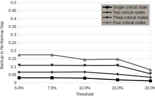
6.1 Increase on distance values, obtained by the heuristic, when backup is provided. . . 32

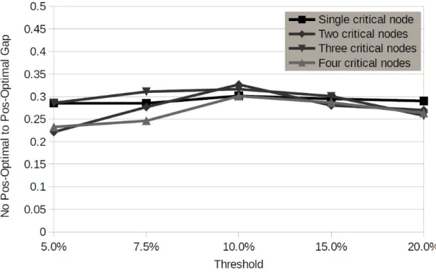
6.2 Decrease on distance values, obtained by the heuristic, when pos-optimal procedures are applied. Backup is being provided. . . 33

6.3 Backup provisioning vs vehicle from depot time radio. . . 34 A.1 Passive infrared. . . A-1 B.1 PIR setup . . . B-4 B.2 Gateway communication . . . B-5

(11)

Nomenclature

6LoWPAN IPv6 over Low power Wireless Personal Area Networks

CDT C/C++ Development Tooling

CI CodeIgniter

CRUD Create, Read, Update and Delete

CSS3 Cascading Styles Sheets version 3

DARP Dial-a-ride Problem

FSM Finite State Machine

GIS Geographical Information System

GPRS General Packet Radio Service

GPS Global Positioning System

GSM Global System for Mobile

HPP Hamiltonian Path Problem

HTML5 HyperText Markup Language version 5

IETF Internet Engineering Task Force

IDE Integrated Development Environment

IPv4 Internet Protocol version 4

IPv6 Internet Protocol version 6

ITS Intelligent Transportation Systems

LED Light Emitting Diode

MAC Media Access Control

MDVRP Multi-Depot Vehicle Routing Problem

MVC Model-View-Controller

OVRP Open Vehicle Routing Problem

PDT PHP Development Tools

PIR Passive Infrared

PHP PHP Hypertext Preprocessor

RFC Request for Comments

RFID Radio Frequency Identification

RSUs Road side units

UN United Nations

UTCS Urban Traffic Control System

UTGS Urban Traffic Guidance System

UTN Urban Transportation Network

UTS Urban Transportation System

V2R Vehicle to Road Side

V2V Vehicle to Vehicle

(12)

VRP Vehicle Routing Problem WSN Wireless Sensor Networks

(13)

List of Publications

1. Carvalho, N. and Sch¨utz, G. and Correia, N. “Vehicle Routing with Backup Provi-sioning Using Wireless Sensor Infrastructure”, IEEE International Conference on Connected Vehicles and Expo 2014.

2. Carvalho, N. and Sch¨utz, G. and Correia, N. “On the Planning of Vehicle Routing with Backup Provisioning Using Wireless Sensor Technologies”, IEEE Intelligent Transportation Systems Transactions and Magazine (submitted article).

(14)

C H A P T E R

1

Introduction

With today’s technologies, demographic changes leading people to larger cities and the permanent concern with our natural resources, such as energy, it is inevitable that we seek ways to improve our cities. Several steps are being given forward. In Boston, USA, converting street lighting to LEDs (Light Emitting Diode) led to a $2.8 million saving per year with only 40% light converted [1]. In Coimbra, Portugal, the trend is similar as LEDs were adopted for street lighting as an energy saving measure. Besides this, car companies are equipping their vehicles with parking sensors, cameras, luminosity sensors to turn on headlights.

1.1 Motivation

Sensors are a key issue in intelligent environments, and currently we are faced with smaller, cheaper and low-power sensors, which can be deployed in many places. These sensors have limited processing power, storage and battery, low bandwidth and short range. The possibility of organizing these sensors into networks, along with the Internet, brought several opportunities such as environment monitoring, battle field surveillance, among others [2, 3]. Many governments are looking to transform their cities into smart cities. The goal for most cities is to manage and probe their infrastructures and resources efficiently for environmental sustainability and better urbanization development, among others. As major cities continue to grow, these are forced to become “smarter”.

According to United Nations (UN) forecast in 2050 70% of world population will live in cities (currently there are about 50%) [4] and there will be about 27 cities with more than 10 million people. Beside this, the human behaviour is leading to a breakpoint on world’s natural resources. Global warming, air pollution, among others are the top challenges and the priority of cities (nowadays about 95% of cities still dump raw sewage into their waters). This forces the improvement of cities and urban infrastructures, so that society can deal with such growth of people in cities. This improvement requires tools, which can be related with:

(15)

1.1 Motivation ii) Management; iii) Operation.

Planning tools based on merged information about human behaviour are required to aid allocation of resources, as land, water, roads, transportation, sewage, among others. Concerning management concerns these are related with the coordination of infrastruc-tures to plan interventions (such as build and maintain roads, cables and power lines). Operation can be executed depending on the demand and/or based on historical usage, like power capability (amount of power/energy on the lines) during holidays like Christ-mas. These tools could be applied, for example, to traffic, signalling and traffic lights. Information gathered could reduce the impact of future demands as well as the amount of time spend in traffic.

Transportation networks is another area where such improvement tools could be use-ful. Each day, we concern ourselves with being efficient with our resources and increas-ingly look for ways to improve productivity. One main concern is the time spent, each day, in transportation networks. It’s reduction is essential in order to become more effi-cient. As the population of larger cities increases, good urban transportation system must, therefore, be provided. Wireless sensor networks are expected to help on the planning of Urban Transportation Systems (UTS) [5, 6] and even aid blind in UTS [7]. The core prob-lem is its complexity as there are numerous variables such as weather conditions, time, accidents, which makes it virtually impossible to predict the behaviour of traffic flow and hampers urban transportation scheduling planning.

As new technologies emerge it is inevitable that we look for ways to improve our ur-ban transportation networks. The decisions that might lead to such improvements mainly depend on the provisioning of timely information and monitoring tools. Thus, intelligent transportation systems(ITS) are now under strong research. These systems are endowed with communication capabilities for data transmission between vehicles (V2V) and be-tween vehicles and roadside access points (V2R), also called road side units (RSUs). ITS are seen as key technologies for road safety improvement, congestion avoidance using op-timal routing and scheduling, and for the improvement of quality of service experienced by users (both drivers and customers) [8]. This thesis falls within ITS as explained in the following section.

(16)

1.2 Contributions

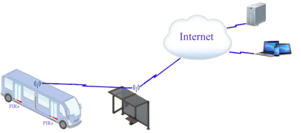
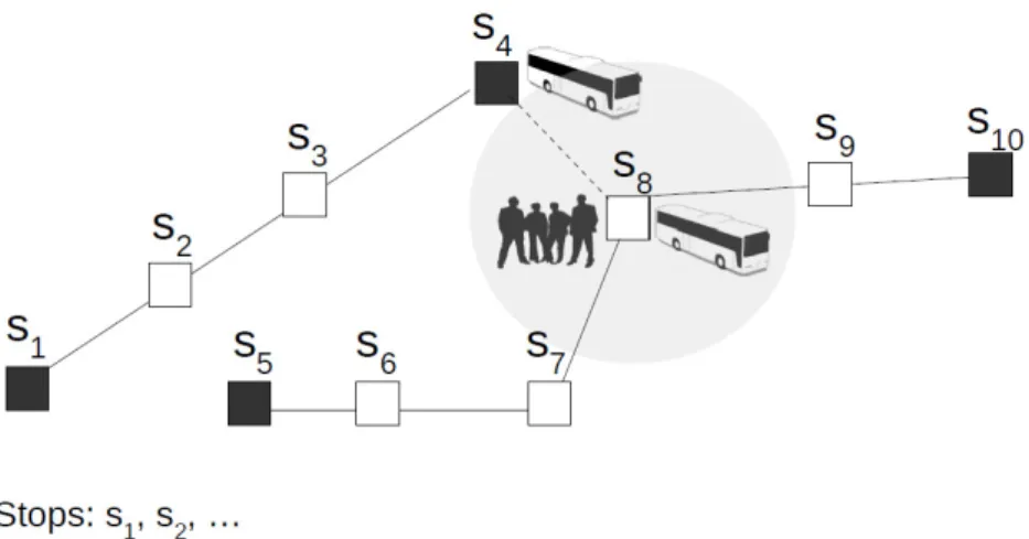
The present thesis explores ways of improving transportation networks. We try to achieve this by planning vehicle routes that include the possibility of reacting to the overload-ing/overcrowding of vehicles in certain stops. This vehicle routing with backup provision-ing paradigm is based on the availability of vehicle load information in real time, which can be captured using wireless sensor technologies, as illustrated in Figure 1.1. It is as-sumed that vehicles incorporate two passive infrared (PIR) sensors at each entrance/exit, to sense movement and determine direction. Having such information available, a vehicle finishing its route in the neighbourhood may pickup more customers in case of over-load. This is illustrated in Figure 1.2, which includes two routes r1 = {s1, s2, s3, s4} and

r2 = {s5, s6, s7, s8, s9, s10}. Stop s8 is considered a critical one that occasionally gets

congested and, therefore, routes have been planned so that there is a vehicle finishing its route near, being able to get fast to s8 and pick up more customers. In this example,

the vehicle finishing route r1 at stop s4 is the one moving to s8. Time for backup to

ar-rive should not exceed a certain time threshold. Note that, once planned, routes remain unchanged and route extensions (or backup) are only activated in case of overload.

Figure 1.1: Vehicle to roadside access point example.

This vehicle routing with backup provisioning paradigm allows sustainable urban mo-bility with efficient use of resources, since an agile and adaptable fleet with not so big fleet elements and less schedules per day can be adopted, while improving the quality of ser-vice experienced by users.

In summary the benefits of this approach will be:

• Sustainable urban mobility: The availability of vehicle load information and reac-tive response in case of overload will allow sustainable urban mobility;

(17)

1.2 Contributions

Figure 1.2: Illustration of vehicle routing problem with reactive response to overload.

(energy, infrastructure, and vehicles). An agile and adaptable fleet with not so big fleet elements and less schedules per day can be adopted;

• Improve quality of service experienced by users: Fast response to overload allows user waiting times to be reduced.

Besides route planning, including backup provisioning, a monitor tool is also devel-oped so that the amount of people at urban transportation is tracked. This will allow companies to optimize their route plans, and schedules, considering traffic issues like delays and traffic flow at different hours, in order to achieve better tradeoff between cus-tomers satisfaction and resources used (e.g. energy and fuels wastes). For cuscus-tomers, the objective is also to use the collected data to inform them the time of arrival, free seats etc, available in train stations, bus stops or even through phones or any Internet connected device.

In summary, the contributions of this thesis include:

• Proposal of a vehicle routing with backup provisioning approach for urban trans-portation planning;

• Mathematical formalization of the problem;

• Proposal of heuristic algorithm using greedy strategy;

• Pos-optimal procedures to be incorporated into heuristic algorithm;

• Analysis of the benefits of incorporating backup provisioning into vehicle routes; • Monitoring tool.

(18)

1.3 Organization

In Chapter 2 we analysed the state of the art in vehicle routing and work done using WSNs in monitoring and tracking. At Chapter 3 the monitoring tool developed is discussed. Among other things, this tool will allow the occupation of vehicles to be followed in real time, and critical stops to be detected. With this information the routes of vehicles can be planned with backup provisioning in mind, which is done in Chapter 4. At Chapter 5 we propose a heuristic algorithm to solve the routing problem in question. Since our algorithm uses a greedy methods and they can produce not so good results, because a solution can be a local optimum, in Section 5.2 we propose pos-optimal procedures to improve our algorithm performance. In Chapter 6 we analyse the results obtained. We discuss our results, draw conclusions and plan future work at Chapter 7.

(19)

C H A P T E R

2

State of the art

2.1 Transportation networks

Efficient transportation of goods and persons are problems that have been studied over the last 50 years. Thousands of papers have been written on several variants of these opti-mization problems. The most well known are the vehicle routing problem (VRP) and the dial-a-ride problem(DARP). In the classical VRP the concern is to find a set of optimal routes for a fleet of vehicles, based at the depot, to satisfy the demand of geographically dispersed customers at the minimum total travelling cost, while satisfying vehicle capac-ities. A lot of variants of the stated problem exists: considering time-windows, pick up and delivery customers, different vehicles, multiple depots, and so on [9]. In DARP the goal is to design vehicle routes and schedules for users specifying pick-up and drop-off requests between origins and destinations. A set of minimum cost vehicle routes, capable of accommodating as many users as possible under a set of constraints, will be the output [10].

More recently, a variant of the classical VRP, called OVRP, attracted the attention of practitioners and researchers. In this case vehicles are not required to return to the depot after serving the last customer on a route [11]. This usually arises in cases where indus-tries do not own a vehicle fleet, or their private fleet is inadequate to fully satisfy customer demand, and distribution services (or part of them) are either entrusted to external contrac-tors or assigned to a hired vehicle fleet. In these cases, vehicles are not required to return to the central depot after their deliveries have been satisfied. The main difference between VRP and OVRP is that in VRP the routes are Hamiltonian cycles and in the OVRP the routes are Hamiltonian paths originated at the depot and ending at one of the customers, so the shortest Hamiltonian Path Problem (HPP) with a fixed source node has to be solved for each vehicle in the OVRP. The shortest HPP is known to be NP-hard since an instance of the HPP can be converted into an instance of the traveling salesperson problem that is known to be NP-hard. Consequently, the OVRP is also an NP-hard problem. Our prob-lem, as far as known not yet discussed in the literature, is a variant of the OVRP applied to the transportation of persons, considering multiple depots and having the possibility of

(20)

2.2 Wireless sensor networks

backup provision to certain critical stops, having high number of customers.

2.2 Wireless sensor networks

Wireless sensors have been used for monitoring and tracking in several areas: health and wellness, power supply, automated machinery monitoring, traffic monitoring, tracking of human and animals. Concerning its use in the context of traffic and urban transportations, wireless sensors have been used to improve traffic control in large cities [12], collect information of passenger volume [5], to plan traffic signals giving priority to buses [6], provide optimal routes in real-time [13], and even aid blind [7]. The system in [13], is useful as an information system and coordination between different transportations. In [5] the system used for data gathering is discussed but no further planning using such information is done. Here we go further and use the gathered data for vehicle route planning with backup provisioning.

There are several detection/tracking sensor types of thermal signature and/or light changes. The authors in [14] present the weaknesses of several approaches. For our problem we have decided to use PIR, leaving aside other type of sensors like photoelectric sensor that, depending on the type, may requires two points to install, a sensor and a receptor.

We can divide Wireless Sensor Networks (WSNs) into two categories: Monitoring and Tracking. In Monitoring we can include, among others, health and wellness, power supply, automated machinery monitoring, traffic monitoring. In tracking applications we can include object tracking, animals (like ZebraNet [15]), human (PinPtr [16]), vehicles, objects (MAX [17]).

There are several proposals for tracking and monitoring, including cluster based archi-tectures [18, 19], tree-based approaches [20, 21], and Prediction-based Mobility Adaptive Tracking (P-MAT) [22]. All previous proposals are based on the high accuracy of track-ing while minimiztrack-ing the power consumption of the WSN. Some work focus on energy conservation [20] or the tradeoff between energy efficient vs. accuracy of target [23].

Concerning Urban Traffic Systems, which are related with the work developed in this thesis, these have been discussed in [12, 24, 25, 26]. In [12] a city traffic system was proposed for traffic flow control using a WSN, which was expected to deal with the stochastic nature of traffic flows. The Urban Traffic Control System (UTCS) and Urban Traffic Guidance System (UTGS) at China were analysed in [25] and it is stated that these are expected to be the most efficient possible, with effective techniques to reduce traffic congestion, making driving more secure, easier and more comfortable.

A fleet management system (FMS), using Global System for Mobile (GSM) and Gen-eral Packet Radio Service(GPRS) was discussed in [27], with the advantage of GPS to track in real time the company fleet. A Radio Frequency Identification (RFID) was one of

(21)

2.2 Wireless sensor networks

the techniques used in [28, 29] to identify the fleet along with Geographical Information System(GIS).

For human and movement detection in [30] they used the received signal strength indicator (RSSI) between stationary 2.4 GHz smart outlets. In [31] PIR sensors were used for multiple human tracking, while [24, 26] used PIR to detect human intruders. Our job is not to detect intruders, but we must be able to count how many persons enter and exit the urban transportation. The work to be developed here can be seen as fitting into both tracking and monitoring systems:

• Tracking: PIR will be used to detect direction in transportation entries.

• Monitoring: Data collected and stored within a monitoring tool, at edge devices. The PIRs we will be using have similar characteristics to the ones used in [24, 26]. Have a detection angle of 110◦, to be more exact 93◦ horizontally and 110◦ vertically, have a range of 10 meters and can detect moving objects that feature a temperature differ-ent from the environmdiffer-ent (such as humans).

(22)

C H A P T E R

3

Monitoring tool

3.1 Development tools and geographical information

soft-ware (GIS)

In this thesis the Eclipse Integrated Development Environment (IDE) was used with PHP Development Tools (PDT) and C/C++ Development Tooling (CDT). The PDT was used to build the monitoring tool and the CDT to program the sensors.

The monitoring tool was developed mainly using PHP Hypertext Preprocessor (PHP), HyperText Markup Language version 5 (HTML5), Cascading Style Sheets version 3 (CSS3) and Javascript. In any Web tool there are two sides: server-side and client-side. The server is responsible for serving the pages and several programming languages can be used at the server-side, like PHP, C#, among others. The client requests pages from the server and displays them to the user. Sometimes user interaction and dynamically gener-ated content is needed and, therefore, a client-side language like Javascript is needed.

In this thesis the CodeIgniter (CI) is also used to develop the monitoring tool [32]. CI uses model-view-controller pattern (MVC).

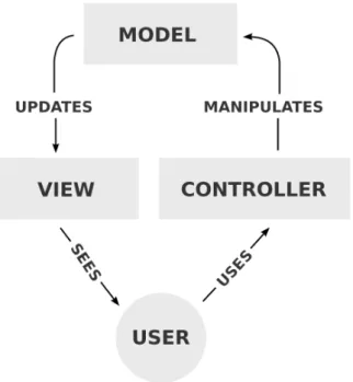
Most PHP frameworks use the model-view-controller pattern (MVC), but there are differences in what they are capable of [33], development speed, learning curve, code generation, among others. The Model is the application object, the View is its screen presentation, and the Controller defines the way the user interface reacts to user input. The MVC pattern diagram is shown in Figure 3.1. The main advantages of using such pattern is the increased flexibility and code reuse. Our previous experience allow us to work with some PHP Frameworks CakePHP, Yii and CodeIgniter (CI) [32]. From these three CakePHP [34] and Yii [35] have the ability to generate code, for example, creation of Create, Read, Update and Delete (CRUD).

All these frameworks need a well designed and implemented database. In the case of CakePHP and Yii the code generated is based on the database design so any database change during development (e.g. new feature that requires a database change on a already build table) may force us to rebuild the code, and any changes made on those models, views or controllers may be lost or recoded. Since the tool being developed in this thesis

(23)

3.1 Development tools and geographical information software (GIS)

will be constantly evolving, depending on evolving needs, the CI framework has been chosen.

Figure 3.1: MVC pattern diagram.

(24)

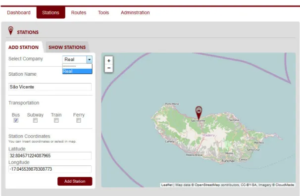
Figure 3.3: Monitoring tool - Adding stations.

Along with CI, a free Geographical Information Software (GIS) [36], the Leaflet, has also been used. GIS “integrates hardware, software, and data for capturing, managing, analysing, and displaying all forms of geographically referenced information” [37]. GIS is usually seen as a map, but it can make spatial information analysis and data editing, and it can perform basic geoprocessing tasks, such as routing and map image display.

(25)

In our case this will allow us to add stations/stops, collect data like distance between stations/stops, display all necessary information, among others.

Figure 3.2 shows the home page of the developed tool, including several stations. The main goal for this tool is constant evaluation. We need stations to be inserted in the platform and there are two ways of doing it:

i) upload a file with stations name and coordinates;

ii) inserting them directly in the platform shown in Figure 3.3.

In Figure 3.4 routes are built by selecting a name for the route, then stations are incor-porated, mandatory stations are set, and time between stations or maximum time to reach mandatory stations can be defined.

(26)

3.2 Infrastructure and data collection

In this thesis the iSense Security Modules [38], referred from now on as nodes, have been used to capture data while the Coalesenses Gateway Module, from now on referred as sink or gateway, have been used to forward data to the monitoring tool. The main reason to work with these sensors is the possibility of setting up them according to our needs, and code/parameter change possibility at deployment time, like identification numbers for nodes.

We choose to implement our communications using IPv6 rather than IPv4. IPv4 al-lows us to allocate 232 _{addresses, but with the constant grow of devices with}

communi-cation needs it is mandatory to implement IPv6 that allows us to have 2128 _{IP numbers.}

Internet Engineering Task Force (IETF) published, in December 1998, their specification of IPv6 [39] and several updates to this Request for Comments (RFC) were published in the last years, and most devices work now with both IPv6 and IPv4 stacks. The use of both stacks is due to the high cost of changing all IPv4 devices, those that do not support IPv6. There is no easy way for this transaction, and it is being done progressively with equipments incorporating both stacks.

Our first step was to implement IPv6 communications between the nodes and the sink or gateway. The protocol stack implemented at our devices was the IPv6 over Low power Wireless Personal Area Networks (6LoWPAN), which allows an easier integration of nodes in the Internet and allows similar management to standard IP-based networks. Our nodes and sinks have limited power, short range and low bandwidth, so it is important to choose a low power stack. We have reduced the sensor’s area of action to a narrow beam, more specifically from the default 110◦ to 20◦-30◦. We have developed some experiences to see the behaviour of the sensor and gateway, regarding communications, IPv6 addresses assigned, node identification and people counting.

The gateway was configured to assign IPv6 addresses to all discovery nodes, and once the nodes receive an IPv6 address they automatically store the IPv6 address of the gateway allowing them to send their data over to the gateway. Note, however, that a gateway could assign IP addresses to nearby vehicles, which might not be acceptable. Therefore, the IP assignment should take MAC addresses (of nodes inside the same vehicle as the gateway) into consideration. That is, the assignment of IP addresses, done by the gateway, should be restricted to the nodes inside the same vehicle. This can be easily achieved since our sensors allow on site configuration. The data send by nodes was:

• node Identification; • node counting.

(27)

simple and easier to manage solution was found. Nodes identification was composed by two parts:

• Transportation Identification: An unique number identifying each transportation; • PIR Identification: A number between 1 and 4 identifying each PIR sensor, PIR 1

and 2 at the entrance and PIR 3 and 4 at the exit. Even numbers placed on the inside and odd numbers placed more at the outside, as showed in Figure 3.5.

Figure 3.5: Sensor application in a bus.

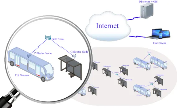
The Figure 3.5 shows an example of where the sensors will be placed, inside a bus, where the red area is the coverage of the PIR sensor. Figure 3.6 shows how the sensors will connect to the Internet. Data is sent to the sink and this one is responsible for transmitting data through the Internet. Sink nodes are connected to the Internet with an Ethernet cable.

(28)

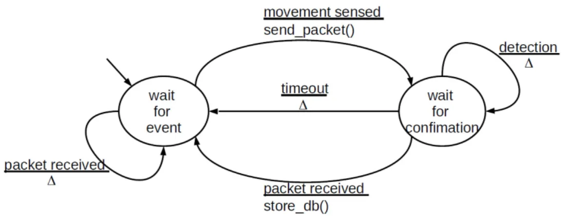
Figure 3.7: FSM diagram for each sensor node of dual implementation.

The infrastructure assumed in vehicles includes a dual PIR implementation at each entrance/exit. This dual PIR is used to control the direction of people passing. The finish state machine(FSM) diagram of each PIR node of such dual implementation is shown in Figure 3.7. The diagram is the same for both nodes.

While in the “wait for event” state, node i might sense movement of people and, in this case, a packet is sent to its neighbour j. After sending this packet the node waits for a confirmation from node j. When such confirmation arrives a i − j movement is stored at a remote database, using WiFi or WiMAX, and the node enters in “wait for event” state again. When waiting for confirmation another detection may occur, and in this case no action is taken to avoid counting the same person many times. If timeout occurs, meaning that the person probably walked back, also no action is taken and the node enters in “wait for event” state. While in the “wait for event” state, a node i might receive a packet from its neighbour j (meaning that it has detected movement) asking for a confirmation. Node i remains waiting because a movement must be sensed by i for a packet to be sent to j, which will serve as confirmation to j. Upon receiving such packet, its neighbour (which is in “wait for confirmation” state) will send a j − i movement for storage in the remote database.

(29)

3.3 Improvement of transportation networks

The development of a tool to capture urban transportation information allows the opti-mization of such networks. In case different transportation networks are integrated, or information about other networks is available, integrated policies may also be outlined. A final goal is to develop mathematical models and/or algorithms based on the collected data, which might include load, time of arrival to collecting nodes, or other. The problems that can be addressed include the improvements of:

• routes • schedulings

• coordination between different transportations

These may include proactive or reactive strategies. In this thesis scheduling and coordi-nation between different transportations is not handled.

(30)

C H A P T E R

4

Problem formalization

4.1 Problem definition

In the following it is assumed that routes are planned without mention to their sched-ules. The resulting routes can then be adopted many times a day according to the needs, requiring further assignment of schedules and drivers.

4.1.1 Notation and definitions

In the definitions discussed next R is a given set of routes that must be planned, each route initially having just the source and one or more mandatory stops, and S is a given set of stops/locations that must be incorporated into the routes for them to be visited. A set of stops requiring backup, in case of overload, is given by B ⊂ S.

Definition 1 (Route) A route r ∈ R can be seen as a path that initially has a starting point,src(r), and a set of mandatory stops, Mr _{⊂ S. There are at least two mandatory}

stops,src(r) and another location that might end up being the destination or not. Other stops will be inserted during route construction. The final destinationdst(r) can be any stop, mandatory or not.

Definition 2 (Mandatory Stop) A mandatory stop s ∈ Mris a location point that must be visited by the vehicle of route r. A mandatory stop s has a time window info i(s) = {s0_{, ∆(s}0_{, s)} associated with it, which indicates the maximum allowed time from the}

pre-vious locations0 ∈ Mr_{, also mandatory and to be included in the route, until}_{s ∈ M}r_.

The extra stops to be inserted in a route, during route construction, can not violate the time window associated with mandatory stops.

The i(s) = {s0, ∆(s0, s)} pair for a mandatory stop s basically expresses the following: ”if the departure from s0 is done at time ∆s0, or after, the arrival to s must be no later than

(31)

4.1 Problem definition

∆s0+ ∆(s0, s)”. The insertion of mandatory stops, with a reference to a previous stop and

time window, allows round trips or trips with specific connection points to be planned.

Definition 3 (Stop) Any stop s ∈ S, mandatory or not, is a location point that must be visited by at least one route. A pair of stops(si, sj) has a cost t(si, sj) associated with

it that is basically the estimated time when going from si directly to sj. If s ∈ B then

backup must also be provided for a reactive response in case of overload.

Definition 4 (Backup) A backup for a critical stop s ∈ B can be supplied by any vehicle reaching its destination stop at some place near, and able to reachs before a specified time threshold T . That is, the backup for s, denoted by b(s), will be a route, b(s) ∈ R, whose vehicle will have to make an extra traversal from dst(b(s)) to s in less than T , a threshold for the maximum allowed time for backup to arrive.

Note that every stop must be visited at least once. A stop may be visited more than once because routes will be built having backup for critical stops into consideration. That is, routes might be extended to provide backup, leading to more visits at some stops. However, this is expected to be better than increasing scheduling and number of vehi-cles/drivers. A minimum number of stops per route is not imposed since it is assumed that the set of routes to be planned is adequate to the fleet and region covered. Routes with few stops can always be eliminated from the final solution.

Having the previous notation and definitions in mind, our route planning problem can be defined as follows. This problem is called here vehicle routing with backup provisioning (VRwBP).

Definition 5 (VRwBP) Given a set of routes R, each route r ∈ R with a reference to a set of mandatory stopsMr _{with time constraints, a set of stops}_{S that need to be visited}

and a set of critical stopsB ⊂ S requiring backup, insert stops into routes while not vio-lating time constraints, and ensuring backup to critical stops, in less than a time threshold T .

Please note that routes are to be planned without taking into consideration schedule assignment. After determining the routes, these can be adopted many times a day ac-cording to the needs and, therefore, further schedule/fleet/drivers planning is required. These issues are determinant for the availability of a backup vehicle when overcrowding is detected.

(32)

4.2 Mathematical formalization

To find the optimal solution for the VRwBP problem we proceed with its mathematical formalization and discussion. This will also allow for a deep understanding of the prob-lem, allowing adequate procedures to be used by the heuristic algorithm proposed in the next section. In the following formalization it is assumed that t(si, sj) = ∞ if si = sj.

Before going into the formalization let us summarize the known information:

R Given set of routes to be planned, initially with source and one or more mandatory stops.

S Given set of stops to be visited at least one time. Mr _{One or more mandatory stops in route r.}

B Set of stops requiring backup.

src(r) Source for route r.

dst(r) Final destination for route r.

s0, δ(s0, s) Mandatory stop time window information. t(si, sj) Cost between stops siand sj.

The variables that need to be found are:

ξ_sr_i One if route r ∈ R selects stop si ∈ S to become its final destination,

dst(r), zero otherwise.

υr_s_i_,s_j One if route r ∈ R includes going directly from stop sito sj ∈ S, zero

otherwise. κr,s

si,sj When ensuring that the time window associated with mandatory stop s

of route r is non violated, this accounts the time items flowing from si

to sj ∈ S. – Objective Function: Minimize X r∈R X si∈S X sj∈S t(si, sj) × υrsi,sj (4.1)

This avoids unnecessary long routes and minimizes the number of visits to stops. – Building routes: X sj∈S:t(si,sj)6=∞ υ_sr i,sj = 1, ∀r ∈ R, si = src(r) (4.2) X sj∈S:t(si,sj)6=∞ υ_sr i,sj − X sj∈S:t(sj,si)6=∞ υ_sr j,si = (−1) × ξ r si, ∀r ∈ R, ∀si ∈ S\{src(r)} (4.3)

(33)

X

s∈S

ξr_s = 1, ∀r ∈ R (4.4)

Expression 4.2 forces routes to emanate from the source src(r), expression 4.3 im-poses the flow conservation law to routes and expression 4.4 forces the existence of a final destination stop. – Mandatory stops: X sj∈S:t(si,sj)6=∞ υ_sr_i_,s_j + X sj∈S:t(sj,si)6=∞ υ_sr_j_,s_i ≥ 1, ∀r ∈ R, ∀si ∈ Mr (4.5)

The vehicle of a route r is forced to arrive/depart from every mandatory stop of that route. – Ensuring backup: minr∈R{ X sj∈S ξ_sr_j× t(sj, si)} ≤ T, ∀si ∈ B (4.6)

where T is a threshold for the maximum allowed delay for backup to arrive. Expression 4.6 may be expanded to a set of linear expressions.

– Visited times: X r∈R X sj∈S:t(si,sj)6=∞ υ_sr_i_,s_j +X r∈R X sj∈S:t(sj,si)6=∞ υ_sr_j_,s_i ≥ 1, , ∀si ∈ S (4.7)

Constraints 4.7 state that every stop must be visited at least once. – Time windows: κr,s_s0 = ∆(s 0 , s), ∀r ∈ R, ∀s ∈ Mr∧ s 6= src(r), {s0, ∆(s0, s)} ∧ s0 ∈ Mr _(4.8) κr,s_s i − t(si, sj) + K × (1 − υ r si,sj) ≥ κ r,s sj, ∀r ∈ R, ∀s ∈ Mr_{, ∀s} i, sj ∈ S (4.9)

(34)

κr,s_s ≥ 0, ∀r ∈ R, ∀s ∈ Mr

(4.10) where K is a big time constant. These constraints ensure that the time windows associated with mandatory stops, i.e. the maximum allowed time from the previous mandatory stop, are not violated. For this purpose, considering a route r and mandatory stop s with time window {s0, ∆(s0, s)}, the stop s0is assumed to have a ∆(s0, s) time in it that will vanish as the route is traversed toward s (can be seen as time items that will be deposited in intermediate stops from s0 to s). This is what constraints 4.8-4.9 do. Expression 4.10 ensures that the stops used to control the non violation of time windows are the ones at the routes being built.

– Non-negative assignments

κr,s_s_i _{∈ R; υ}_sr_i_,s_j, ξ_sr_i ∈ {0, 1}. (4.11) A minimum number of points per circuit is not imposed since it is assumed that the set of circuits to be planned is adequate to the fleet and region covered. Circuits with few stops can always be eliminated at solution is provided.

As previously said, this problem can be seen as a variant of the OVRP applied to the transportation of persons, considering multiple depots and having the possibility of backup provision to certain critical stops. In OVRP vehicles are not required to return to the central depot after their deliveries have been satisfied [11]. The main difference be-tween VRP and OVRP is that in VRP the routes are Hamiltonian cycles and in OVRP the routes are Hamiltonian paths originated at the depot and ending at one of the customers, so the shortest Hamiltonian path problem (HPP) with a fixed source node has to be solved for each vehicle in the OVRP. The shortest HPP is known to be NP-hard since an instance of the HPP can be converted into an instance of the traveling salesperson problem that is known to be NP-hard. Therefore, the OVRP, and consequently our problem, are also NP-hard problems. For this reason the development of an efficient heuristic approach is needful. This will be done in the following Chapter.

(35)

C H A P T E R

5

Heuristic algorithm

5.1 The algorithm basis

The heuristic approach proposed in this section has two main steps:

• Framework route building: Here the concern is to build the basis framework of routes, where all stops are visited while not violating time window constraints. • Extension for backup inclusion: After building the basis framework, routes are

ex-tended for backup provision to be ensured.

To evaluate the possibility of inserting stops in specific routes, neighbourhood information around stops is built. Neighbourhood information is associated with consecutive pairs of mandatory stops, to evaluate the possibility of inserting an extra stop between them. Please note that given i(s) = {s0, ∆(s0, s)} info for a mandatory stop s will change when stops are permanently inserted into routes. Initially, when s is inserted after s0, t(s0, s) is subtracted from ∆(s0, s) so that it stores the time margin left for further insertions of stops. Whenever a stop is permanently inserted between s0and s this will be updated.

5.1.1 Route framework

When building the basis framework of routes the following variables are required: η_(sr

i,sj)Neighbourhood for the pair of mandatory stops si and sj ∈ M

r _{of route}

r ∈ R. Used to evaluate the possibility of inserting an extra stop between si

and sj.

ωr

(si,sj)Cost of inserting a specific stop between the pair of mandatory stops siand sj

of route r ∈ R. Used when building neighbourhoods. θ Specific subset of all the neighbourhoods.

Neighbourhood elements are (sk, ϕ) pairs, where sk is a potential extra stop and ϕ the

time margin left if sk is to be inserted. The output will be:

Lr List of stops for each route r ∈ R. dst(r) Destination stop for each route r ∈ R.

(36)

5.1 The algorithm basis

Building the route framework includes inserting mandatory stops first and then non-mandatory. While retrieving from the pools of stops Mr and S, and inserting in the ordered Lrlists, the time windows are updated to stay with the time margin left. During the following discussion an example is used, for illustration, that considers the stops in Figure 1.2.

• Inserting mandatory stops: Routes start by having mandatory stops.

1 for each r ∈ R do

2 /*list of stops for route r starts with source*/; 3 Lr = {src(r)};

4 s = {s ∈ Mr : i(s) = {src(r), ∆(src(r), s)}}; 5 repeat

6 /*mandatory stop is s*/; 7 s0 = s;

8 /*insert mandatory stop*/; 9 Lr ← s0;

10 /*determine next mandatory stop*/; 11 s = {s ∈ Mr : i(s) = {s0, ∆(s0, s)}}; 12 /*update margin left*/;

13 ∆(s0, s) = ∆(s0, s) − t(s0, s); 14 until s == N U LL;

15 /*destination is last stop inserted*/; 16 dst(r) = s0;

17 end

• Inserting non-mandatory stops: Here the neighbourhoods are built first and then non-mandatory stops are inserted using this info. Stops not inserted in any route will be attached at the end of routes.

– Neighbourhood formation: Neighbourhood info is built for each pair of consec-utive mandatory stops.

(37)

1 /*neighbourhoods start empty*/; 2 for each r ∈ R do

3 for each pair of consecutive mandatory stops (s0_j, s_j) ∈ Lrdo 4 η_(sr0

j,sj)= {};

5 end 6 end

7 /*fill neighborhood info*/; 8 for each r ∈ R do

9 for each pair of consecutive mandatory stops (s0_j, sj) ∈ Lrdo 10 for each sk∈ {S −S_r∈RMr} do

11 /*cost of inserting s_kbetweens0_j andsj*/; 12 ω_(sr0 j,sj)= t(s 0 j, sk) + t(sk, sj) − t(s0j, sj); 13 if ω_(sr0 j,sj) < ∆(s 0 j, sj) then 14 /*time margin*/; 15 ϕ = ∆(s0_j, s_j) − ωr_(s0 j,sj); 16 /*neighbourhood is increased*/; 17 η_(sr0 j,sj)← {(sk, ϕ)}; 18 end 19 end 20 end 21 end

– Insertion using neighbourhood info: Insert first the stops included in a single neighbourhood and then stops included in many neighbourhoods according to time margins left.

(38)

1 for each sk ∈ {S −S_r∈RMr} do

2 /*extract neighbourhood elements referring to s_k*/; 3 θ = {(s, ϕ) ∈S_r∈R,s

j∈Mrη

r

(s0_j,sj) : s = sk};

4 /*number of times s_kis included in neighbourhoods*/; 5 if |θ| == 1 then

6 /*extract place where skmust be inserted*/; 7 {r, (si, sj)} = {r, (si, sj) : θ ⊂ ηr_(s0

j,sj), ∀r ∈ R, (si, sj) ∈ L

r_}; 8 /*insert s_kinto router between stops siandsj*/;

9 InsertInBetween(Lr,(si, sj),sk); 10 /*update time window margin*/;

11 ∆(s0_j, sj) = ∆(s0j, sj) − [t(si, sk) + t(sk, sj) − t(si, sj)]; 12 end

13 end

14 for each sk ∈ {S −Sr∈RMr} do

15 /*extract neighbourhood elements referring to sk*/; 16 θ = {(s, ϕ) ∈S_r∈R,s

j∈Mrη

r

(s0_j,sj) : s = sk};

17 /*number of times skis included in neighbourhoods*/; 18 if |θ| > 1 then

19 /*extract place where s_kmust be inserted; the one leaving the largest margin*/; 20 {r, (s_i, s_j)} = {r, (s_i, s_j) : (s_k, ϕ) ∈ ηr_(s0

j,sj)∧ (sk, ϕ) =

argmax(sk,ϕ0)∈θ{ϕ

0_{}, ∀r ∈ R, (s}

i, sj) ∈ Lr}; 21 /*insert s_kinto router between stops siandsj*/; 22 InsertInBetween(Lr,(si, sj),sk);

23 /*update time window margin*/;

24 ∆(s0_j, sj) = ∆(s0j, sj) − [t(si, sk) + t(sk, sj) − t(si, sj)]; 25 end

26 end

– Remaining stops: Stops not inserted at previous steps will be inserted at the end of current routes.

1 for each s_k ∈ L/ rdo

2 /*Select route whose destination is more near s_k*/; 3 r = argmin_r∈R{t(dst(r), s_k)};

4 /*insert stop*/; 5 Lr ← sk;

6 /*destination is last stop inserted*/; 7 dst(r) = s_k;

(39)

5.1.2 Backup inclusion

When determining how backup is to be provided the following variables are required: ζs Set of routes that can provide backup to s ∈ B.

δ Time it takes for backup to arrive.

ϑ List of stops resulting from a shortest path calculation. The output will be:

b(s) Backup for every stop s ∈ B.

Lr _{Final list of stops for every route r ∈ R, after extending if necessary.}

dst(r) Final destinations for every route r ∈ R, after extending if necessary.

The following code is used to extend the route framework in order to incorporate backup provision, where T is a threshold for the maximum allowed time for backup to arrive, as mentioned in Section 4.1.1.

1 for each s ∈ B do

2 /*initially list of potential backup providers is empty and time for backup arrival is a

big value*/;

3 ζs= {}; 4 δ = ∞;

5 for each r ∈ R do

6 if t(dst(r), s) ≤ T then

7 /*after finishing route r, vehicle is able to arrive to s before T */; 8 ζs= ζsS{r};

9 end

10 if t(dst(r), s) ≤ δ then

11 /*time for backup arrival is updated*/;

12 δ = t(dst(r), s);

13 b(s) = r;

14 end 15 end

16 if ζs== ∅ then

17 /*in next step do not consider direct links with cost/time higher than T */; 18 ϑ=ShortestPath(source = dst(b(s)), destination = s); 19 while t(dst(b(s)), s) > T do 20 dst(b(s))=RemoveHead(ϑ); 21 Lb(s) ← dst(b(s)); 22 end 23 end 24 end

The above procedures plan routes without taking into consideration schedule assign-ment. After determining the routes, these can be adopted many times a day according to the needs and, therefore, further schedule/plan/drivers planning is required.

(40)

5.2 Improvements to algorithm

Since our algorithm uses greedy methods and they can produce not so good results, be-cause a solution can be a local optimum, we choose to apply pos-optimal procedures. After the routes have been constructed the following pos-optimal local search procedures are executed. These include intra and inter route relocations and exchanges as proposed in [40], but these were adapted to our VRwBP specific problem. The improvements done were the following:

Intra-route relocation

Figure 5.1: Intra-route relocation.

A stop may change its position inside its route. This is illustrated in Figure 5.1. That is, at each route r ∈ R the non-mandatory stop s with the longest distance from its predecessor and successor is picked. If a better feasible solution is obtained by moving this stop to another place then removal and relocation occurs. The new place should be the one with the shortest distance from s to the new predecessor and successor stops. This can be done many times, while the feasible solution is improved.

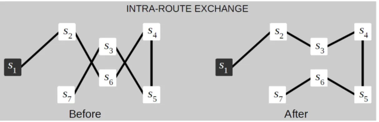
Intra-route exchange

(41)

A stop may switch its position with another stop, both in the same route. This is illustrated in Figure 5.2. That is, at each route r ∈ R two non-mandatory stop si and sj , not between the same pair of mandatory stops, with the shortest distance between them are picked. If a better feasible solution is obtained by switching these stops then removal and relocation occurs. This can be done many times, while the feasible solution is improve.

Inter-route relocation

Figure 5.3: Inter-route relocation.

Inter-Route Relocation: A stop may be moved to another route. This is illustrated in Figure 5.3. That is, for each route r ∈ R the non-mandatory stop s with the longest dis-tance from its predecessor and successor is picked. If a better feasible solution is obtained by moving this stop to another route then removal and relocation occurs. The new route and place should be the one with the shortest distance from s to the new predecessor and successor stops. This can be done while the feasible solution is improved.

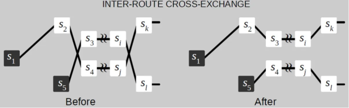
Inter-route cross-exchange

Figure 5.4: Inter-route cross-exchange.

Two sets of consecutive stops of two different routes may be switched. This is illus-trated in Figure 5.4. That is, the two stops si and sj with the shortest distance between

(42)

them, and belonging to different routes, are initially picked. Stop si will be part of set A while stop sj will be part of set B. Then, sets A and B are extended, by including a consecutive nearby stop, while a better feasible solution is obtained if sets were switched. The consecutive nearby stop should be the one that minimizes the total distance from all stops of one set to all stops of the other set. This can be done while the feasible solution is improved.

(43)

C H A P T E R

6

Result analysis

6.1 Result analysis

In this section the results obtained by the proposed heuristic algorithm are analysed. Since the instance sets available in the literature to evaluate vehicle routing problems can not be directly applied to our VRwBP problem, the instance sets commonly used to evaluate multi-depot vehicle routing problem (MDVRP) heuristics, described in [41], have been adopted while making some assumptions. Both instance sets and best known results for the MDVRP are available in [42].

6.1.1 Assumptions

The MDVRP instances include information about the number of depots available, maxi-mum number of vehicles available per depot, and nodes/stops to be visited. For each stop, its coordinates, service time and demand are given. The P instances have 0 of service time and vehicles do not return to the depot while PR instances have non-zero service times and vehicles return to the depot. For the VRwBP problem under analysis the following assumptions must be applied for each instance:

• Stops requiring backup, B, will be the ones having more demand. Different B set sizes will be tested.

• To define the total number of routes in R, the solutions provided by the best known heuristic results were used. In such solutions, if m vehicles leave a specific depot then m empty routes starting at that depot will be included in R. This choice is based on the fact that best known solutions provide good upper bounds on the num-ber of routes required to cover all stops. Therefore, it is not necessary to consider all vehicles available per depot (info provided by MDVRP instances).

• Considering a specific depot siand the m routes starting at si, determined as stated

(44)

6.1 Result analysis

farther away from si, one for each route. That is, each route has two mandatory

stops, the depot and one of the m stops.

• Due to the way mandatory stops have been defined, a reasonable time window for a mandatory stop s at route r will be:

∆(s0, s) = duration(r) − P

sk∈Sservice(sk)

|R|

where duration(r) is the total duration of route r, provided by the best known results, and service(sk) is the service time at stop sk. That is, the average total

service time per route is removed from the total duration of the route, since service time is not relevant for our VRwBP problem. This result must be divided by 2 for PR instances because the total duration of routes include returning to the depot, and this must not be considered when defining the time windows of mandatory stops. • The threshold of a critical node sj, denoted by Tsj, will be a percentage of sj’s

route duration, i.e, route of the best known results where sj is inserted. Thus,

Tsj = p × duration(r), sj ∈ r, 0 < p ≤ 1. Different percentage values will be

tested.

The following analysis includes only the results for the 52 node instances available in [42]. Please note that the planning under discussion in this article does not take route schedules into consideration. Therefore, besides the just mentioned instance related as-sumptions, it is also assumed that route schedule assignment is done, after route planning, in a way that vehicles finish their route in time to provide backup to their associated criti-cal nodes.

6.1.2 Backup provisioning and pos-optimal impact analysis

In this section we analyse the impact of planning vehicle routes with backup provisioning. Since the heuristic will run for many instances, having different service times, demands, etc, there might be different performances for different instances. For this reason, to analyse the impact of backup provisioning (BP) the following gap is analysed:

GapBP_i = Distance BP i − DistanceN oBPi DistanceN oBP i (6.1) where DistanceBP_i is the distance value obtained when backup is provided and DistanceN oBP_i is the distance value obtained if no backup is provided, considering a specific instance i. Results shown in the following plots include the average of these gaps, over all analysed instances.

(45)

6.1 Result analysis

Figure 6.1: Increase on distance values, obtained by the heuristic, when backup is provided.

Regarding the effectiveness of pos-optimal (PO) procedures, and also due to the fact that there will be many instances, the following gap is analysed:

GapP O_i = Distance N oP O i − DistanceP Oi DistanceN oP O i (6.2) where DistanceN oP O

i is the distance value obtained when no pos-optimal procedures are

used and DistanceP O

i is the distance value obtained after applying pos-optimal

proce-dures, considering a specific instance i. Results plotted in the following figures include the average of these gaps over all analysed instances.

Figure 6.1 shows the increase on distance values, obtained by the heuristic, when backup is provided to critical nodes. Results show that the increase on the distance values gets higher as the number of critical stations increases, as expected, reaching_{v 15% for} four critical nodes, while for a single node it reachedv 2.5%. However, when the thresh-old gets more loose the gap between backup and no backup solutions reduces, whatever the number of critical nodes, as less route extensions are required for backup provisioning. Please note that extra route duration in case of backup provisioning also means serving more stops meaning that this is not necessarily a disadvantage. In fact stop weights can be used at the backup inclusion step in order to extend routes using stops with more visiting needs. Therefore, the right balance between threshold, influencing route extension, and number of routes should be carefully planned in order to reduce the operational costs related with the number of route schedules, and vehicles, while providing high quality

(46)

6.1 Result analysis

Figure 6.2: Decrease on distance values, obtained by the heuristic, when pos-optimal procedures are applied. Backup is being provided.

service and customer satisfaction.

Regarding the improvement on distance values, when using pos-optimal procedures, Figure 6.2 shows the decrease on the distance values obtained when pos-optimal proce-dures are applied, assuming that backup is being provided to critical stops. As it can be observed, pos-optimal procedures are very effective reducing the overall route lengths in approximately 30%. When no backup is provided the distance value reduction, which is independent of the number of critical stops and threshold, was also 30%.

It is also possible to conclude from Figure 6.2 that the optimal threshold value is around 10%. More tight thresholds result into lower pos-optimal procedure improve-ments. For threshold values higher than 10% the decrease of pos-optimal procedure im-provements is low. Since tight thresholds lead to longer route extensions, while loose thresholds result into few or no route extensions, we can state that the insertion of just a few stations for route extension is enough to reach the best improvements. No station in-sertion means less flexibility when making exchange/relocation, while the inin-sertion of too many stations result into longer routes and exchange/relocation is not able to compensate such increase.

Figure 6.3 shows the average of the ratios between the time it takes for a vehicle finishing its route somewhere in the neighbourhood, and providing backup, to come to the critical station and the time it takes for a new vehicle to come from the depot, so that

(47)

6.1 Result analysis

Figure 6.3: Backup provisioning vs vehicle from depot time radio.

extra clients are accommodated. When looking into this plot we can observe that backup provisioning times are always lower than the times associated with the routes that would be traversed if a new vehicle comes from the source. Note also that, in this last case, a new schedule, vehicle and driver needs to be introduced. In case of backup provisioning there is no need for a new schedule, extra vehicle and driver.

When observing this last plot we can state that higher threshold values result into a more pronounced increase of ratio values because not only backup takes more time to arrive but also routes become shorter. It is also possible to observe that since the threshold for a critical node is a percentage of the route duration, where the critical node is inserted, more critical nodes do not necessarily lead to a smoothing of the average values plotted, at least for lower threshold values. This would be the case if similar absolute thresholds were used for all critical nodes.

6.1.3 Overall perception

From the previous analysis done, the overall perception is that planning routes with backup provisioning can allow fast response to overload while reducing costs since:

• Backup provisioning allows fast response to overload and reduces waiting times for customers;

(48)

6.1 Result analysis more needs;

• Backup provisioning avoids more schedules/vehicles/drivers, reducing costs; • The extra traversal by a vehicle providing backup is only done in case of need,

namely when sensors detect overcrowding in a critical stop. This is flexible and cost effective solution for transportation network enhancement.

(49)

C H A P T E R

7

Conclusions and future work

In this thesis a vehicle routing with backup provisioning approach is proposed for sustain-able urban mobility with efficient use of resources. Besides mathematically formalizing the problem, a heuristic is also proposed that allows good solutions to be obtained faster. This heuristic incorporates pos-optimal procedures that significantly improve the quality of the initial solutions obtained by the heuristic. Results show that vehicle routing with backup provisioning can be a very flexible and cost effective solution for transportation network enhancement, while improving the quality of experience for customers.

The overall perception from these results is that planning routes with backup provi-sioning can allow fast response to overload while reducing costs since:

• Extension of routes to incorporate a backup can be done while serving stops with more needs;

• Backup provisioning from a vehicle in the neighbourhood allows fast response to overload and reduces waiting times for customers;

• Backup provisioning from a vehicle in the neighbourhood avoids having more schedules, and therefore vehicles and drivers, reducing costs. Also, fleet vehicles can be smaller since an empty vehicle in the neighbourhood will arrive in case of overload;

• The extra traversal by a vehicle providing backup is only done in case of need, namely when sensors detect overcrowding in a critical stop.

From such discussion we do believe that transportation network enhancement using sensors can bring real benefits as smart vehicle routing decisions, like reacting to overload, can be done.

For future work we expect to:

• Add features to monitoring tool: Show the new routes incorporating backup provi-sioning, time comparison with previous routes and allow companies to interchange data. Also, the possibility of assigning schedules and drivers can be added.

(50)

Conclusions and future work

• Heuristic: Improve the insertion of the remaining stops (last step before backup inclusion).

• Higher data sets: Test higher data sets and analyse results. Different data sets may produce different optimal threshold values.

• Real tests: On the field implementation to see data collecting and real optimization of routes, in a big fleet scenario.

Monitoring of urban transportation networks using wireless sensor networks

UNIVERSIDADE DO ALGARVE