Longitudinal modeling in sports: Young swimmers’ performance and biomechanics proﬁle

(1)

Longitudinal modeling in sports: Young

swimmers’ performance and biomechanics profile

Jorge E. Morais

a,e

, Mário C. Marques

b,e

, Daniel A. Marinho

b,e

,

António J. Silva

c,e

_{, Tiago M. Barbosa}

d,e,⇑

a_{Department of Sport Sciences, Polytechnic Institute of Bragança, Bragança, Portugal}

b_{Department of Sport Sciences, University of Beira Interior, Covilhã, Portugal}

c_{Department of Sport Sciences, Exercise and Health, University of Trás-os-Montes and Alto Douro, Vila Real, Portugal}

d_{National Institute of Education, Nanyang Technological University, Singapore, Singapore}

e_{Research Centre in Sports, Health and Human Development, Vila Real, Portugal}

a r t i c l e

i n f o

Article history:

PsycINFO classification: 3720

Keywords: Modeling Kinematics Hydrodynamics Season adaptations Contribution

a b s t r a c t

New theories about dynamical systems highlight the multi-factorial interplay between determinant factors to achieve higher sports performances, including in swimming. Longitudinal research does provide useful information on the sportsmen’s changes and how training help him to excel. These questions may be addressed in one single procedure such as latent growth modeling. The aim of the study was to model a latent growth curve of young swimmers’ performance and biomechanics over a season. Fourteen boys (12.33 ± 0.65 years-old) and 16 girls (11.15 ± 0.55 years-old) were evaluated. Performance, stroke frequency, speed fluctuation, arm’s propelling efficiency, active drag, active drag coefficient and power to overcome drag were collected in four different moments of the season. Latent growth curve modeling was computed to under-stand the longitudinal variation of performance (endogenous vari-ables) over the season according to the biomechanics (exogenous variables). Latent growth curve modeling showed a high inter-and intra-subject variability in the performance growth. Gender had a significant effect at the baseline and during the performance growth. In each evaluation moment, different variables had a meaningful effect on performance (M1: Da,b=0.62; M2:Da,

b=0.53; M3:gp,b= 0.59; M4: SF,b=0.57; allP< .001). The

models’ goodness-of-fit was 1.406v2_/df₆_3.74

⇑Corresponding author at: Physical Education & Sports Science Academic Group, National Institute of Education, Nanyang Technological University, NIE5-03-31, 1 Nanyang Walk, Singapore 637616, Singapore. Tel.: +65 6219 6213; fax: +65 6896 9260.

E-mail address:tiago.barbosa@nie.edu.sg(T.M. Barbosa).

Contents lists available atScienceDirect

Human Movement Science

(2)

able). Latent modeling is a comprehensive way to gather insight about young swimmers’ performance over time. Different variables were the main responsible for the performance improvement. A gender gap, intra- and inter-subject variability was verified.

1. Introduction

Talent identification, development, and follow-up are some of the major challenges that sports researchers and practitioners still face nowadays. Swimming performance is characterized by the multi-dimensional interplay of different scientific fields, where a highly complex interaction between several variables exists (Barbosa et al., 2010). Cross-sectional studies reported relationships between young swimmers’ performance, Energetics (Toubekis, Vasilaki, Douda, Gourgoulis, & Tokmakidis, 2011), Biomechanics (Morais et al., 2012) and Motor Control (Silva et al., 2013). Nevertheless, from among all these scientific fields, Biomechanics plays a major role by explaining 50–60% of the perfor-mance of young swimmers (Morais et al., 2012). Probably the partial contribution of each key factor to performance may change across time, for example, over a season. However, until now no longitudinal research has been conducted about it in sports performance. Moreover, longitudinal research should help in gathering insight into: (i) how biomechanical variables interplay and affect performance; (ii) the dynamical changes that happen at these early ages; (iii) the partial contribution of each determi-nant factor over time.

For a long time sports research was based on the assumption that intra- and inter-subject var-iability should be minimized. Nowadays, dynamic systems theory and non-linear approaches sug-gest that variability should not be considered as a random error (Bideault, Herault, & Seifert, 2013). Evidence has been gathered lately about this topic in adult/elite swimmers (Costa et al., 2013; Komar, Sanders, Chollet, & Seifert, 2014) even though definitive answers are needed. Besides this, little or almost nothing is known about it in young swimmers. Interestingly young sportsmen, including swimmers, are supposed to be among the ones with a higher variability due to their allegedly low expertise level. It seems that athletes with lower (such as young swimmers) and very high expertise (including elite swimmers) levels are the ones with the highest variability (Seifert et al., 2011).

Until now, classical research designs and data analysis procedures (e.g., analysis of variance and regression models) selected on regular basis in sports performance were not helpful in gathering insight about such highly dynamic and complex relationships. Latent growth curve modeling is a structural equation modeling technique for longitudinal dataset. It is characterized by estimating intra- and inter-subject growth trajectories, enabling researchers to predict future development (Wu, Taylor, & West, 2009). Structural equation modeling also allows the quantification of how much an exogenous variable contributes to an endogenous variable (Morais et al., 2012). Hence, its potential to explain complex and dynamic changes as reported earlier should be explored. This longitudinal data analysis procedure is reported on regular basis in Social Sciences such as Psychol-ogy (Biesanz, West, & Kwok, 2003; Castellanos-Ryan, Parent, Vitaro, Tremblay, & Séquin, 2013). In Sport Sciences a couple of papers can be found on physical fitness and health (Maia et al., 2003; Park & Schutz, 2005) but it was never attempted in sports performance as much as we are aware of.

Therefore, the aim of this study was to model a latent growth curve of young swimmers’ per-formance and biomechanics over a season. It was hypothesized that latent growth curve modeling would explain performance improvement. Different exogenous variables would have a higher contribution on the performance enhancement throughout the season with a significant gender effect.

(3)

2. Methods

2.1. Subjects

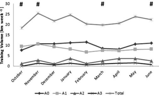
Thirty young swimmers, including 14 boys: 12.33 ± 0.65-y, 284.85 ± 67.48 FINA (Fédération Inter-nationale de Natation) points at the short-course meter (i.e., 25-m length swimming pool) 100-m free-style; and 16 girls: 11.15 ± 0.55-y, 322.56 ± 45.18 FINA points at the short-course meter 100-m freestyle were recruited. All swimmers were in Tanner stages 1–2 by self-report at baseline (Tanner, 1962). The sample included age-group national record holders and champions. The swim-mers were part of a national talent ID scheme. At the beginning of the research the swimswim-mers had 3.40 ± 0.56 years of training experience.Fig. 1reports the external training load over the season. Coa-ches, parents, and/or guardians consented and the athletes assented their participation on this study. All procedures were in accordance to the Helsinki Declaration regarding Human Research. The Univer-sity of Trás-os-Montes and Alto Douro Ethic Committee also approved the study design (ethic review: UTAD-2011-219).

2.2. Study design

The research design (Fig. 2) included repeated measures of kinematic and hydrodynamic variables in four different moments over one season (i.e., longitudinal research). Testing sessions happened immediately before the beginning of the season (baseline-M1), 4 weeks later (first competition-M2), in the middle of the season (24th week-M3) and at the end of the season (38th week-M4). Data collection procedures were carried out in the same conditions at all times (e.g., the same swimming pool, lane, time of day).

2.3. Theoretical model

Theoretical model (Fig. 3) was designed to include kinematic, hydrodynamic, and performance, controlling the gender effect. Stroke frequency (SF), intra-cyclic speed fluctuation (dv) and propelling efficiency (

g

p) were selected as kinematic outcomes. As for hydrodynamics, active drag (Da),

coefficient of active drag (CDa) and power to overcome drag (Pd) were selected. Literature reports that

(4)

kinematics and hydrodynamics determine young swimmers’ performance (Morais et al., 2012). Stroke frequency, speed fluctuation, and arm’s propelling efficiency (i.e., kinematics), active drag, coefficient of active drag, and power to overcome drag (i.e., hydrodynamics) are some of the variables that have a strong relationship with young swimmers’ performance and therefore were selected on regular basis in swimming research (Marinho et al., 2010; Morais et al., 2012; Silva et al., 2013).

Swimming performance was chosen as the main outcome (endogenous variable; i.e., dependent variable being predicted), because the primary goal of coaches and swimmers is to enhance the per-formance. Kinematic and hydrodynamic variables are the exogenous variables (i.e., independent vari-ables that predict the main outcome). The interpretation of this kind of approach is based on: (i) the variables included (inserted inside squares); (ii) the paths (i.e., arrows; an arrow between two variables means that one variable determines the other); (iii) beta values (i.e., these suggest the

Fig. 2.Study design scheme. M – moment; Wk – week; # – week’s number.

Fig. 3.Theoretical model. VAR (1, 2, 3 and 4) – exogenous variable in M1, M2, M3 and M4, respectively; PERF (1, 2, 3 and 4) – performance in M1, M2, M3 and M4, respectively; ICEPT – intercept effect; SLOPE – slope effect; Gender – gender effect;bxi,yi– beta value for regression model between exogenous (xi) and endogenous (yi) variables;exi– disturbance term for a given variable;xi?yi– variableyidepends from variablexi.

(5)

contribution of one variable to the other; when the origin variable increases by one unit the destina-tion variable increases by the amount of the beta value); (iv) residual errors and/or determinadestina-tion coefficient (represents the variable predictive error or the variable predictive value, respectively, in the linked ellipse), and (v) the latent variables (inserted in ellipses) are the no-observed (i.e., the slope analyzes the endogenous variable growth and variability; the intercept analyzes the variability in the baseline).

It was possible to extract the following details from the model: (i) the direct effect (i.e., contribu-tion) of an exogenous variable to the endogenous one (i.e., performance) in each evaluation moment; (ii) the longitudinal growth of the endogenous variable; and (iii) the gender influence at the baseline values (intercept) and also in the endogenous variable growth (i.e., slope).

2.4. Performance data collection

The official short course 100-m freestyle race was chosen as performance variable. The time gap between each the race and data collection took no longer than 15-days.

2.5. Kinematics data collection

Swimmers were instructed to perform three maximal trials of 25-m at front-crawl with push-off start. Between each trial they had a 30-min rest to ensure full recovery. For further analysis the aver-age value of the three trials was calculated (ICC = 0.96).

Kinematic data was collected with a mechanical technique (Swim speedo-meter, Swimsportec, Hil-desheim, Germany). A 12-bit resolution acquisition card (USB-6008, National Instruments, Austin, Texas, USA) was used to transfer data (f= 50 Hz) to a customized software (LabVIEWÒ

interface, v.2009) (Barbosa et al., 2010). Data were exported to a signal processing software (AcqKnowledge v.3.9.0, Biopac Systems, Santa Barbara, USA) and filtered with a 5 Hz cut-off low-pass 4th order But-terworth filter. Speed fluctuation was computed as (Barbosa et al., 2010):

dv¼

ffiffiffiffiffiffiffiffiffiffiffiffiffiffiffiffiffiffiffiffiffiffiffiffiffiffiffiffiffiffiffiffiffiffiffi P

ið

v

i

v

_Þ2Fi₌n q

P i

v

iFi=n

ð1Þ

where dv is the speed fluctuation,

v

is the mean velocity,

v

_iis the instant velocity,F_iis the absolute

frequency andnis the number of observations per stroke cycle. Two expert evaluators measured the SF with a stroke counter (base 3) and then converted to SI units (ICC = 0.98). The

g

pwas estimated

as (Zamparo, Pendergast, Mollendorf, Termin, & Minetti, 2005):

g

p¼

v

0:9 2

p

SFl

2

p

100 ð2Þ

where

g

pis the arm’s propelling efficiency,

v

is the velocity, SF is the stroke frequency andlis the

dis-tance between shoulder and tip of the 3rd finger during the insweep.

2.6. Hydrodynamics data collection

The Velocity Perturbation Method was selected to assess the hydrodynamic variables (Kolmogorov & Duplisheva, 1992). Swimmers performed two extra maximal trials of 25-m at front crawl with push-off start (one trial with and the other without carrying on the perturbation device). Swimming velocity was assessed between the 11th and 24th m from the starting wall (Marinho et al., 2010). The time spent to cover this distance was measured with a manual stopwatch (Golfinho Sports MC 815, Aveiro, Portugal) by two expert evaluators (ICC = 0.97). The evaluators followed the swimmer to a have a good line of sight when the swimmer passed the two distance marks. TheDawas estimated as (Kolmogorov

& Duplisheva, 1992):

Da¼Db

v

b

v

2

v

3

v

3 b

(6)

whereDais the swimmers’ active drag at maximal velocity,Dbis the resistance of the perturbation

buoy provided by the,

v

_band

v

are the swimming velocities with and without the perturbation device.

TheCDawas calculated as (Kolmogorov & Duplisheva, 1992):

CDa¼ 2Da

q

S

v

2 ð4Þ

whereCDais the active drag coefficient,

q

is the water density (assumed to be 1000 kg m3),

v

is the

velocity andSis the swimmers’ projected frontal surface area. ThePdwas obtained from (Kolmogorov

& Duplisheva, 1992):

Pd¼D

v

_ð5_Þ

wherePdis the power to overcome drag,Dis the drag and

v

is the velocity.

2.7. Statistical procedures

The normality and homoscedasticity assumptions were analyzed with the Shapiro–Wilk and the Levene tests, respectively. Descriptive statistics included the calculation of the mean, median, mini-mum, maximum and one standard deviation.

Latent growth curve modeling was used to compute the longitudinal variation of the swimmers’ performance over the season. This technique is characterized by estimating intra-individual (repre-sented by the growth parameters; i.e., intercept and slope for growth) in the inter-individual (differ-ences between subjects) growth trajectories (Wu et al., 2009). The intercept and slope are latent variables, which means that they are not directly observed but rather inferred. The intercept deter-mines where the participants’ baseline is and how they differ in that specific moment, showing the inter-individual differences between the participants at the baseline, corresponding to M1 in this model). The slope is the average rate of growth, related to the variation throughout a time-frame. It shows the hypothetical differences between the observed moments, and if an inter-individual vari-ability exists or not.

The effect between exogenous (SF, dv,

g

p,Da,CDa, andPd) and endogenous (performance) variables

was also considered. Endogenous variable is the one being predicted and the growth rate analyzed. Exogenous variables are the ones with a direct effect on performance in each evaluation moment. Path-flow analysis model was used to estimate the linear regression standardized coefficients between exogenous and endogenous variables. Standardized regression coefficients (b) were selected, and the significance of each one assessed with Student’sttest (P6.05).

The models’ goodness-of-fit were measured with the ratio Chi-square/degrees of freedom (

v

2_/df)

(Wheaton, 1987). As a rule of thumb if: 5 <

v

2_{/df the model has a poor adjustment; 2 <}

_v

2_/df

65

rea-sonable adjustment; 1 <

v

2_/df₆_{2 good adjustment;}

_v

2_/df

1 very good adjustment.

3. Results

Performance improved between the first (M1, 72.05 ± 5.33 s) and last (M4, 66.13 ± 5.16 s) evalua-tion moments.DaandPdshowed the highest variations across the season (Table 1). Some selected

variables (

g

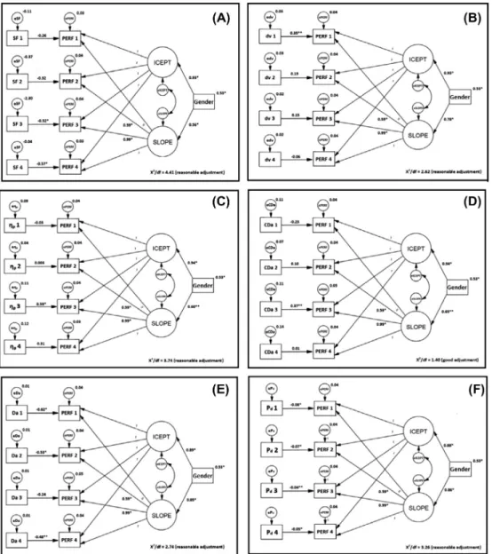
p,Da,CDaandPd) increased in a non-linear fashion way.

In M2 and M3, performance achieved 59% (P< .001) and 99% (P< .001) of the last evaluation (M4) (Fig. 4). The slope variance was significant for all models, suggesting a heterogeneous growth rate of the performance and hence an inter-subject variability for the pooled sample (i.e., boys plus girls). The dv model was the one presenting the highest slope (b= 6.56;P= .003). The intercept variance was sig-nificant for all models computed, suggesting an inter-subject variability at the baseline for the pooled sample and

g

pshowed the highest intercept (b= 28.15;P< .001). Overall it seems that each

partici-pant had its own and unique growth rate suggesting a high inter-subject variability.

Gender had a significant effect on the performance growth with significant paths to intercept and slope for all models (Fig. 4). Both

g

pandCDamodels presented the highest significant paths (b= 0.94;

(7)

P< .001). Data showed that boys presented better performances than girls. ThePdmodel had the

high-est significant path (b= 0.86;P< .001).

All selected variables presented a significant direct effect on performance at least in one evaluation moment (Fig. 4). In M1 theDapresented the highest direct effect on performance (b=0.62;P< .001;

by each 1N increase, performance improved 0.62 s). In M2 was once again theDa(b=0.53;P< .001),

in M3 the

g

p(b= 0.59;P< .001) and in M4 the SF (b=0.57;P< .001). Hence, swimmers relied on

dif-ferent exogenous variables to enhance performance in difdif-ferent moments of the season.

(8)

Table 1

Descriptive statistics for selected kinematic and hydrodynamic variables in each evaluation moment.

PERF [s] SF [Hz] dv [dimensionless] gp[%]

M1 M2 M3 M4 M1 M2 M3 M4 M1 M2 M3 M4 M1 M2 M3 M4

Mean 72.05 68.91 66.44 66.13 0.85 0.84 0.86 0.86 0.09 0.09 0.08 0.08 30.21 30.38 33.13 31.03

1 SD 5.33 5.43 5.33 5.16 0.09 0.08 0.10 0.08 0.02 0.03 0.02 0.01 2.94 2.94 4.55 5.13

Median 72.02 69.32 67.43 66.66 0.83 0.83 0.83 0.83 0.09 0.09 0.08 0.08 30.47 30.78 32.12 30.73

Minimum 60.30 57.03 58.01 57.36 0.67 0.70 0.72 0.73 0.06 0.06 0.06 0.05 25.16 24.24 26.00 24.12

Maximum 81.00 79.12 76.85 76.06 1.05 0.99 1.07 1.03 0.16 0.17 0.14 0.10 35.80 35.06 44.99 53.06

Da[N] CDa[dimensionless] Pd[W]

M1 M2 M3 M4 M1 M2 M3 M4 M1 M2 M3 M4

Mean 45.84 71.01 83.25 75.62 0.40 0.49 0.58 0.50 68.65 99.04 116.93 109.62

1 SD 27.76 33.70 37.30 36.96 0.22 0.17 0.26 0.22 47.12 49.90 53.83 57.08

Median 34.29 58.36 70.85 77.05 0.34 0.48 0.51 0.46 49.22 81.72 97.36 107.25

Minimum 22.20 26.64 22.20 20.66 0.16 0.22 0.18 0.18 31.34 36.55 30.44 24.00

Maximum 139.53 167.33 172.93 189.52 1.41 0.89 1.28 1.32 241.54 229.86 244.27 295.41

Mi – evaluation moment; PERF – performance; SF – stroke frequency; dv – speed fluctuation;gp– arm’s propelling efficiency;Da– active drag;CDa–active drag coefficient;Pd– power to overcome drag.

118

J.E.

Morais

et

al.

/Human

Movement

Science

37

(2014)

(9)

The models’ goodness-of-fit ranged between 1.406

v

2_/df₆_{3.74 (i.e., good-reasonable). The}_C Da

model showed highest goodness-of-fit (

v

2_{/df = 1.40; good adjustment) and the SF the lowest one}

(

v

2_{/df = 4.41; reasonable adjustment).}

4. Discussion

The main aim of this study was to model a latent growth curve of swimming performance and its relationship with biomechanics over time to gather insight about the partial contribution of each fac-tor and the gender effect. In the first two moments, hydrodynamics was the major contribufac-tor to per-formance and in the last two, kinematics. The model was also able to detect a gender gap and a high intra- and inter-subject variability. Therefore, over a season, different determinant factors had a main influence on the performance enhancement for both boys and girls. Besides that, each one of them selected a unique strategy to enhance performance.

Cross-sectional studies showed that young swimmers’ performance is highly influenced by kine-matics and hydrodynamics (Morais et al., 2012). However, longitudinal follow-up studies that included these variables neglected the inter- and intra-subject changes (Lätt et al., 2009). At least for adult swimming it was pointed out that intra-subject changes are not residual variance and it should not be disregarded in the overall analysis (Connaboy, Coleman, Moir, & Sanders, 2010; Costa et al., 2013). The same idea was shared earlier by others for motor control (Komar et al., 2014) and kinematics changes (Figueiredo, Seifert, Vilas-Boas, & Fernandes, 2012; Seifert, Barbosa, & Kjendlie, 2010; Seifert, Leblanc, Chollet, & Delignières, 2010). Latent growth curve modeling is able to estimate intra- and inter-subject variability. Variance analysis showed significant differences between swim-mers at the baseline and during the performance growth. Residual variances tend to be neglected by other data analysis techniques (e.g., analysis of variance and multi-linear regressions). At least clas-sical techniques are less sensitive to such residual variances. However, those variances are of major interest in latent growth curve modeling (Voelkle, 2007). A main finding of this research was that young swimmers presented a high intra- and inter-subject variability suggesting that each one has a very unique strategy to excel.

Latent growth curve modeling provides the amount of performance that is achieved in intermedi-ate moments. Between M1 and M2 performance reached 59% of its final value in M4. Between com-petitive seasons, young swimmers have a break period impairing their energetics and kinematics (Moreira et al., 2014). The improvement between M1 and M2 might be related with the first meso-cycle that is characterized by a fairly high volume after the summer break (Fig. 1). Afterwards, perfor-mance improved 39% (between M2 and M3) and 1% (between M3 and M4). Hence, as the major competition of the season is approaching, improvements are less sharp and meaningful. Similar trend is reported for adult/elite swimmers. Building-up for the major competition, adult swimmers are get-ting closer from their reserve upper-limits, and it is more challenging for any further improvement (Costa et al., 2013).

A gender gap was also identified at the baseline and during the performance growth. There is a very solid body of knowledge about the gender differences for peri- and post-pubertal athletes (Seifert, Barbosa et al., 2010; Seifert, Leblanc et al., 2010). Literature reports that boys have a higher dv,Da,

and SF than girls (Barbosa et al., 2010). Therefore longitudinal structural equation modeling was suc-cessful in identifying the well-known gender gap. In this sense, the technique used is also sensitive enough whenever pooled data (both genders) is computed.

Swimming is characterized by the multi-dimensional interplay of different variables that will influ-ence the performance. One might claim that the partial contribution of each exogenous variable to the endogenous one will change over time. That is, the partial contribution of each variable will not be constant over time. However, until now as much as we are aware no paper reported or quantified such phenomenon. Structural equation modeling is very sensitive to such changes and can be used to learn about it. In M1 and M2,Dawas the main performance determinant. Between M1 and M2 periodization

(10)

performance (Havriluk, 2006). Da is strongly related to swimming velocity (Eq. (3)). Hence, the

increase in speed and therefore in performance lead to a higherDa.CDahad a minor influence on

per-formance growth. So, it can be speculated that the perper-formance enhancement during this time frame might be more related to energetic build-up and less to technique enhancement.

In M3,

g

phad the highest direct effect on the performance. Between M2 and M3 periodization was

characterized by a decrease in total volume (Fig. 1). These meso-cycles were more focused on techni-cal parameters (enhancing stroke mechanics). This explains why on average the swimmers achieved the highest

g

pin M3. Since long there has been a discussion whether young swimmers training should

rely more on energetics or efficiency. Cross-sectional confirmatory models suggested that 50–60% of performance in these age-groups is related to biomechanics and technique enhancement (Morais et al., 2012). In M4, SF was the variable presenting the highest direct effect on performance. Between M3 and M4 periodization included an increase in the aerobic power and aerobic capacity sets (Fig. 1). This was coupled with a slight increase of the dry-land training sessions that included strength power routines. For adolescent sprint swimmers, an association was found between high muscular strength parameters and an increase in SF (Girould, Maurin, Dugué, Chatard, & Millet, 2007). At least in adult swimmers aerobic power paces are related to customize SF-stroke length relationships (McLean, Palmer, Ice, Truijens, & Smith, 2010; Wakayoshi, D’Acquisito, Cappert, & Troup, 1995). Therefore, to swim at aerobic power sets a fairly constant and high stroke length with a high SF is needed. To be able to optimize this SF-stroke length relationship dry-land power training is a must.

It was attempted in one of the earliest models to include anthropometrics variables to control the potential confounding factor of the maturation and growth. However, after running the model, we failed to obtain significant results and a reasonable adjustment. Because we track down and follow-up subjects in Tanner 1–2, one might consider that most of them are yet pre-pubescent and therefore one single year is not enough to verify significant changes in biological maturation. With this we are not suggesting that they are not in a process of biological development but only that because they did not reach any spur, it is more challenging to have anthropometrics as a determinant factor. However, later one, that is, swimmers in the following Tanner stages this is more obvious (Falk, Bronshtein, Zigel, Constantini, & Eliakim, 2004; Jurimae et al., 2007). Overall, in M1 and M2 hydrodynamics (i.e., Da) was the major contributor to performance while in M3 and M4 was the kinematics (

g

p

and SF, respectively). Therefore, the main determinant at a given moment is related to the periodiza-tion model designed. It is possible to design models that are more based on energetics (M1 and M2) or technique (M3 and M4). A model that relies more on energetics allows a very quick and sharp improvement, but on the other hand the efficiency is compromised and increases the odds of an early burn-out. A model that is based on the technique is more time-consuming and performance enhance-ment might take some time to happen. However, a proper technique will be needed for further improvement reaching adulthood, when most of the periodization is energetically oriented (e.g., Schnitzler, Seifert, Chollet, & Toussaint, 2014). Besides, it is at these early ages that the motor learning mechanisms of any skill is more effective. Considering the pros and cons of each approach, an age-group coach should consider to compromise both (energetics build-up and technique enhancement) but putting more focus on the technique and efficiency if the athlete’s career is to be seen in the long-run. Hence, it seems that many of the changes in performance can be attributed to the type of training that swimmers were undergoing at the time of each data collection. This could be useful for coaches as it shows that technical parameters are the most determinant ones in the young swim-mers’ performance improvement. They can apply these technical drills according to their macro-cycles, avoiding the athletes to burn out with high amounts of training workloads, especially close to the main events.

5. Conclusion

(11)

strategy is used by each swimmer to excel. Overall it seems that young swimmers coaches’ should put the focus on the hydrodynamic profile and also on the stroke mechanics (i.e., technical ability) to enhance the performance, notably sprinters. Moreover the performance main determinants are also related to the training periodization.

Conflict of interest

The authors have no professional relationships to disclose with companies or manufacturers who will benefit from the results of the present study.

Acknowledgments

Jorge E. Morais gratefully acknowledges the Ph.D. scholarship granted by the Portuguese Science and Technology Foundation (FCT) (SFRH/BD/76287/2011). The authors wish to thanks Pedro Forte and Marc Moreira for their useful help during data collection.

References

Barbosa, T. M., Bragada, J. A., Reis, V. M., Marinho, D. A., Carvalho, C., & Silva, A. J. (2010). Energetics and biomechanics as determining factors of swimming performance: Updating the state of the art.Journal of Science and Medicine in Sport, 13, 262–269.

Bideault, G., Herault, R., & Seifert, L. (2013). Data modelling reveals inter-individual variability of front crawl swimming.Journal of Science and Medicine in Sport, 16, 281–285.

Biesanz, J. C., West, S. G., & Kwok, O. M. (2003). Personality over time: Methodological approaches to the study of short-term and long-term development and change.Journal of Personality, 71, 905–941.

Castellanos-Ryan, N., Parent, S., Vitaro, F., Tremblay, R. E., & Séquin, J. R. (2013). Pubertal development, personality, and substance use: A 10 year longitudinal study from childhood to adolescence.Journal of Abnormal Psychology, 122, 782–796. Connaboy, C., Coleman, S., Moir, G., & Sanders, R. (2010). Measures of reliability in the kinematics of maximal undulatory

underwater swimming.Medicine and Science in Sports and Exercise, 42, 762–770.

Costa, M. J., Bragada, J. A., Mejias, J. E., Louro, H., Marinho, D. A., Silva, A. J., et al (2013). Effects of swim training on energetics and performance.International Journal of Sports Medicine, 34, 507–513.

Falk, B., Bronshtein, Z., Zigel, L., Constantini, N., & Eliakim, A. (2004). Higher tibial quantitative ultrasound in young female swimmers.British Journal of Sports Medicine, 38, 461–465.

Figueiredo, P., Seifert, L., Vilas-Boas, J. P., & Fernandes, R. J. (2012). Individual profiles of spatio-temporal coordination in high intensity swimming.Human Movement Science, 31, 1200–1212.

Girould, S., Maurin, D., Dugué, B., Chatard, J. C., & Millet, G. (2007). Effects of dry-land vs. resisted- and assisted-sprint exercises on swimming sprint performances.Journal of Strength and Conditioning Research, 21, 599–605.

Havriluk, R. (2006). Magnitude of the effect of an instructional intervention on swimming technique and performance. In J. P. Vilas-Boas, F. Alves, & A. Marques (Eds.),X International symposium of biomechanics and medicine in swimming(pp. 218–220). Porto: Portuguese Journal of Sport Sciences.

Jurimae, J., Haljaste, K., Cicchella, A., Latt, E., Purge, P., Leppik, A., et al (2007). Analysis of swimming performance from physical, physiological, and biomechanical parameters in young swimmers.Pediatric Exercise Science, 19, 70–81.

Kolmogorov, S., & Duplisheva, O. (1992). Active drag, useful mechanical power output and hydrodynamic force in different swimming strokes at maximal velocity.Journal of Biomechanics, 25, 311–318.

Komar, J., Sanders, R. H., Chollet, D., & Seifert, L. (2014). Do qualitative changes in inter-limb coordination lead to effectiveness of aquatic locomotion rather than efficiency?Journal of Applied Biomechanics, 30, 189–196.

Lätt, E., Jürimäe, J., Haljaste, K., Cicchella, A., Purge, P., & Jürimäe, T. (2009). Longitudinal development of physical and performance parameters during biological maturation of young male swimmers.Perceptual Motor Skills, 108, 297–307. Maia, J. A., Beunen, G., Lefevre, J., Claessens, A. L., Renson, R., & Vanreusel, B. (2003). Modeling stability and change in strength

development: A study in adolescent boys.American Journal of Human Biology, 15, 579–591.

Marinho, D. A., Barbosa, T. M., Costa, M. J., Figueiredo, C., Reis, V. M., Silva, A. J., et al (2010). Can 8 weeks of training affect active drag in young swimmers?Journal of Sports Science and Medicine, 9, 71–78.

McLean, S. P., Palmer, D., Ice, G., Truijens, M., & Smith, J. C. (2010). Oxygen uptake response to stroke rate manipulation in freestyle swimming.Medicine and Science in Sports and Exercise, 42, 1909–1913.

Morais, J. M., Jesus, S., Lopes, V., Garrido, N., Silva, A. J., Marinho, D. A., et al (2012). Linking selected kinematic, anthropometric and hydrodynamic variables to young swimmer performance.Pediatric Exercise Science, 24, 649–664.

Moreira, M., Morais, J. E., Marinho, D. A., Silva, A. J., Barbosa, T. M., & Costa, M. J. (2014). Growth influences biomechanical profile of talented swimmers during the summer break.Sports Biomechanics, 13, 62–74.

Park, I., & Schutz, R. W. (2005). An introduction to latent growth models: Analysis of repeated measures physical performance data.Research Quarterly for Exercise and Sport, 76, 176–192.

Schnitzler, C., Seifert, L., Chollet, D., & Toussaint, H. (2014). Effect of aerobic training on inter-arm coordination in highly trained swimmers.Human Movement Science, 33, 43–54.

(12)

Seifert, L., Leblanc, H., Chollet, D., & Delignières, D. (2010). Inter-limb coordination in swimming: Effect of speed and skill level.

Human Movement Science, 29, 103–113.

Seifert, L., Leblanc, H., Herault, R., Komar, J., Button, C., & Chollet, D. (2011). Inter-individual variability in the upper-lower limb breaststroke coordination.Human Movement Science, 30, 550–565.

Silva, A. F., Figueiredo, P., Seifert, L., Soares, S., Vilas-Boas, J. P., & Fernandes, R. J. (2013). Backstroke technical characterization of 11–13 year old swimmers.Journal of Sports Science and Medicine, 12, 623–629.

Tanner, J. M. (1962).Growth at adolescence(2nd ed.). Oxford: Blackwell Scientific.

Toubekis, A. G., Vasilaki, A., Douda, H., Gourgoulis, V., & Tokmakidis, S. (2011). Physiological responses during interval training at relative to critical velocity intensity in young swimmers.Journal of Science and Medicine in Sport, 14, 363–368.

Voelkle, M. C. (2007). Latent growth curve modeling as an integrative approach to the analysis of change.Psychology Science, 49, 375–414.

Wakayoshi, K., D’Acquisito, J., Cappert, J. M., & Troup, J. P. (1995). Relationship between oxygen uptake, stroke rate and swimming velocity in competitive swimming.International Journal of Sports Medicine, 16, 19–23.

Wheaton, B. (1987). Assessment of fit in overidentified models with latent variables.Sociological Methods Research, 16, 118–154. Wu, W., Taylor, A. B., & West, S. G. (2009). Evaluating model fit for growth curve models: Integration of fit indices from SEM and

MLM frameworks.Psychological Methods, 14, 183–201.

Zamparo, P., Pendergast, D. R., Mollendorf, J., Termin, A., & Minetti, A. E. (2005). An energy balance of front crawl.European Journal of Applied Physiology, 94, 134–144.