Measuring performance in the
Portuguese banking industry with a
Fourier regression model
Carlos Pestana Barros and Maria Rosa Borges*
UECE (Research Unit on Complexity and Economics), ISEG (School of Economics and Management), Technical University of Lisbon, Rua Miguel Lupi, 20, Lisbon, 1249-078, Portugal
This article analyses the determinants of banks’ profitability in the Portuguese banking sector during the period 1990 to 2005. The study extends the established literature on modelling the banks’ performance by applying a Fourier approximation in order to detect for possible nonlinearities between the profitability variables and the explanatory variables. In so doing, we verify that the introduction of the Fourier coefficients in the analysis quite improved the quality of the adjustments, the need to accept the existence of nonlinear relationships among the variables involved in the study thus becoming evident. The results of this article suggest that the best performing banks in the Portuguese banking sector are those which have endeavoured to improve their capital and labour productivity, those which have maintained a high dimension and, finally, those which have been able to reinforce their capital structure.
I. Introduction
The European banking sector at national level is presently confronted with several threats to their traditional profitability, including globalization, com-petition and the volatile market dynamics (Barros et al., 2007). The question of the determinants of bank performance is, in this context, an important issue. In this article we analyse the profitability of the Portuguese banking sector with a Fourier coeffi-cient model to shed light on the determinants of bank efficiency.
This article departs from the literature on Fourier models in banking, since it does not adopt a frontier model framework, as in Berger and Mester (1997) and
Altunbas et al. (2001), but instead adopts the
approach of Enders and Sandler (2001), estimating a panel data regression, without the decomposition of the error term. The Fourier model has already been applied by Das and Das (2007) and Huang and Wang
(2004). Research of national banking markets includes
Agostinoet al.(2005) and Shen (2005).
The article is organized as follows: in Section II, we provide a survey of the bank-efficiency literature; in Section III, the methodology is described; in Section IV, the data are presented; in Section V, we set out the results; and finally, in Section VI, we present the conclusions.
II. Literature Survey
There is a growing body of empirical studies devoted to analyse bank performance. The first tradition of studies analysed bank performance with frontier mod-els. For a review of the recent literature related to frontier models, the reader is referred to the survey of Berger and Humphrey (1997), which summarizes all the work done in this area until 1997 and presents a survey on this topic. The second tradition of studies,
*Corresponding author. E-mail: [email protected]
Applied Economics LettersISSN 1350–4851 print/ISSN 1466–4291 online#2011 Taylor & Francis http://www.informaworld.com
DOI: 10.1080/13504850903409755
21
Applied Economics Letters
, 2011,
, 21–28
which is relevant to this article, analyses the link between market structure and bank performance according the structure–conduct–performance (SCP) hypothesis (Gilbert, 1984).
According to the SCP hypothesis, market concen-tration fosters collusion among banks thus exerting a direct influence on competition. The validation of this hypothesis is supported when the market concentra-tion exerts a positive influence on bank performance, regardless of the degree of efficiency of the firm. Early studies, which accepted this hypothesis, including Haggestad and Mingo (1977), Spellman (1981) and Rhoades (1982), have been criticized by Gilbert (1984). An alternative hypothesis has been advanced to explain bank performance, namely, the efficient hypothesis, which maintains that an industry’s struc-ture arises as a result of superior operating efficiency by a particular bank. Gilbert (1984) notes that out of 44 studies listed in a literature survey, 32 support the SCP hypothesis. The efficiency hypothesis is sup-ported by Smirlock (1985) and Evanoff and Fortier (1988). In Europe, Molyneux and Forbes (1995) sup-port the SCP hypothesis, but Maudos (2001) rejects the SCP for the Spanish banking market.
Econometric Fourier models have been applied in banking in a somewhat different context, namely in the context of frontier models, by Berger and Mester (1997) who found that it fits the bank data better than the commonly specified local translog function. Berger and Mester (2003) analysed technological change, deregulation and changes in competition in
banking with a Fourier cost function. Altunbaset al.
(2001) analysed the efficiency on European banking with a Fourier model. This article departs from this research, not adopting a frontier model, but rather adopting a Fourier panel data regression without decomposition of the errors terms, alongside the approach chosen by Enders and Sandler (2001).
III. Methodology
In this empirical test, we attempt to explain banks’ profitability with respect to a set of explanatory vari-ables, all of them corresponding to endogenous factors under the control of banks’ management. Explanatory variables of productivity, size, capitalization and port-folio composition of the banks are employed. The rela-tionship we wish to estimate can therefore be represented by the following generic equation:
Profitabilityt¼f Prodlð t;Prodct;Sizet;Solvt;BasetÞ ð1Þ
where Prodl is labour productivity, Prodc is capital
productivity, Size is the size variable (a proxy for
market share),Solvis bank capitalization andBaseis
the bank portfolio composition. The main contribu-tion of this study relatively to the established literature on modelling banks’ profitability resides in its attempt to detect the existence of nonlinear relationships among the involved variables, which is accomplished through a Fourier approximation.
Fourier approximations have been used in other types of studies on banking sector. Examples of these
are Altunbaset al.(2001), Mitchell and Onvural (1996)
and Bergeret al.(1997), who use the Fourier flexible
functional form to examine the specification of the cost structure in the banking sector. These studies have stated that the Fourier flexible form is the global approximation, which can be shown to dominate the conventional translog form, normally used in that kind of study. The methodology used in these studies was first proposed by Gallant (1981, 1982).
An alternative way to capture any potential nonli-nearities in the data with a Fourier approximation is to use the methodology of Ludlow and Enders (2000), as we choose to do in our study. As stated by Enders and Sandler (2001), the Fourier approximation sug-gested by Ludlow and Enders (2000) is something quite different from the standard spectral analysis, in which instead of simply using the most significant frequencies in order to approximate the time-varying coefficients associated with the explanatory variables, all possible integer frequencies are used in the interval
k= [1, T/2], whereTcorresponds to the number of
observations.
We now expose the type of nonlinear methodology suggested by Ludlow and Enders (2000). Consider the simple model
yt¼axtþet ð2Þ
where xtis a stationary random variable and etis a
white-noise disturbance such that Et-1et = 0 and
Et1e2
t ¼s2for every time periodt. A simple
modifi-cation of Equation 3 is to allow the coefficientato be a
time-dependent function denoted bya(t), thus
result-ing in a model that is linear in variables, but nonlinear
in parameters (i.e. with a time-varying coefficient),1
yt ¼að Þ t xtþet ð3Þ
As referred by Ludlow and Enders (2000), although
we allow the coefficienta(t) to be a deterministic, but
unknown, function of time, if a(t) is an absolutely
1For more details on this methodology see Beckeret al.(2002).
integrable function, for any desired level of accuracy,
the behaviour ofa(t) can be represented precisely by a
sufficiently long Fourier series of the form:
at ¼A0þP
n i¼1
Aisin2
pki
T tþBicos
2pki
T t
ð4Þ
where kis an integer in the interval 1 to T/2 and n
refers to the number of frequencies contained in the
process generatinga(t).
The key point in using Equation 4 is that the beha-viour of any deterministic sequence can be readily captured by a sinusoidal function, even though the sequence in question is not periodic. As such, non-linear coefficients can be represented by a determinis-tic time-dependent coefficient model without first specifying the nature of the asymmetric adjustments. The nature of the approximation is such that the standard linear model, Equation 2, emerges as a
spe-cial case when all values ofAiandBiin Equation 4 are
equal to 0. Thus, the specification problem of the model is transformed into one of selecting the proper frequencies to include in Equation 4.
In this article, we do this using the four-step proce-dure suggested by the authors (Ludlow and Enders, 2000, pp. 338–9), which is one possible strategy to identify the particular Fourier coefficients to include in the model. We also make use of the Enders–Ludlow
critical values for the null hypothesisAi= 0 or/and
Bi= 0 (t* andF*), which are the result of a Monte
Carlo experiment to calculate the appropriate critical values for an AR(1) model. Although our regressors are not lagged dependent variables, the results obtained by Enders and Hoover (2003) suggest that the difference between the Enders–Ludlow critical values and the appropriate ones should not be very significant. Nevertheless, we will also make use of
Schwarz Bayesian Criterion (SBC) to select the
appro-priate frequencies and then to confirm whether the coefficients belong in the model. In so doing, we avoid the problem of a possible overfitting in the model.
Although in Ludlow and Enders (2000) Equation 2 is assumed to be a simple linear AR(1), this methodol-ogy can also be applied to a more general model, where the intercept term and the coefficients of all explanatory variables may fluctuate over time
(Beckeret al., 2002). Therefore, applying the
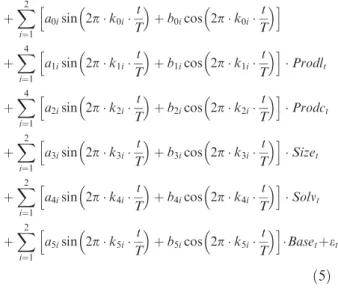
metho-dology described here to our generic Equation 1 and restricting ourselves to only two possible frequencies for all the regressors and to four frequencies for the productivity regressors result in the following general model:
Profitability
¼a0þa1Prodltþa2Prodctþa3Sizetþa4Solvtþa5Base5
þX
2
i¼1
a0isin 2pk0it
T
þb0icos 2pk0it
T h i þX 4 i¼1
a1isin 2pk1it
T
þb1icos 2pk1it
T h i Prodlt þX 4 i¼1
a2isin 2pk2i
t T
þb2icos 2pk2i
t T h i Prodct þX 2 i¼1
a3isin 2pk3i
t T
þb3icos 2pk3i
t T h i Sizet þX 2 i¼1
a4isin 2pk4it
T
þb4icos 2pk4it
T h i Solvt þX 2 i¼1
a5isin 2pk5i
t T
þb5icos 2pk5i
t T
h i
Basetþet
ð5Þ
The interpretation of Equation 5 is that the magni-tude of any fluctuations in the constant term is captured
by nonzero values ofa0iandb0i. Similarly, fluctuations
in the coefficients of explanatory variables are captured
by nonzero values ofajiandbji, wherej= 1, . . ., 5. The
frequencies of the fluctuations in the constant term are
given byk0i, while the frequencies of the fluctuations in
the coefficients of explanatory variables are given bykji,
wherej= 1, . . ., 5.
IV. Data
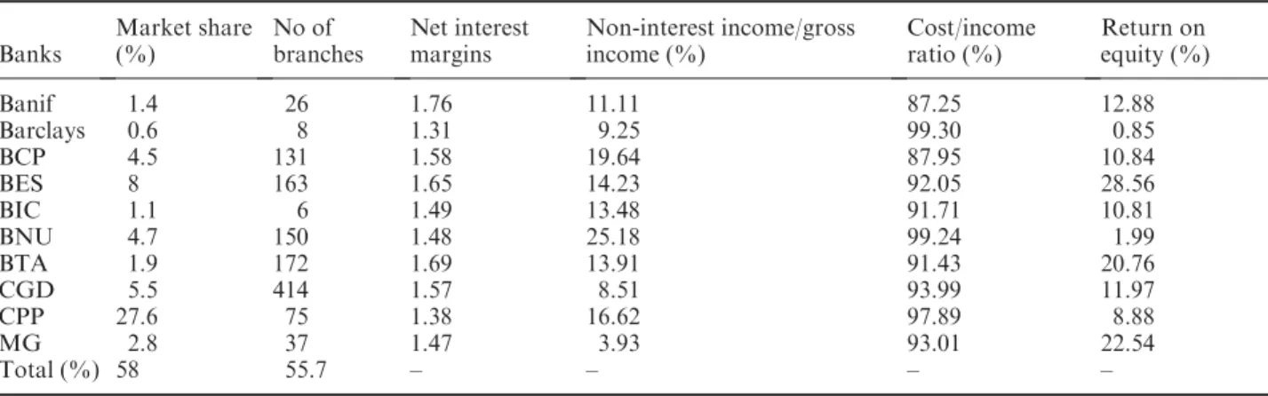
This study uses a balanced-panel database on Portuguese banks from 1990 to 2005, including a total of 160 observations. The banks used in the study and their economic characteristics in 1990 and 2005 are presented in Tables 1 and 2, respectively. The sample includes the main national private banks (BCP and BES), the sole state-owned bank (CGD), the sole mutualist bank (MG) and the only foreign bank (Barclays), which were actively present in the market in all the years of the period under analysis. As can be seen in Table 1, at the beginning of the period ana-lysed, the sample represents 58% of the total market share and 55.7% of all bank branches.
Table 2 shows that at the end of the period examined, the sample represents 70.1% of the total market share and 61.7% of the total bank branches. The net interest margins range from 1.35 to 1.92, a value that resembles the average interest margin observed in the European
market (Goddard et al., 2001, p. 12). The ratio of
noninterest income to gross income ranges from 16.03 to 63.08%, which contrasts with the European values in
the median (Goddardet al., 2001, p. 13). The ratio of
cost to income is higher than the values observed in the
European banking sector (Goddardet al., 2001, p. 15)
while the return on equity is lower.
As mentioned above, the study is concerned with the relationship between the bank’s profitability and its productivity, size, capitalization and portfolio
com-position. The Return on Assets (ROA) and the Return
on Equity (ROE) are used as profitability variables.
The productivity variables are labour productivity (Prodl), measured as the ratio between net income and the number of employees, and capital
productiv-ity (Prodc), measured as the ratio between net income
and the number of branches. Three different size
vari-ables were used, the log of total assets (Sizea), the
formula-1/(total deposits/1 000 000) (Sized) and the
log of bank product (Sizepb). Bank capitalization,
determined as the ratio of between own funds and total assets, and portfolio composition, determined as the ratio between total deposits and total assets,
are represented bySolvandBase, respectively.
All data are in 1995 real terms, converted using the GDP deflator, with the exception of the number of agencies and the number of employees. Table 3 reports descriptive statistics of the variables used in the model, where the heterogeneity of the banks included in sam-ple showed in Tables 1 and 2 can be confirmed.
V. Results
In accordance with the strategy of identification of the Fourier coefficients suggested in Ludlow and Enders (2000), we begin estimating the general model (Equation 5) without the inclusion of the Fourier coefficients, that is, assuming that the resulting coeffi-cients would be invariable.
The first empirical results are revealed to be weak
whenROEis used as a profitability variable. Equally,
of the three size variables used, onlySizedis
statisti-cally significant. To save space, the results are only
Table 1. Characteristics of the bank sample in 1990
Banks
Market share (%)
No of branches
Net interest margins
Non-interest income/gross income (%)
Cost/income ratio (%)
Return on equity (%)
Banif 1.4 26 1.76 11.11 87.25 12.88
Barclays 0.6 8 1.31 9.25 99.30 0.85
BCP 4.5 131 1.58 19.64 87.95 10.84
BES 8 163 1.65 14.23 92.05 28.56
BIC 1.1 6 1.49 13.48 91.71 10.81
BNU 4.7 150 1.48 25.18 99.24 1.99
BTA 1.9 172 1.69 13.91 91.43 20.76
CGD 5.5 414 1.57 8.51 93.99 11.97
CPP 27.6 75 1.38 16.62 97.89 8.88
MG 2.8 37 1.47 3.93 93.01 22.54
Total (%) 58 55.7 – – – –
Table 2. Characteristics of the bank sample in 2000
Banks
Market share (%)
No of branches
Net interest margins
Non-interest income/gross income (%)
Cost/income ratio (%)
Return on equity (%)
Banif 1.6 116 1.83 32.88 95.31 7.27
Barclays 0.05 52 1.61 40.38 94.32 13.04
BCP 20.7 1.221 1.70 40.92 90.19 38.44
BES 10.8 469 1.35 63.08 96.62 18.82
BIC 2.8 121 1.50 17.72 89.96 24.30
BNU 2.5 177 1.56 52.87 98.77 4.33a
BTA 0.07 276 1.76 44.15 95.27 10.66b
CGD 8.3 594 1.62 54.07 92.81 20.54
CPP 18.5 154 1.78 23.82 98.90 2.88b
MG 3.8 259 1.92 16.03 89.86 17.17
Total 70.1 61.7 – – – –
Notes:aIn 2000, the BNU was integrated into the CGD Group.
b
This atypical values are due to BTA’s and CPP’s integration into the Santander Group.
discussed for the model employingROAandSizedas variables of profitability and size, respectively.
With regard to the estimation results without Fourier coefficients, we conclude that, based upon
conventional t-ratios, the constant term (Constant)
and the banks’ portfolio composition (Base) are not
statistically significant explanations for the changes in the banks’ profitability. Therefore, these are excluded from the estimations. The model appears to fit well
with an adjustedR2of 74.6% and anF-statistic that
rejects the joint hypothesis that the coefficients on all
variables are not significantly different from zero.2
These first results without Fourier coefficients confirm the a prioriexpectations that the bank performance
(ROA) is positively explained by the bank labour and
capital productivity (ProdlandProdc), the bank size
(Sized) and the bank capitalization ratio (Solv). Next, we test the existence of nonlinear relationships
among the dependent variableROAand the
explana-tory variables used in the study. In other words, we proceed to identify the particular Fourier coefficients to include in our model. The specification problem of the model now consists in selecting the proper frequencies to include in the Fourier coefficients (when they exist
Table 3. Descriptive statistics of the variables used in the model (1990–2005)
Variables Mean SD Min. Max.
ROA 0.0064 0.0048 -0.0166 0.0179
ROE 0.1349 0.1048 -0.3521 0.5352
Prodl 3.0454 2.4157 -4.5241 12.8048
Prodc 56.8958 53.9621 -112.8874 358.6027
Sizea 13.9296 1.1561 11.3567 16.1486
Sized -2.0841 2.7260 -15.7479 -0.1124
Sizepb 10.2772 1.0887 8.0775 12.5612
Solv 0.0610 0.0292 0.0257 0.1635
Base 0.8426 0.0935 0.5027 0.9543
Notes: The variables have been deflated using GDP deflator with 1995 as a base year.
Table 4. Estimation results (dependent variableROA)
Variables Parameters Coefficients SE t-Ratio
Prodl a1 0.0008083 0.0000898 9.00483
Prodc a2 0.0000589 0.0000049 11.94012
Sized a3 0.0002957 0.0000604 4.89554
Solv a4 0.0187000 0.0046618 4.00407
Sin(w01)*Constant a01 -0.0011860 0.0001690 -7.01778
Cos(w11)*Prodl bl1 0.0002117 0.0000454 -4.66259
Sin(w12)*Prodl a12 0.0002129 0.0000598 -3.55755
Cos(w13)*Prodl b13 0.0002573 0.0000431 5.97020
Cos(wl4)*Prodl b14 0.0002056 0.0000461 4.45474
Sin(w21)*Prodc a21 0.0000108 0.0000024 4.43538
Sin(w22)*Prodc a22 -0.0000146 0.0000024 -6.09532
Cos(w31)*Sized b31 -0.0004914 0.0000684 -7.18558
Cos(w32)*Sized b32 0.0002774 0.0000581 4.77379
Sin(w41)*Solv a41 -0.0104000 0.0027589 -3.78107
Sin(w42)*Solv a42 -0.0085751 0.0027403 -3.12925
Cos(w51)*Base b51 -0.0005987 0.0001852 -3.23210
Sin(w52)*Base a52 -0.0005755 0.0001904 -3.02178
Observations 160
F(4.93)a 1051.497
F(17.93) 303.870
R2-adjusted 0.943
SBC -910.184
Note:aTheF-statistic for the joint hypothesis that the coefficientsa1,a3,a3anda4are equal to 0.
2These results, as well as those for all the other models that useROEand the size variablesSizeaandSizepb, are available on
request from the authors.
and are statistically significant) associated with the var-ious explanatory variables. Following the above-mentioned four-step identification strategy, we obtain the results presented in Table 4.
As can be observed, the introduction of the Fourier coefficients into the model improves the quality of the
adjustment, resulting in an adjustedR2of 94.3%. This
increase in the global significance of the model can
also be verified by theF-statistic associated with the
hypothesis of nullity of the invariable coefficients
(a1=a2=a3=a4= 0), which increased four times
(from 269.4 to 1051.5). The significance is further confirmed by the obtaining of a quite inferior value
forSBC(which decreased from –792.848 to –910.184).
A representation of the residuals from the model with and without Fourier coefficients is shown in Fig. 1.
The comparison confirms the values of SBC, which
are quite favourable relative to the nonlinear model. As mentioned earlier, the tests to the statistic sig-nificance of the Fourier coefficients should not be
made with base in the standard critical values tand
F, but rather in the critical values t* and F* (not
presented, are available on request from the authors).3
Additionally, we do not accept any coefficient whose
inclusion does not result in a decrease of the SBC,
which is a model selection criteria that trades off a reduction in the sum of squared residuals for a more parsimonious model and therefore avoids a possible problem of overfitting in the model. 13 Fourier coeffi-cients were included in the model. The inclusion of Fourier coefficients is accepted even for the regressors that previously had not revealed statistically signifi-cant explanations for the alterations in the
perfor-mance of the banks (Constant and Base), which
means that both present an exclusively nonlinear
rela-tionship with the profitability variable ROA. The
Fourier coefficients included in the model and the
associated frequencies kji are reported in Table 5
below.
As we can see, all the variables (with the exception of the constant term) have more than one single frequency
associated. The variableProdlhask11= 14,k12= 5,
k13= 2 andk14= 13 associated with coefficientsb11,
a12,b13andb14, respectively;Prodchask21= 10 and
k22= 18 associated witha21anda22;Sizedhask31= 1
and k32 = 8 associated with b31 and b32; Solv has
k41= 8 andk42= 11 associated witha41anda42; and
Basehask51= 30 andk52= 16 associated withb51and
a52. Using the t*-test statistic, almost all the Fourier
coefficients are significantly different from 0 at the 1%
level. The exceptions area12,a42,b51anda52, which are
only statistically significant at the 5% level.
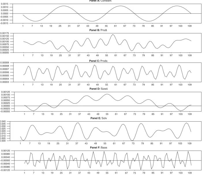
An important aspect to point out is the behaviour of the coefficients of the model along the sample. As can be seen through the graphic representation of the estimated coefficients (Fig. 2), all the variables present a nonlinear relationship with profitability. Focusing our attention on the variables with a constant part in the associated coefficients, we can see that, although Without Fourier coefficients – Resids1/With
Fourier coefficients – Resids2
–0.0100 –0.0075 –0.0050 –0.0025 0.0000 0.0025 0.0050 0.0075
1 11 21 31 41 51 61 71 81 91 101 Resids1 Resids2
Fig. 1. Residuals of the estimation – model
Table 5. Fourier coefficients of the model
a01 b11 a12 b13 b14 a21 a22
Coefficient -0.001186 -0.000212 -0.000213 0.000257 0.000206 0.000011 -0.000015
t-Ratio -7.02 -4.66 -3.56 5.97 4.45 -4.44 -6.10
Frequency (kji) k01= 3 k11= 14 k12= 5 k13= 2 k14= 13 k21= 10 k22= 18
b31 b32 a41 a42 b51 a52
Coefficient -0.000491 0.000277 -0.010400 -0.008575 -0.000599 -0.000575
t-Ratio -7.19 4.77 -3.78 -3.13 -3.23 -3.02
Frequency (kji) k31= 1 k32= 8 k41= 8 k42= 11 k51= 30 k52= 16
3Note thatF* does not correspond to the critical value associated to the hypothesis of nullity of all the Fourier coefficients but
instead to the critical value associated to the test of nullity of the pairs sin/cos of the Fourier coefficients (aji=bji= 0).
the coefficients ofProdl,ProdcandSolvalways con-tinue to assume positive values along the sample, the
variableSizedhas a coefficient that assumes negative
values in some parts of the sample. This continues to be in agreement with the remaining empirical evidence that, as mentioned in a synthesis by Naceur and Goaied (2001), has been supporting the existence of a positive or negative effect on the relationship between the bank’s size and its profitability.
Another important aspect to mention is the consis-tency presented by the Fourier model. The fact that the introduction of the Fourier coefficients into the model in order to not cause a significant alteration in
the estimated values of the coefficientsa1,a2,a3anda4
means that the model has a high degree of consistency. With reference to the model (Table 4), one may then rank the statistically significant explanatory variables
in terms of their contribution to explaining the banks’ profitability according to the absolute values of their
t-ratios. In so doing and taking into consideration that
the relevant analysis concerns the coefficients asso-ciated with the explanatory variables that have a con-stant (invariable) part, one finds the following ranking (in decreasing order of importance) for the more impor-tant determinants: (1) capital productivity, (2) labour productivity, (3) bank size and (4) bank capitalization.
VI. Conclusion
The main objective of this study is to analyse the deter-minants of banks’ profitability in the Portuguese bank-ing sector durbank-ing the period 1990 to 2005. This article extends the established literature on modelling the
Panel A: Constant
–0.0015 –0.0010 –0.0005 0.0000 0.0005 0.0010 0.0015
Panel B: Prodl
0.00000 0.00025 0.00050 0.00075 0.00100 0.00125 0.00150 0.00175
Panel C: Prodc
0.00003 0.00004 0.00005 0.00006 0.00007 0.00008 0.00009
Panel D: Sized
–0.00050 –0.00025 0.00000 0.00025 0.00050 0.00075 0.00100 0.00125
Panel E: Solv
0.000 0.005 0.010 0.015 0.020 0.025 0.030 0.035 0.040
Panel F: Base
–0.00120 –0.00080 –0.00040 –0.00000 0.00040 0.00080 0.00120
1 7 13 19 25 31 37 43 49 55 61 67 73 79 85 91 97 103 109 1 7 13 19 25 31 37 43 49 55 61 67 73 79 85 91 97 103 109 1 7 13 19 25 31 37 43 49 55 61 67 73 79 85 91 97 103 109 1 7 13 19 25 31 37 43 49 55 61 67 73 79 85 91 97 103 109 1 7 13 19 25 31 37 43 49 55 61 67 73 79 85 91 97 103 109 1 7 13 19 25 31 37 43 49 55 61 67 73 79 85 91 97 103 109
Fig. 2. Estimated coefficients of the model
banks’ profitability by applying Fourier coefficients to detect for possible nonlinearities between the perfor-mance variables and the explanatory variables. In so doing, we verify that the introduction of the Fourier coefficients in the analysis quite improved the quality of the adjustments, the need to accept the existence of nonlinear relationships among the variables involved in the study thus becoming evident.
The findings of this article therefore suggest that the best performing banks in the Portuguese banking sector are those which have endeavoured to improve their capital and labour productivity, those which have main-tained a high dimension and, finally, those which have been able to reinforce their capital structure. Despite not having a variable for market concentration, the statis-tical significance of market share suggests that the SCP is supported, validating Molyneux and Forbes (1995).
References
Agostino, M., Leonida, L. and Trivieri, F. (2005) Profits persistence and ownership: evidence from the Italian banking sector,Applied Economics,37, 1615–21. Altunbas, Y., Gardener, E., Molyneux, P. and Moore, B.
(2001) Efficiency in European banking, European Economic Review,45, 1931–55.
Barros, C., Ferreira, C. and Williams, J. (2007) Analysing the determinants of performance of the best and worst European banks: a mixed logit approach, Journal of Banking and Finance,31, 2189–203.
Becker, R., Enders, W. and Hurn, A. (2002) A general test for time-dependence in parameters,Journal of Applied Econometrics,19, 899–906.
Berger, A. and Humphrey, D. (1997) Efficiency of financial institutions: international survey and directions for future research, European Journal of Operational Research,98, 175–212.
Berger, A., Leusner, J. and Mingo, J. (1997) The efficiency of
bank branches, Journal of Monetary Economics,
40, 141–62.
Berger, A. and Mester, L. (1997) Inside the black box: what explains differences in the efficiency of financial institu-tions,Journal of Banking and Finance,21, 895–947. Berger, A. and Mester, L. (2003) Explaining the dramatic
changes in performance of US banks: technological change, deregulation, and dynamic changes in competi-tion,Journal of Financial Intermediation,12, 57–95. Das, A. and Das, S. (2007) Scale economies, cost
comple-mentarities and technical progress in Indian banking: evidence from Fourier flexible functional form,Applied Economics,39, 565–80.
Enders, W. and Hoover, G. (2003) The effect of robust growth on poverty: a non-linear analysis, Applied Economics,35, 1063–71.
Enders, W. and Sandler, T. (2001) Non-linear effects and
improved estimates of transnational terrorism,
Unpublished Paper.
Evanoff, D. and Fortier, D. (1988) Reevaluation of the structure-conduct-performance paradigm in banking,
Journal of Financial Service Research,1, 249–60. Gallant, A. (1981) On the bias in flexible functional forms
and essentially unbiased form: the Fourier flexible form,Journal of Econometrics,46, 229–45.
Gallant, A. (1982) Unbiased determination of production technologies,Journal of Econometrics,20, 285–324. Gilbert, R. (1984) Bank market structure and competition,
Journal of Money, Credit and Banking,16, 617–45. Goddard, J., Molyneux, P. and Wilson, J. (2001)European
Banking: Efficiency, Technology and Growth, John Wiley and Sons, New York.
Haggestad, A. and Mingo, J. (1977) The competition condi-tion of US banking markets and the impact of struc-tural reforms,Journal of Finance,32, 649–61.
Huang, T. and Wang, M. (2004) Estimation of scale and scope economies in multiproduct banking: evidence from the Fourier flexible functional form with panel data,Applied Economics,36, 1245–53.
Ludlow, J. and Enders, W. (2000) Estimating non-linear
ARMA models using Fourier coefficients,
International Journal of Forecasting,16, 333–47. Maudos, J. (2001) Rendabilidad, Estructura de Mercado y
Efficiencia en la Banca,Revista de Economia Aplicada, 25, 193–207.
Mitchell, K. and Onvural, N. (1996) Economies of scale and scope at large commercial banks: evidence from the Fourier flexible functional form, Journal of Money, Credit and Banking,28, 178–99.
Molyneux, P. and Forbes, W. (1995) Market structure and performance in European banking,Applied Economics, 27, 155–9.
Naceur, S. and Goaied, M. (2001) The determinants of the Tunisian deposit banks performance,Applied Financial Economics,11, 317–9.
Rhoades, S. (1982) Welfare loss, redistribution effect and restriction of output due to monopoly, Journal of Monetary Economics,9, 375–87.
Shen, C. (2005) Cost efficiency and banking performances in a partial universal banking system: application of the panel smooth threshold model,Applied Economics,37, 993–1009.
Smirlock, M. (1985) Evidence of the (non) relationship between concentration and profitability in banking,
Journal of Money, Credit and Banking,17, 69–83. Spellman, L. (1981) Commercial banks and the profit of
saving and loans markets,Journal of Bank Research, 12, 32–9.