Hysteresis effects under CIR interest rates

Texto

(1)Lancaster University Management School Working Paper 2010/031. Hysteresis Effects under CIR Interest Rates. Jose Carlos Dias and Mark Shackleton The Department of Accounting and Finance Lancaster University Management School Lancaster LA1 4YX UK. © Jose Carlos Dias and Mark Shackleton All rights reserved. Short sections of text, not to exceed two paragraphs, may be quoted without explicit permission, provided that full acknowledgement is given. The LUMS Working Papers series can be accessed at http://www.lums.lancs.ac.uk/publications/ LUMS home page: http://www.lums.lancs.ac.uk/.

(2) Hysteresis Effects under CIR Interest Rates∗ Jos´ e Carlos Dias† Finance Research Center (FRC/ISCTE) and ISCAC Business School, Quinta Agr´ıcola, Bencanta, 3040-316 Coimbra, Portugal. Tel: +351 239 802185. Fax: +351 239 445445. E-mail: jdias@iscac.pt. Mark B. Shackleton Department of Accounting and Finance, Lancaster University Management School, Lancaster, LA1 4YX, UK. Tel: +44 1524 594131. Fax: +44 1524 847321. E-mail: m.shackleton@lancaster.ac.uk. ∗. The authors thank the helpful comments and suggestions addressed by three anonymous referees. The. authors thank also João Pedro Nunes, José Paulo Esperan¸ca, Mohamed Azzim Gulamhussen, as well as the 9th Real Options Group Conference participants (Paris 2005) and finance seminar participants at ISCTE Business School (Lisbon 2005) for helpful comments on a previous draft of the paper. Any remaining errors are solely our responsibility. Dias gratefully acknowledges the financial support by FCT’s grant number PTDC/EGE-ECO/099255/2008. † Corresponding author..

(3) Hysteresis Effects under CIR Interest Rates Abstract. Most decision making research in real options focuses on revenue uncertainty assuming discount rates remain constant. However, for many decisions revenue or cost streams are relatively static and investment is driven by interest rate uncertainty, for example the decision to invest in durable machinery and equipment. Using interest rate models from Cox et al. (1985b), we generalize the work of Ingersoll and Ross (1992) in two ways. Firstly, we include real options on perpetuities (in addition to zero coupon cash flows). Secondly, we incorporate abandonment or disinvestment as well as investment options, and thus model interest rate hysteresis (parallel to revenue uncertainty in Dixit (1989a)). Under stochastic interest rates, economic hysteresis is found to be significant, even for small sunk costs.. Keywords: Finance; Real options; Interest rate uncertainty; Perpetuities; Investment hysteresis.

(4) 1. Introduction The capital theory of investment has typically ranged from models where investment is costlessly reversible to models where investment is completely irreversible. The case of costlessly reversible investment occurs when there is no difference between the price at which the firm can purchase capital projects and the price at which it can sell. Thus, with perfect reversibility the wedge between the investment cost and the divestment proceeds is zero and the optimal investment policy of a firm maintains the marginal revenue product of capital equal to the Jorgenson (1963) user cost of capital. The case of costlessly reversible investment is unrealistic since it is not expected that a firm can divest at no cost. Most investment expenditures are at least in part irreversible, i.e., should market conditions change adversely there are sunk costs that cannot be totally recouped. Although some investments can be reversed, the majority of them are at least partly irreversible because firms cannot recover all their investment costs. Furthermore in some cases, additional costs of decommissioning machinery may exist. Since most of capital expenditure is firm or industry specific, these should be considered with a sunk cost, but even if these capital expenditures are not firm or industry specific, they could not be totally recovered due to the “lemons” problem of Akerlof (1970). Hence, major investment costs are in a large part irreversible. As a result, the full cost of investment must be the sum of two terms: the cost of investment itself (a direct cost of investment) and the opportunity cost value of the lost option (an indirect cost of investment). An extensive literature has shown how this opportunity cost on the lost option can be evaluated. It has also demonstrated that its value is extremely sensitive to uncertainty and can have a large impact on investment spending.1 At the other opposite extreme, lies the case of completely irreversible investment when the sale price of capital is zero, i.e., the firm cannot recoup any fraction of the initial investment cost. For the sake of simplicity, the extreme assumption that resale of capital goods is 1. See Pindyck (1991) and Dixit (1992) for an overview of the literature. Dixit and Pindyck (1994) provide. an excellent revision of the various approaches and applications. A complementary survey may be found in Caballero (1999).. 1.

(5) impossible, i.e. divestment proceeds are zero, was initially introduced by Arrow (1968) and employed in the literature on optimal investment under uncertainty. This assumption is more realistic since in many economic situations the sale of capital invested cannot be accomplished at any price.2 However, the most common case is characterized by investments with costly reversibility in which a firm can purchase capital at a given price (by paying an investment cost I) and sell capital at a lower price (by receiving the divestment proceeds I), i.e., there is a fraction α of the invested capital, α = I/I (with 0 < α < 1), that a firm can recoup when divesting.3 Examples of an analysis for reversible investment decisions include, among others, Dixit (1989a), Abel et al. (1996), Abel and Eberly (1996), Kandel and Pearson (2002), Keswani and Shackleton (2006), and Tsekrekos (2010) in which capital can be suspended at a cost since only a fraction of the entry value can be recovered on exit.4 Decisions made under an uncertain environment where it is costly to reverse economic actions lead to an intermediate range, called the hysteretic band, where continuation is the optimal policy until some threshold is reached. Several models of entry and exit decisions have shown that the range of inaction can be remarkably large (see, for example, Brennan and Schwartz (1985), Dixit (1989a,b), and Abel and Eberly (1996)). The economic hysteresis effect is also found to be wide in the optimal consumption and portfolio choice literature (see, for instance, Constantinides (1986)). Therefore, such effect seems to be extremely relevant for many economic applications. Since interest rates are also an important determinant of investment and divestment decisions it is important to analyze the economic hysteresis effect provoked by interest rate 2. Moreover, there may even exist cases where additional costs of closing a project may exist, such as the. cases of a copper mine or a nuclear power station where environmental costs may have to be supported. 3 α = 0 represents the case where investment is completely irreversible, while α = 1 stands for the case of costlessly reversible investment. For the cases where it is necessary to a pay a lump–sum cost to exit the disinvestment proceeds I is of negative sign. 4 It should be noted that in Dixit (1989a) model firms can decide to suspend operations but have to pay a lump-sum exit cost l to do so. However, the case in which a part of the entry cost, k, can be recovered on exit can easily extended to the costly reversible investment case by changing the sign of l.. 2.

(6) uncertainty. Our paper relates to those that examine the investment decision problem under stochastic interest rates, including, among others, Ingersoll and Ross (1992), Ross (1995), Lee (1997), Alvarez and Koskela (2006), and Dias and Shackleton (2009). However, none of these papers consider abandonment options and thus hysteresis modelling under stochastic interest rates is not previously addressed in the literature. Most decision making research in this so called real options literature, focuses on revenue uncertainty assuming discount rates remain constant. For many decisions, however, revenue or cost streams are relatively static and investment is driven by interest rate uncertainty, for example the decision to invest in durable machinery and equipment. Using interest rate models in a Cox Ingersoll Ross economy (see Cox et al. (1985a,b)), we generalize the work of Ingersoll and Ross (1992) in two ways. Firstly in addition to zero coupon cash flows, we include real options on perpetuities. Secondly, we incorporate suspendment or divestment as well as investment options, and thus model interest rate hysteresis (parallel to the revenue uncertainty in Dixit (1989a)). Our results allow us to conclude that when there is some interest rate uncertainty, hysteresis levels emerge very quickly even for very small reversibility costs. This means that apart from the output price uncertainty (see, for example, Dixit (1989a)), interest rate uncertainty also plays a critical role for widening the hysteretic band. When interest rates fall, firms make durable investments, that is to say that they switch from cash (an immediate asset) to longer lived assets with cash flows further ahead in time. When interest rates rise, they will stop undertaking any durable projects. Furthermore, if flexibility exists they will also try and reverse the investment process, i.e., divest from projects with long lived cash flows into those with more immediate flexibility. The outline of this paper is as follows. Section 2 describes the firm’s optimisation problem and policy. Section 3 presents the interest rate process in a CIR economy and solutions for the value components. Section 4 provides a concrete numerical example and results for the economic hysteresis problem, while section 5 concludes.. 3.

(7) 2. The firm’s policy The situation for the firm that we consider is that it can invest I at any time and receive a perpetuity P (r) (a project) with constant unit cash flow rate, although the projects cash flows are fixed, its perpetuity value (negatively related to rates) is stochastic because the interest rate r used to discount the perpetual flows can change. Investment in this perpetual project will be triggered when interest rates are low (high perpetuity value) and in particular at a critical level r. Having invested and secured the constant stream of investment returns, a divestment option is still valuable because interest rates may change again and with it the perpetuity value. In particular if rates rise and the perpetual project’s worth falls, there may be a lower value at which it is worth suspending the project in favour of regaining cash of value I = αI (α < 1). This occurs when interest rates peak (and perpetuity values dip) at r. We require value functions and notation for the active project (with perpetuity) which has the option to shut, and the inactive project (without flow) but with the option to open. These are labelled F1 (r) + P (r) and F0 (r) respectively. All three components will satisfy an ordinary differential valuation equation (which is derived in the next section) but with different cash flow conditions. Investment will be triggered as interest rates r fall to the lower investment trigger r whilst divestment will be triggered as rates rise to the upper trigger r (r > r), this is captured by the following value matching conditions F0 (r) + I → F1 (r) + P (r) F0 (r) + I ← F1 (r) + P (r). Thus, an idle firm invests when interest rates fall to r and an operating firm will divest once the interest rates rise to r. A useful value to define is the value premium V of active to idle firms, this depends on current rates r V (r) = F1 (r) + P (r) − F0 (r) 4. (1).

(8) and the value matching conditions can be coupled with two smooth pasting (first order) conditions V (r) = I − P (r), V 0 (r) = 0, V (r) = I, V 0 (r) = 0.. (2). The range r, r is the hysteretic band of the problem since idle firms do not invest and operating firms do not suspend within this intermediate level of interest rates. Although well discussed for income uncertainty, hysteresis problems have not been discussed for interest rate uncertainty. Furthermore although similar problems have been solved for geometric Brownian processes, in this paper we can solve this problem with mean-reverting processes and compare the range of hysteresis. As we show later, one important conclusion is that this range of inaction has a tendency to be even higher when a mean reversion feature is introduced.. 3. CIR rate dynamics Consider (at time t = t0 ) a CIR economy in which EQ t0 denotes expectations under the martingale (or risk-neutral) probability measure Q, with respect to the risk-adjusted process for the instantaneous interest rate rt √ drt = [κθ − (λ + κ)rt ]dt + σ rt dWtQ .. (3). The parameter that determines the speed of adjustment (reversion rate) is κ > 0 the intensity with which the interest rate is drawn back towards a long–run mean, another variable given by θ > 0 the long–run mean of the instantaneous interest rate (asymptotic interest rate). Furthermore σ is the volatility of the process, λ is the market risk parameter5 , rt is the instantaneous interest rate and WtQ is a standard Brownian motion under Q. This model nests the simpler one used by Ingersoll and Ross (1992). 5. Positive premia will exist if λ < 0. It should be emphasized that although risk premiums for interest. rates may be introduced, they cannot be observed or measured separately (see the detailed discussion in Dias and Shackleton (2005, Section 2) as well as the references contained therein).. 5.

(9) One of the key issues with this square-root diffusion is the role played by the term κθ, which has important implications for capture of the interest rate process r at a value of zero.6 Remembering that the variance of the process rσ 2 dt locally vanishes at r = 0, three important conditions are of particular interest: (i) κθ = 0 : the process is not mean reverting at all and the level r = 0 is an absorbing barrier. Thus, when it hits 0 it remains constant forever. (ii) 0 < κθ < 12 σ 2 : the process is mean reverting. The strength of the reversion force is not great enough however to prevent the process reaching zero but it is strong enough to retrieve it from zero. Thus r = 0 is a reflecting boundary where the deterministic drift can lift it back above zero, until the next time zero is encountered. (iii) 21 σ 2 ≤ κθ : here the strength of the mean reversion force is great enough to ensure that the process never reaches the zero level. Furthermore a process starting at r = 0 will be drawn away from that level never to return. Thus under this condition the process stays strictly positive once positive. Under all conditions the interest rate remains non–negative but the first case, with a chance that future rates will get stuck at zero, is pathological in the sense that perpetuities cannot be valued.. 3.1. CIR general claims Following Cox et al. (1985a,b), the price of a general interest rate claim F (r, t) with cash flow rate C(r, t) satisfies the following partial differential equation. ∂F (r, t) ∂F (r, t) ∂F (r, t) 1 2 ∂ 2 F (r, t) σ r + κ(θ − r) + − λr − rF (r, t) + C(r, t) = 0. 2 2 ∂r ∂r ∂t ∂r 6. See Feller (1951) for a complete description of the boundary classifications.. 6. (4).

(10) The price of a zero coupon bond Z(r, t, T ) satisfies this equation with C(r, t) = 0 subject to the boundary condition Z(r, T, T ) = 1.7. 3.2. Particular integral Since it is not time dependent, the value of a perpetuity P (r) that pays coupons at a constant unit rate C(r) = 1 solves this last equation with. ∂F (r,t) ∂t. = 0. There are several. ways8 to recover this value (see Delbaen (1993) and Geman and Yor (1993)) but a useful formulation given by Delbaen (1993, pg. 129) is. P (r) =. ω Φ1 (1, β, γ, x, y) κθ. (5). where Φ1 is the degenerate hypergeometric function (also known as one of the confluent Horn series). Since this function is one solution to the ordinary differential equation, it is known as the particular integral. Appendix B shows the series expansion of this perpetuity function (and its first derivative) as well as its arguments. Most generally other functions that also solve the ordinary differential equation (ode) with no coupon flows must now be sought and these will represent the option components.. 3.3. Complementary functions Specialising to this time homogenous situation gives a simpler ode that determines the perpetual option to invest in or divest from a project. Furthermore for the options themselves no cash flows are present so C(r) = 0 7. For completeness sake, the value function of this zero bond is listed in Appendix A with the other. components. 8 Another way to retrieve the perpetuity value is via a continuum of zeros Z ∞ P (r) = Z(r, 0, t)dt 0. and there are also complex integral methods.. 7.

(11) 1 2 ∂ 2 F (r) ∂F (r) ∂F (r) σ r + κ(θ − r) − λr − rF (r) = 0. 2 ∂r2 ∂r ∂r. (6). The two solutions to this equation are known as complementary functions for the prior ode. One will represent the option value of an idle firm F0 (r), and the other an active firm F1 (r) (but without the perpetuity P (r) which is the particular integral solution of the ode including the coupon term). What determines the difference between the two contingent solutions and the options they represent is their boundary conditions. Both complementary functions are given by series solutions of known type but with different forms. The solutions for an idle firm and an active firm can be given respectively by (the proof is shown in Appendix C). F0 (r) = C1 ev0 r M (a0 , b, z0 ) + C2 ev0 r U (a0 , b, z0 ). (7). F1 (r) = C3 ev1 r M (a1 , b, z1 ) + C4 ev1 r U (a1 , b, z1 ). (8). with. ω = v0,1 = a0,1 = b = z0,1 =. £. ¤1/2 (κ + λ)2 + 2σ 2 κ+λ∓ω 2 µσ ¶ κθ κ+λ 1∓ σ2 ω 2κθ σ2 2ω ± 2r σ. (9a) (9b) (9c) (9d) (9e). and where C1−4 are constants to be determined from boundary conditions, M (a, b, z) is the Kummer confluent hypergeometric function as given by Slater (1960, Equation 1.1.8), Abramowitz and Stegun (1972, Equation 13.1.2) or Lebedev (1972, Equation 9.9.1), and finally U (a, b, z) is the Tricomi confluent hypergeometric function (or Kummer confluent 8.

(12) hypergeometric function of the second kind) as defined by Slater (1960, Equation 1.3.5), Abramowitz and Stegun (1972, Equation 13.1.3) or Lebedev (1972, Equation 9.10.4).9. 3.4. Boundary conditions We know that the option of activating an idle firm should be nearly worthless for high interest rate levels. Since ev0 r M (a0 , b, z0 ) is an increasing function of r, we must set C1 = 0. Similarly, the option of shutting an operating project should be nearly worthless for low interest rate levels. Thus, we must set C4 = 0 since ev1 r U (a1 , b, z1 ) is a decreasing function of r. As a result, the expected net present value in the idle state with the option to open is. F0 (r) = C2 ev0 r U (a0 , b, z0 ). (10). and the option to switch out of the perpetuity is. F1 (r) = C3 ev1 r M (a1 , b, z1 ).. (11). 3.5. First order conditions To determine optimality, we need to use the first derivative of the functions (10) and (11) as well as that of the perpetuity value. To compute the derivative of U (a, b, z) with respect to z we use the definition of Slater (1960, Equation 2.1.24), Abramowitz and Stegun (1972, Equation 13.4.21) or Lebedev (1972, Equation 9.10.12). Similarly, we use definition of Slater (1960, Equation 2.1.1), Abramowitz and Stegun (1972, Equation 13.4.8) or Lebedev (1972, Equation 9.9.4.) to compute the derivative of M (a, b, z) with respect to z. These are shown in Appendixes D and E, respectively. These functional forms (which depend on C2 , C3 ) can 9. Both functions are available as built-in functions in Mathematica with the call Hypergeometric1F1(a,b,z). and HypergeometricU(a,b,z), respectively.. 9.

(13) be applied to the thresholds at which action is taken r, r to ensure smooth pasting of the solutions either side of the boundary10. ∂F1 (r) ∂P (r) ∂F0 (r) = + ∂r ∂r ∂r ∂F0 (r) ∂F1 (r) ∂P (r) = + . ∂r ∂r ∂r Thus solution of the two sided control problem rests on determination of the two embedded constants C2 , C3 and two thresholds r, r that jointly solve these first order conditions along with the two value matching conditions.. 4. Numerical Example In our numerical analysis we will consider a CIR economy with parameter values κ = 0.2339, θ = 0.0808, σ = 0.0854, and λ = 0 taken from the empirical work of Chan et al. (1992). We will consider also a higher volatility level (σ = 0.30) for comparative purposes. In addition, we use an investment cost of I = 10 and we establish three degrees of reversibility, α = 0.25, α = 0.50 and α = 0.75. We also present the case of perfect reversibility, α = 1, to illustrate the limiting case. The case where α = 0 is also illustrated since it falls in the single investment strategy situation. Table 1 presents both upper and lower interest rate thresholds for the entry and exit problem under CIR interest rates for the set of parameters defined above. 10. Smooth pasting ensures that the rate of return on the firm is the same before and after the transition. (see, for instance, Shackleton and Sødal (2005)).. 10.

(14) Table 1: Upper and lower interest rate thresholds for the entry and exit problem under CIR interest rates. σ = 0.0854 α 0.00 0.25 0.50 0.75 1.00. r 0.0723 0.0723 0.0723 0.0723 0.1000. σ = 0.30. r +∞ 0.7098 0.3969 0.2375 0.1000. r 0.0238 0.0238 0.0244 0.0288 0.1000. r +∞ 0.9328 0.5505 0.3416 0.1000. This table shows upper and lower interest rate thresholds for the entry and exit problem under CIR interest rates with an investment cost I = 10 for different ratios of the disinvestment proceeds to the investment costs (i.e., α = I/I = {0.00, 0.25, 0.50, 0.75, 1.00}) and different interest rate volatilities (i.e., σ = {0.0854, 0.30}). CIR parameters: κ = 0.2339, θ = 0.0808 and λ = 0.. For α = 0, an active firm never shuts its project, since the cash flow never becomes negative. Thus, the corresponding lower thresholds indicate the interest rate level that will induce an idle firm to enter in a project and continue its operations forever since the option to shut down is worthless. For example, considering the base case volatility level and I = 10 it would be necessary for the interest rate to fall to 7.23% to induce an idle firm to invest once for ever. At this rate level, the firm will change the full cost of investment (i.e. option to invest plus investment cost) for a project paying a perpetuity. For the same set of parameters, but with no mean reversion the trigger point is at a lower level of 1.94%. Therefore, with mean reversion firms are induced to invest sooner. Our numerical analysis allow us to conclude that: (i) for a given level of volatility the lower threshold falls as the investment cost rises; and (ii) for a given investment cost level the lower trigger point falls as the volatility level rises. The case where 0 < α ≤ 1 corresponds to the one where idle firms are induced to invest if the interest rate value falls to a sufficient low level, but they own an option to suspend later if interest rates rise to very high values and return to the idle state. Once the project is suspended, the firm owns an option to reinvest again if interest rates reverse to low levels again. We can now evaluate the size of the no–action region.. 11.

(15) 14 12 10. V. 8 6 4 2 0 0.0. 0.1. 0.2. 0.3. 0.4. 0.5. Interest rate. Figure 1: Determination of the numerical upper and lower thresholds. CIR parameters for the base case (mean reversion): κ = 0.2339, θ = 0.0808, λ = 0 and σ = 0.0854. CIR parameters for the special case (no mean reversion): κ = θ = λ = 0 and σ = 0.0854. I = 10 and α = 0.5. Solid line: mean-reverting case. Dashed line with short dashes: no mean-reverting case. Dashed line with long dashes: value matching condition at r (i.e., V (r) = I = 10) and value matching condition at r (i.e., V (r) = I = α I = 5).. Considering a volatility level of σ = 0.0854, an investment cost of I = 10 and α = 0.50, the lower and upper interest rate thresholds are, respectively, r = 7.23% and r = 39.69%, which originates a range of inaction of 32.46% (r − r). Under the no mean-reverting case the lower and upper trigger points are respectively r = 1.99% and r = 26.41%, which gives a lower range of inaction of 24.42%. Figure 1 depicts this example graphically. It is also clearly to see that in the mean-reverting case both thresholds have risen but the hysteretic range is wider. The corresponding Marshallian trigger points would be Mr = 1/I = 10% and Mr = 1/I = 20%, giving a band of inaction of only 10% = Mr − Mr . Our lower trigger point is approximately 28% below the Marshallian investment threshold (80% below for the case with no mean reversion) and our upper trigger point is approximately 98% above the corresponding Marshallian exit point (32% for the no mean-reverting case). 12.

(16) Therefore, similar to other results found in the real options literature (e.g., Brennan and Schwartz (1985), Dixit (1989a,b), and Abel and Eberly (1996)), uncertainty and the embedded option values are responsible for the remarkably large hysteretic band.. 4.1. Robustness The valuation of a real investment project and the rule for determining the optimal timing of investment both depend critically on the stochastic process assumed for the relevant state variable of the project. Based on the above observations about the investment trigger points, we may conclude that if the true generating rate process is of a mean-reverting CIR type, then a decison rule based on a na¨ıve Marshallian analysis induces premature investment (i.e., when interest rates are too high), whereas a real option model based on CIR diffusion without mean reversion induces investment too late (i.e. when interest rates are too low). These results are consistent with the arguments of Dias and Nunes (2010), and Pinto et al. (2009) who have concluded that the incorrect specification of the stochastic process to be used leads to underinvestment through post-optimal exercise, thus exposing a firm to significant errors of analysis. Tsekrekos (2010) presents also similar conclusions when comparing a firm’s entry and exit decisions when the output equilibrium price follows an exogenous mean-reverting process with the decisions of a firm under the usually employed assumption of lognormally distributed output price, as presented by Dixit (1989a). We conclude that the lower trigger point for the single investment strategy (i.e., without the exit option) and the combined entry and exit strategy are equal for the volatility level of σ = 0.0854 and all α parameters (the exception is obviously α = 1). This implies that the firm’s option to shut down later if interest rates start rising for very high levels is almost worthless for moderate volatility levels. For higher levels of volatility, however, this option has some, though not too pronounced value. If we compare the upper trigger points between the single divestment strategy (i.e. without the re–entry option) and the combined strategy, the differences would be much more significant. These differences come from the value of the re–entry option that is owned by 13.

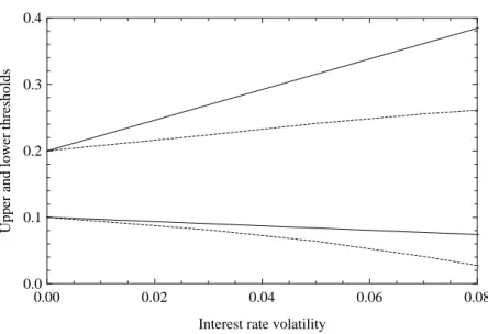
(17) the firm. There is an economic interpretation of this fact. When a firm invests in a project and has an option to shut down in the future, the divestment proceed’s present value is very small because the prospect of closing its operations is sufficiently far in the future and higher discount rates lie between now and that time. As a result, the impact on the lower trigger point is very small. However, when a firm is operating and decides to shut down its activity, it will immediately receive the divestment value, which gives a bigger present value and justifies the greater differences between the two upper trigger points. This is also consistent with results of Keswani and Shackleton (2006) that show a project’s option value increases with incremental levels of investment and divestment flexibility. We know that it is extremely complicated to analyze analytically the impact of the σ parameter on the optimal trigger points. However, we can resort to further numerical results to highlight its effects. Figure 2 presents the impact on the entry and exit thresholds as the volatility rises. Considering I = 10, α = 0.50, and λ = 0, clearly, there is a tendency for a wider range of inaction as the volatility rises. When interest rates are high the economy tends to slow down and borrowers will require less capital. As a result, interest rates have a tendency to decline (mean reversion tends to imply a negative drift). Thus, firms are more reluctant to suspend operations and the upper threshold has a tendency to rise when compared with the no mean–reverting case. When interest rates are at low levels, borrowers demand more funds and interest rates tend to rise (mean reversion tends to imply a positive drift). Since interest rates are at low interest rate levels they are not expected to fall even more. Thus, firms are induced to invest before the likely rise in the interest rate and, as a result, the lower trigger point with mean reversion tends to be higher than the one with no mean reversion. In summary, we can draw the following conclusions from our numerical example: (i) for a given level of volatility and investment cost the lower threshold rises and the upper threshold falls as the α parameter rises (i.e., the divestment proceeds rises). Thus, the hysteretic band will be narrower. We also conclude that when there is any interest rate uncertainty, the hysteresis level emerges very quickly even for very small reversibility costs; (ii) for a given 14.

(18) Upper and lower thresholds. 0.4. 0.3. 0.2. 0.1. 0.0 0.00. 0.02. 0.04. 0.06. 0.08. Interest rate volatility. Figure 2: Entry and exit thresholds as functions of interest rate volatility. CIR parameters for the base case (mean reversion): κ = 0.2339, θ = 0.0808 and λ = 0. CIR parameters for the special case (no mean reversion): κ = θ = λ = 0. I = 10 and α = 0.5. Solid line: mean-reverting case. Dashed line: no mean-reverting case.. volatility level and α parameter both the lower and upper trigger points fall as the investment cost rises; and (iii) for a given investment cost and α parameter the optimal lower trigger point falls and the upper threshold rises as volatility rises, thus originating a wider range of inaction.. 5. Conclusions We model the investment hysteresis problem under stochastic interest rates using a tractable form of interest rate uncertainty and describe the sensitivity of the interest rate band to the model parameters. We do this to analyze the beneficial effects of waiting to invest in the presence of uncertainty as well as to shed light on the macro influence of interest rate changes on investment policies. Our results allow us to conclude that when there is some level of interest rate uncertainty, the hysteresis level emerges very quickly even for very small investment costs. This means 15.

(19) that apart from output price uncertainty (see, for example, Dixit (1989a)), interest rate uncertainty also plays a critical role for determining the hysteretic band. When interest rates fall, firms make durable investments, that is to say that they switch from cash (an immediate asset) to longer lived assets with cash flows further ahead in time. When interest rates rise, they will stop undertaking any durable projects. Furthermore, if flexibility exists they will also try and reverse the investment process, i.e. divest away from projects with long lived cash flows into projects with more immediate payoffs. This is consistent with results of Keswani and Shackleton (2006) who show that a project’s option value increases with incremental levels of investment and divestment flexibility. We also show that the introduction of the mean reversion feature into the economic hysteresis analysis widens the range of inaction, although both thresholds rise when compared with the no mean–reverting case. Therefore, with mean reversion it seems that firms are induced to invest sooner than without. This also suggests that not taking into account mean reversion, when the true generating rate process is mean-reverting, may lead to incorrect decisions such as projects being delayed when they should be undertaken immediately.. Appendix A. CIR zero coupons For completeness we detail the time t0 price of a zero coupon bond maturing at time T · Z(r, t0 , T ) =. EQ t0. −. e. RT t0. ¸ r(s)ds. = A(t0 , T )e−B(t0 ,T )r(t0 ). (A.1). where constants A(t0 , T ), B(t0 , T ) and ω > 0 are given by ·. 2ωe[(κ+λ+ω)(T −t0 )]/2 A(t0 , T ) = (ω + κ + λ)(eω(T −t0 ) − 1) + 2ω B(t0 , T ) =. ¸2κθ/σ2. 2(eω(T −t0 ) − 1) (ω + κ + λ)(eω(T −t0 ) − 1) + 2ω 16. (A.2a) (A.2b).

(20) £ ¤1/2 ω = (κ + λ)2 + 2σ 2 .. (A.2c). The last constant ω is used elsewhere. In particular to reaffirm the difficulty with the non–mean reverting case κθ = 0, the constant A(t0 , T ) does not depend on the time horizon T of the zero bond and so when integrating across time it cannot attenuate the exponential term e−B(t0 ,T )r(t0 ) .. B. CIR perpetuities As it was shown by Delbaen (1993, pg. 129) we can use an equivalent formulation. P (r) =. ω Φ1 (1, β, γ, x, y) κθ. (B.1). where Φ1 is the degenerate hypergeometric function defined as (it is one of the confluent series of the Horn function). Φ1 (1, β, γ, x, y) =. ∞ X ∞ X 1 1 (1)m+n (β)m xm y n m! n! (γ)m+n m=0 n=0. (B.2). where (α)j is the Pochhammer symbol defined as (α)0 = 1 and (α)j = α(α+1)...(α+j −1) = Γ(α + j)/Γ(α), where Γ(.) is the Euler gamma function [see Abramowitz and Stegun (1972, pg. 255)], and where. ω + κ + λ 2κθ +1 2ω σ2 ω − κ − λ 2κθ γ = +1 2ω σ2 ω−κ−λ x = − ω+κ+λ 2 y = − r κ+λ+ω. β = −. (B.3) (B.4) (B.5) (B.6). The first derivative of equation (B.1) is not presented by Delbaen (1993), but it follows that P 0 (r) is defined as 17.

(21) P 0 (r) =. ω d Φ1 (1, β, γ, x, y) κθ dr. (B.7). where ∞ X ∞ X d 2 1 1 (1)m+n (β)m xm y n−1 . Φ1 (1, β, γ, x, y) = − n dr κ + λ + ω m=0 n=0 m! n! (γ)m+n. (B.8). C. General solutions In order to solve Equation (6) subject to appropriate boundary conditions let us write the ode (6) in the following form:. σ 2 00 rF (r) + κθF 0 (r) − (κ + λ)rF 0 (r) − rF (r) = 0. 2. (C.1). Similarly to Dixit and Pindyck (1994, pp. 162-163) we define a new function h(r) by. F (r) = C evr h(r),. (C.2). where C and v are constants that will be chosen in order to make h(r) satisfy a differential equation with a known solution. Substituting F (r), F 0 (r) and F 00 (r) into Equation (C.1) and rearranging gives the following equation:. · 2 ¸ σ 2 r e h(r) v − (κ + λ) v − 1 2 · 2 ¸ vr σ 00 2 0 +e r h (r) + [σ v r + κθ − (κ + λ) r] h (r) + κθ v h(r) = 0. 2 vr. (C.3). Equation (C.3) must hold for any value of r, so the bracketed terms in both the first and second lines of the equation must equal zero. Let us first choose v to set the bracketed terms of the first line of Equation (C.3) equal to zero: 18.

(22) σ2 2 v − (κ + λ) v − 1 = 0. 2. (C.4). This quadratic equation has two solutions for v, one of which is negative and the other positive, that is v0 = (κ + λ − ω)/σ 2 < 0 and v1 = (κ + λ + ω)/σ 2 > 0. For getting the general solution of an idle firm we select the negative root v0 . Multiplying the bracketed terms of the second line of Equation (C.3) by 2/σ 2 and rearranging, we have µ 00. r h (r) +. ¶ 2κθ 2ω 2κθ − 2 r h0 (r) + 2 v0 h(r) = 0. 2 σ σ σ. (C.5). By making the substitution z0 = 2ωr/σ 2 , we can transform this equation into a standard known form. Let h(r) = g(z0 ), so that h0 (r) = (2ω/σ 2 ) g 0 (z0 ) and h00 (r) = (2ω/σ 2 )2 g 00 (z0 ). Then Equation (C.5) becomes the so-called Kummer’s equation given by (see, for instance, Slater (1960, Equation 1.1.6.), Abramowitz and Stegun (1972, Equation 13.1.1.), or Lebedev (1972, Equation 9.10.1.)). z0 g 00 (z0 ) + (b − z0 ) g 0 (z0 ) − a0 g(z0 ) = 0. (C.6). with a0 and b being defined as given by Equations (9c) and (9d), respectively. If we multiply the general solution of the Kummer’s equation (see Abramowitz and Stegun (1972, Equation 13.1.11.)) by ev0 r and reverse the change of variables, we shall recover the general expression for F0 (r) defined in Equation (7) which is the solution of the ode (6). For getting the general solution of an operating firm we select the positive root v1 , make the substitution z1 = −2ωr/σ 2 and follow the same procedure as before. The Kummer’s equation is now given by z1 g 00 (z1 ) + (b − z1 ) g 0 (z1 ) − a1 g(z1 ) = 0 with a1 being defined as given by Equation (9c). Then we similarly obtain the general expression for F1 (r) defined in Equation (8) which is also a solution of the ode (6).. 19.

(23) D. Opening option The firm’s opening option depends on the Tricomi confluent hypergeometric function (or Kummer confluent hypergeometric function of the second kind) as shown in Equation (10). Using the definition of z0 as given by Equation (9e), it follows that the derivative of the opening option with respect to r is (see, for example, Slater (1960, Equation 2.1.24), Abramowitz and Stegun (1972, Equation 13.4.21), or Lebedev (1972, Equation 9.10.12)). 2 a0 ω v0 r ∂F0 (r) = C2 v0 ev0 r U (a0 , b, z0 ) − C2 e U (a0 + 1, b + 1, z0 ). ∂r σ2. (D.1). E. Closing option The Kummer confluent hypergeometric function determines the firm’s option to exit as given by Equation (11). Using the definition of z1 as given by Equation (9e), then the derivative of the closing option with respect to r is (see, for instance, Slater (1960, Equation 2.1.1), Abramowitz and Stegun (1972, Equation 13.4.8), or Lebedev (1972, Equation 9.9.4.)). ∂F1 (r) 2 a1 ω v1 r = C3 v1 ev1 r M (a1 , b, z1 ) − C3 e M (a1 + 1, b + 1, z1 ). ∂r b σ2. 20. (E.1).

(24) References Abel, Andrew B. and Janice C. Eberly, 1996, Optimal Investment with Costly Reversibility, Review of Economic Studies 63, 581–593. Abel, Andrew B., Avinash K. Dixit, Janice C. Eberly, and Robert S. Pindyck, 1996, Options, the Value of Capital, and Investment, Quarterly Journal of Economics 111, 753–777. Abramowitz, Milton and Irene A. Stegun, 1972, Handbook of Mathematical Functions (Dover, New York). Akerlof, George A., 1970, The Market for “Lemons”: Quality Uncertainty and the Market Mechanism, Quarterly Journal of Economics 84, 488–500. Alvarez, Luis H. R. and Erkki Koskela, 2006, Irreversible Investment under Interest Rate Variability: Some Generalizations, Journal of Business 79, 623–644. Arrow, Kenneth J., 1968, Optimal Capital Policy with Irreversible Investment, in J. N. Wolfe, ed.: Value, Capital, and Growth: Papers in Honour of Sir John Hicks (Edinburgh University Press, Edinburgh), 1–19. Brennan, Michael J. and Eduardo S. Schwartz, 1985, Evaluating Natural Resource Investments, Journal of Business 58, 135–157. Caballero, Ricardo J., 1999, Aggregate Investment, in J. B. Taylor and M. Woodford, eds.: Handbook of Macroeconomics, Vol. 1B (Elsevier, Amsterdan, Netherlands), 813–862. Chan, K. C., G. Andrew Karolyi, Francis A. Longstaff, and Anthony B. Sanders, 1992, An Empirical Comparison of Alternative Models of the Short-Term Interest Rate, Journal of Finance 47, 1209–1227. Constantinides, George M., 1986, Capital Market Equilibrium with Transaction Costs, Journal of Political Economy 94, 842–862. Cox, John C., Jonathan E. Ingersoll, Jr., and Stephen A. Ross, 1985a, An Intertemporal General Equilibrium Model of Asset Prices, Econometrica 53, 363–384. 21.

(25) Cox, John C., Jonathan E. Ingersoll, Jr., and Stephen A. Ross, 1985b, A Theory of the Term Structure of Interest Rates, Econometrica 53, 385–408. Delbaen, Freddy, 1993, Consols in the CIR Model, Mathematical Finance 3, 125–134. Dias, José Carlos and João Pedro Nunes, 2010, Pricing Real Options under the Constant Elasticity of Variance Diffusion, Journal of Futures Markets. Forthcoming. Dias, José Carlos and Mark B. Shackleton, 2005, Investment Hysteresis under Stochastic Interest Rates. Working Paper 2005/060, Lancaster University Management School. Dias, José Carlos and Mark B. Shackleton, 2009, Durable Vs. Disposable Equipment Choice under Interest Rate Uncertainty, European Journal of Finance 15, 157–167. Dixit, Avinash K., 1989a, Entry and Exit Decisions under Uncertainty, Journal of Political Economy 97, 620–638. Dixit, Avinash K., 1989b, Hysteresis, Import Penetration, and Exchange Rate Pass-Through, Quarterly Journal of Economics 104, 205–228. Dixit, Avinash K., 1992, Investment and Hysteresis, Journal of Economic Perspectives 6, 107–132. Dixit, Avinash K. and Robert S. Pindyck, 1994, Investment under Uncertainty (Princeton University Press, Princeton, New Jersey). Feller, William, 1951, Two Singular Diffusion Problems, Annals of Mathematics 54, 173–182. Geman, Hélyette and Marc Yor, 1993, Bessel Processes, Asian Options, and Perpetuities, Mathematical Finance 3, 349–375. Ingersoll, Jr., Jonathan E. and Stephen A. Ross, 1992, Waiting to Invest: Investment and Uncertainty, Journal of Business 65, 1–29. Jorgenson, Dale W., 1963, Capital Theory and Investment Behavior, American Economic Review 53, 247–259.. 22.

(26) Kandel, Eugene and Neil D. Pearson, 2002, Option Value, Uncertainty, and the Investment Decision, Journal of Financial and Quantitative Analysis 37, 341–374. Keswani, Aneel and Mark B. Shackleton, 2006, How Real Option Disinvestment Flexibility Augments Project NPV, European Journal of Operational Research 168, 240–252. Lebedev, N. N., 1972, Special Functions and Their Applications (Dover, New York). Lee, Moon Hoe, 1997, Valuing Finite-Maturity Investment-Timing Options, Financial Management 26, 58–66. Pindyck, Robert S., 1991, Irreversibility, Uncertainty, and Investment, Journal of Economic Literature 29, 1110–1148. Pinto, Helena, Sydney Howell, and Dean Paxson, 2009, Modelling the Number of Customers As a Birth and Death Process, European Journal of Finance 15, 105–118. Ross, Stephen A., 1995, Uses, Abuses, and Alternatives to the Net-Present-Value Rule, Financial Management 24, 96–102. Shackleton, Mark B. and Sigbjørn Sødal, 2005, Smooth Pasting as Rate of Return Equalization, Economics Letters 89, 200–206. Slater, Lucy J., 1960, Confluent Hypergeometric Functions (Cambridge University Press). Tsekrekos, Andrianos E., 2010, The Effect of Mean Reversion on Entry and Exit Decisions Under Uncertainty, Journal of Economic Dynamics and Control 34, 725–742.. 23.

(27)