Neal Scheraga
Epigenetics of Marine Stickleback:
Gene Expression Across a Latitudinal Gradient
UNIVERSIDADE DO ALGARVE
Faculdade de Ciências e Tecnologia
Neal Scheraga
Epigenetics of Marine Stickleback:
Gene Expression Across a Latitudinal Gradient
Mestrado em Biologia Marinha
Supervisors:
Dr. Lisa Shama, Alfred Wegener Institute (Germany)
Dr. Rita Castilho, Universidade do Algarve (Portugal)
UNIVERSIDADE DO ALGARVE
Faculdade de Ciências e Tecnologia
2019
Epigenetics of Marine Stickleback:
Gene Expression Across a Latitudinal Gradient
Declaração de autoria de trabalho
Declaração de autoria de trabalho. Declaro ser o autor deste trabalho, que é
original e inédito. Autores e trabalhos consultados estão devidamente citados no
texto e constam da listagem de referências incluída.
Assinado;
A Universidade do Algarve reserva para si o direito, em conformidade com o
disposto no Código do Direito de Autor e dos Direitos Conexos, de arquivar,
reproduzir e publicar a obra, independentemente do meio utilizado, bem como
de a divulgar através de repositórios científicos e de admitir a sua cópia e
distribuição para fins meramente educacionais ou de investigação e não
comerciais, conquanto seja dado o devido crédito ao autor e editor respetivos.
Assinado;
i
Abstract
__________________________________________________________
Epigenetic mechanisms underlying phenotypic plasticity can be an important factor in the survival of a fish species through a changing climate or in migrating to a new habitat. The threespine stickleback (Gasterosteus aculeatus) is found throughout the northern hemisphere and can adapt via genetic change in relatively few generations to new environments. Epigenetic mechanisms work faster than genetic change, and have the potential to be passed on to future generations, possibly leading to population-wide changes in gene expression and phenotypic variation. To study genes involved in epigenetic mechanisms in stickleback, populations were selected for sampling between Northern Germany and northern Norway. Eleven populations of stickleback were successfully sampled across this latitudinal gradient, and four evenly distributed populations were selected for gene expression analyses in this research. Collected samples were dissected for gonads and pectoral fin muscle (in addition to other organs) and brought to the Alfred Wegener Institute where RNA was extracted. After converting RNA into cDNA, a targeted qPCR approach was performed to test for expression levels of a number of epigenetic actors; DNMT1, DNMT3ab, TET1, TET3, MacroH2A, and Sirtuin2. DNMTs are involved in promoting methylation, TETs actively demethylate cytosine, and MacroH2A and Sirtuin2 are actively involved in cold acclimation.
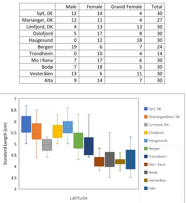
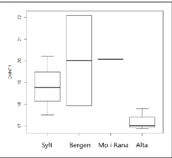
Results from the fieldwork sampling found that stickleback body size (measured as standard length) decreased as latitude increased, in opposition to Bergmann’s rule of species increasing in size toward the poles. Additionally, there was evidence for slight sexual dimorphism in which males were significantly smaller than females across all populations. Furthermore, gravid females were found to be significantly larger than non-gravid females. Results from the target gene qPCR testing found Sirtuin2 to be more expressed in female gonads of northern populations than in southern populations. This is in line with Sirtuin´s role in cold acclimation which would be more beneficial to northern than southern populations. Male gonads showed higher expression of DNMTs and TETs, possibly indicating greater plasticity of epigenetic actors capable of change. This thesis project is the first to study epigenetic differences in fish populations across a latitudinal gradient. Future research could benefit from increasing the
ii
sample size (number of individuals and populations) and/or investigating alternative organs that may also show differential gene expression of epigenetic actors.
Overall, epigenetic mechanisms are likely to be differentially expressed depending on factors of organ, sex, population, and local environmental factors, all of which can potentially allow greater adaptive potential under climate change.
Keywords: Epigenetics, Threespine Stickleback, Gene expression, Latitudinal variation
Resumo
__________________________________________________________
O stickleback de três espinhos é um peixe teleósteo encontrado circunglobalmente e é uma espécie modelo em ecologia evolutiva, pois é conhecido por se adaptar em poucas gerações em relação a outras espécies de peixes. Um dos mecanismos usados para se adaptar a ambientes em mudança é através da plasticidade fenotípica por mecanismos epigenéticos. A adição de um grupo metilo à citosina é conhecida como metilação do ADN, e tem o potencial de causar mudanças rápidas em resposta a estímulos ambientais, tais como mudanças na temperatura ou salinidade. A metilação pode ser transmitida aos descendentes, dando a este mecanismo o potencial para produzir mudanças em toda a população de gerações sucessivas. A metilação pode ser criada por metiltransferases de DNA como DNMT1 e DNMT3ab, e removida por proteínas de translocação Ten-eleven como TET1 e TET3. A aclimatação a frio é a capacidade de um organismo de se adaptar a baixas temperaturas, uma característica particularmente útil na sobrevivência em altas latitudes, caracterizadas por temperaturas de água mais baixas. Os genes potencialmente envolvidos na aclimatação a frio incluem MacroH2A e Sirtuin2 que, além desta função, desempenham outras como a modificação da histona e o metabolismo regulador. A aclimatação térmica e a capacidade de um organismo de regular a temperatura é interessante porque cenários futuros de mudança climática prevêem aquecimento, e a capacidade de um organismo para se adaptar a esta mudança pode determinar a sobrevivência de uma população. Para estudar o papel potencial dos mecanismos epigenéticos na adaptação local das populações de três espinhos de stickleback, foi realizado um trabalho de campo para recolher amostras de tecido de stickleback em 11 locais diferentes ao longo das costas do Mar do Norte e
iii
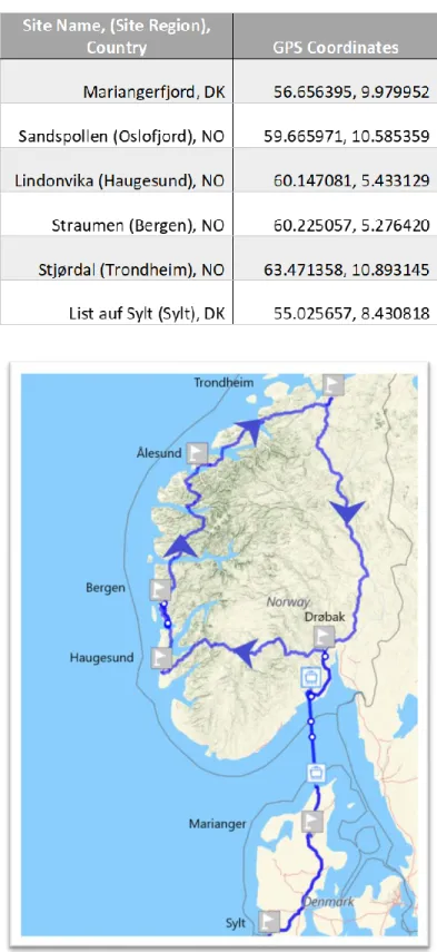
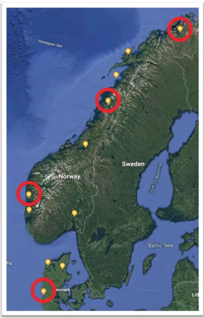
da Noruega. A primeira metade do trabalho de campo foi um "loop sul" que ocorreu entre 6 e 28 de Maio de 2019, partindo e regressando ao Instituto Alfred Wegener em List auf Sylt, Alemanha. A rota seguida foi, sucessivamente: de List auf Sylt, Alemanha para Marianger, Dinamarca; Oslofjord, Haugesund, Bergen, Ålesund, Trondheim, Noruega; e finalmente de volta para List auf Sylt, Alemanha. O Stickleback foi capturado com sucesso por rede de cerco em Oslofjord, Haugesund, Bergen e Trondheim na Noruega, por armadilhas do tipo covo em Mariangerfjord, Dinamarca, e por puça em List auf Sylt, Alemanha. A segunda metade do trabalho de campo foi o "loop norte" que ocorreu entre 3 e 20 de junho de 2019, saindo e retornando da Universidade Nord em Bodø, Noruega. A rota geral seguida foi: de Bodø para Vesterålen, Tromsø, Alta, Mo i Rana (NO), e de volta para Bodø. O Stickleback foi capturado com sucesso por armadilhas do tipo covo em Bodø e Vesterålen, e por puça em Alta e Mo i Rana. Por último, foi feita uma curta viagem até Limfjord, Dinamarca, para amostragem de uma população de stickleback com rede de cerco. Finalmente, 305 indivíduos foram capturados, em 11 populações separadas, com cerca de 30 indivíduos capturados em cada local. O stickleback mostrou ser abundante no Atlântico nordeste e apenas dois dos locais, Ålesund e Tromsø, não computaram stickleback. Os resultados da amostragem de stickleback apresentaram uma tendência de diminuição do comprimento padrão com o aumento da latitude. Esta situação é contrária à regra de Bergmann, que afirma que os organismos aumentam de tamanho em altas latitudes. A tendência encontrada pode ser devido a uma variedade de fatores, como regimes térmicos, luz solar, disponibilidade de nutrientes e complexidade do ecossistema. O comprimento do dorso do stickleback diferiu por sexo e mostrou dimorfismo sexual, com os machos sendo consistentemente mais curtos que as fêmeas. Além disso, as fêmeas portadoras de ovos eram maiores do que as fêmeas sem ninhadas desenvolvidas.
O comprimento padrão do stickleback de três espinhos foi medido, fotografado e foram dissecados gônadas, músculo peitoral, pele, cérebro e brânquias. O dorso do stickleback foi classificado por gênero somente após a identificação visual de suas gônadas. O stickleback feminino foi designado "gravid female" se seus ovários contivessem óvulos totalmente desenvolvidos e esses óvulos fossem segurados frouxamente ou livremente suspensos na cavidade corporal. Todas as dissecações seguiram o procedimento idêntico de eutanásia por
iv
corte preciso da medula espinhal, e amostras de órgãos foram colocadas em tubos Eppendorf contendo RNAlater, rotulados, armazenados em uma criobox, e levados de volta ao Alfred Wegener Institute. No laboratório, as amostras de gônadas e tecido muscular peitoral tiveram o seu RNA extraído utilizando um kit de ADN/RNA da Qiagen® AllPrep™ e as extrações foram normalizadas para conter pelo menos 10 nanogramas por microlitro de RNA. Onze populações tiveram amostras de tecido recuperadas, mas apenas quatro locais foram selecionados para serem usados na análise de expressão gênica para este estudo. Sylt (DE), Bergen, Mo i Rana, e Alta, (NO) foram selecionados porque representavam o comprimento total do gradiente latitudinal desde o Mar do Norte até o extremo norte do Oceano Atlântico. Isso foi feito para aumentar a probabilidade de detecção de diferenças de expressão gênica usando populações o mais afastadas possível.
v
Index
__________________________________________________________
Abstract………i Resumo………ii Index……….v Index of Figures………..………….vi Index of Tables………..……….…….ixAbbreviations, acronyms, symbols……….……….…………x
1 - Introduction………1
1.1 - Climate Change and the Future of Stickleback………..1
1.2 - Marine and Freshwater Stickleback Ecotypes……….……..3
1.3 Genetic Adaptations……….6
1.3.1 - Lateral Plate Adaptations………..6
1.3.2 - Pelvic Girdle and Spine Adaptations……….…….8
1.4 - Threespine Stickleback Biogeography………9
1.5 - The North Sea and Norwegian Sea: Past, Present, and Future………..11
1.6 - Epigenetic Mechanisms of Stickleback Divergence……….14
1.7 - Temperature and Stickleback……….………18
1.8 - Epigenetic Actors Potentially Influencing Thermal Adaptation………..………22
1.8.1 DNMT………..………..22
1.8.2 TET………23
1.8.3 MacroH2A………23
1.8.4 Sirtuin………..…..24
2 - Materials and Methods……….……….25
2.1 - Field Sampling in Germany, Denmark, and Norway………25
2.1.1 - Dissection of Samples……….………32
2.1.2 - RNA Extraction……….……35
2.2 - Gene Expression assays using Quantitative Real Time PCR………..35
2.2.1 - Housekeeping Gene Validation Tests……….……….36
2.2.2 - Target Genes Validation Tests………..38
2.2.3 - qPCR of Target Genes……….39
2.2.4 - Data analysis………....41
3 - Results……….42
3.1 - Field sampling of Temperate to Arctic Stickleback Populations……….42
3.2 - Sea surface temperature and stickleback body size across a latitudinal gradient……...47
3.3 - Target Gene Expression………....49
3.3.1 - DNMT1……….50 3.3.2 - DNMT3ab………52 3.3.3 - TET1……….55 3.3.4 - TET3……….58 3.3.5 - MacroH2A……….…….61 3.3.6 - Sirt2……….…63 4 – Discussion……….66
vi
4.1 Stickleback Populations Across a Latitudinal Gradient………67
4.2 Sex-specific and Site-specific Expression of Epigenetic Genes……….……….69
5 – Conclusion……….73
6 – Acknowledgments………..75
7 – References………..…….75
8 – Annex………86
8.1 Housekeeping Gene Expression………86
8.2 Target Genes Site by Sex Plot ………...89
8.3 Target Gene Sequences………..96
Index of Figures
__________________________________________________________
Figure 2.1. Map of the route of the “southern loop” of the stickleback sampling fieldwork. Figure 2.2. Map of the route of the “northern loop” of the stickleback sampling fieldwork. Figure 2.3. Location of the captured Sylt stickleback population.
Figure 2.4. Location of the captured Bergen stickleback population. Figure 2.5. Location of the captured Mo i Rana stickleback population. Figure 2.6. Location of the captured Alta stickleback population.
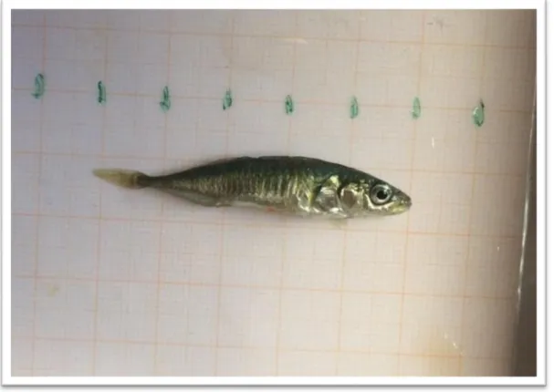
Figure 2.7. An image of a threespine stickleback immediately before dissection. Figure 2.8. The cuts required for stickleback tissue dissection.
Figure 2.9. The V-shaped cuts required for dissecting the brain.
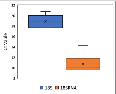
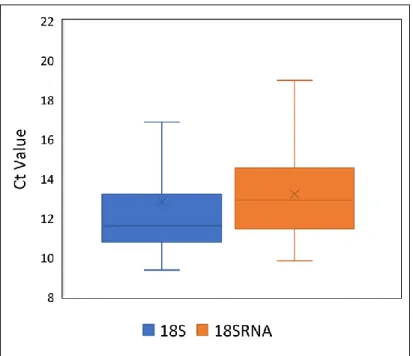
Figure 2.10. Box plot of median (and range) of Ct values for 18S and 18SRNA housekeeping gene validation tests prior to the experiment.
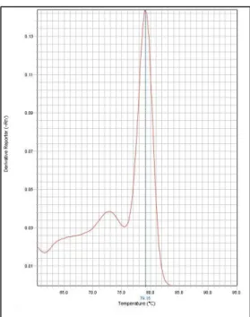
Figure 2.11. Example of a good melting curve showing that DNMT1_1 passed validation. Figure 2.12. Example of a good amplification curve showing that DNMT1_1 passed validation. Figure 3.1. Map of all threespine stickleback locations sampled.
Figure 3.2. The average February and August 2019 ocean temperatures at each sampled location.
Figure 3.3. Box plot of median standard length (and range) of all stickleback populations sampled in order of ascending latitude.
Figure 3.4. Mean standard length ( SD) of stickleback compared between sexes using 9 sampling sites arranged with ascending latitude.
Figure 3.5. Average Ct values of 18S and 18SRNA housekeeping genes obtained during the experiment. Figure 3.6. Box plot of median (and range) DNMT1 expression in both female and gravid female gonads for each of the four sampled populations.
Figure 3.7. Box plot of median (and range) DNMT1 expression of male pectoral muscle averaged for each of the four sampled populations.
Figure 3.8. Box plot of median (and range) DNMT1 expression of pectoral muscle tissue averaged from all sampled populations for each of the three sexes.
vii
Figure 3.9. Box plot of median (and range) DNMT3ab expression of gonad tissue averaged from the three sexes averaged for each the four sampled populations.
Figure 3.10. Box plot of median (and range) DNMT3ab expression of pectoral muscle tissue averaged from each of the three sexes and for each the four sampled populations.
Figure 3.11. Box plot of median (and range) DNMT3ab expression of male pectoral muscle for each of the four sampled populations.
Figure 3.12. Box plot of median (and range) TET1 expression of gonad tissue averaged from each of the three sexes for each the four sampled populations.
Figure 3.13. Box plot of median (and range) TET1 expression of gravid female gonads averaged for each of the four sampled populations.
Figure 3.14. Box plot of median (and range) TET1 expression of pectoral muscle tissue averaged from the three sexes and for each the four sampled populations.
Figure 3.15. Box plot of median (and range) TET1 expression of female pectoral muscle tissue averaged for each of the four sampled populations.
Figure 3.16. Box plot of median (and range) TET1 expression of male pectoral muscle tissue averaged for each of the four sampled populations.
Figure 3.17. Box plot of median (and range) TET3 expression of female gonads averaged for each of the four sampled populations.
Figure 3.18. Box plot of median (and range) TET3 expression of gravid female gonads averaged for each of the four sampled populations.
Figure 3.19. Box plot of median (and range) TET3 expression of pectoral muscle tissue averaged for all sexes for each of the four sampled populations.
Figure 3.20. Box plot of median (and range) TET3 expression of pectoral muscle tissue averaged from each of the three sexes for each the four sampled populations.
Figure 3.21. Box plot of median (and range) TET3 expression of female pectoral muscle averaged for each of the four sampled populations.
Figure 3.22. Box plot of median (and range) MacroH2A expression of gonads averaged from the four sampled populations for each of the three sexes.
Figure 3.23. Box plot of median (and range) MacroH2A expression of pectoral muscle tissue averaged from the four sampled populations for each of the three sexes.
Figure 3.24. Box plot of median (and range) Sirt2 expression of gonads from all sites for each of the three sexes.
Figure 3.25. Box plot of median (and range) Sirt2 expression of female gonads averaged for each the four sampled populations. Populations are ordered on the x-axis with increasing latitude.
Figure 3.26. Box plot of median (and range) Sirt2 expression of pectoral muscle tissue averaged from all four sampled populations for each of the three sexes.
Figure 3.27. Box plot of median (and range) Sirt2 expression of pectoral muscle tissue averaged from all sexes for each of the four sampled populations.
Figure 8.1. Box plot of median (and range) 18S expression averaged over gonads for all sexes across the four sampled populations.
Figure 8.2. Box plot of median (and range) 18S expression in gonads for all sampled populations between the three sexes.
viii
Figure 8.3. Box plot of median (and range) 18SRNA expression averaged over pectoral muscle for all sexes across the four sampled populations.
Figure 8.4. Box plot of median (and range) 18SRNA expression in pectoral muscle tissue for all sampled populations between the three sexes.
Figure 8.5. Box plot of median (and range) DNMT1 expression averaged over gonads for all sexes for each of the four sampled populations.
Figure 8.6. Box plot of median (and range) DNMT1 expression averaged over pectoral muscle for all sexes for each of the four sampled populations.
Figure 8.7. Box plot of median (and range) DNMT3ab expression averaged over gonads for all sexes for each of the four sampled populations.
Figure 8.8. Box plot of median (and range) DNMT3ab expression averaged over pectoral muscle for all sexes for each of the four sampled populations.
Figure 8.9. Box plot of median (and range) TET1 expression averaged over gonads for all sexes for each of the four sampled populations.
Figure 8.10. Box plot of median (and range) TET1 expression averaged over pectoral muscle for all sexes for each of the four sampled populations.
Figure 8.11. Box plot of median (and range) TET3 expression averaged over gonads for all sexes for each of the four sampled populations.
Figure 8.12. Box plot of median (and range) TET3 expression averaged over pectoral muscle for all sexes for each of the four sampled populations.
Figure 8.13. Box plot of median (and range) MacroH2A expression averaged over gonads for all sexes for each of the four sampled populations.
Figure 8.14. Box plot of median (and range) MacroH2A expression averaged over pectoral muscle for all sexes for each of the four sampled populations.
Figure 8.15. Box plot of median (and range) Sirt2 expression averaged over gonads for all sexes for each of the four sampled populations.
Index of Tables
__________________________________________________________
Table 2.1. Site and GPS coordinates of the “southern loop” fieldwork. Table 2.2. Site and GPS coordinates of the “northern loop” fieldwork. Table 2.3. Results of validation tests for 8 candidate housekeeping genes.
Table 2.4. Standard curve efficiencies of candidate target genes during the validation tests. Table 3.1. Sampling site locations ordered by capture date.
Table 3.2. Water temperature data of sampled locations.
Table 3.3. Number of stickleback of each sex category caught at each sampling site.
Table 3.4. ANOVA results for standard length of threespine stickleback populations testing the effects of site and three sex categories.
ix
Table 3.5. ANOVA results for expression of DNMT1 in gonad and pectoral muscle tissue across four threespine stickleback populations and three sex categories.
Table 3.6. ANOVA results for expression of DNMT3ab in gonad and pectoral muscle tissue across four threespine stickleback populations and three sex categories.
Table 3.7. ANOVA results for expression of TET1 gonad and pectoral muscle tissue across four threespine stickleback populations and three sex categories.
Table 3.8. ANOVA results for expression of TET3 gonad and pectoral muscle tissue across four threespine stickleback populations and three sex categories.
Table 3.9. ANOVA results for expression of MacroH2A gonad and pectoral muscle tissue across four threespine stickleback populations and three sex categories.
Table 3.10. ANOVA results for expression of Sirt2 gonad and pectoral muscle tissue across four threespine stickleback populations and three sex categories.
Table 8.1. ANOVA results for expression of the housekeeping gene 18S in gonad tissue across four threespine stickleback populations.
Table 8.2. ANOVA results for expression of the housekeeping gene 18S in gonad tissue across three threespine stickleback sexes.
Table 8.3. ANOVA results for expression of the housekeeping gene 18SRNA in pectoral muscle tissue across three threespine stickleback sexes.
Table 8.4. Tukey test contrasts, multiple comparisons of means for expression of the housekeeping gene 18SRNA in pectoral muscle tissue across threespine stickleback sexes
Table 8.5. ANOVA results for expression of the housekeeping gene 18SRNA in pectoral muscle tissue across four threespine stickleback populations
Table 8.6. Target Gene Sequences
Abbreviations, acronyms, symbols
__________________________________________________________
DNMT - DNA methyltransferase TET - Ten-eleven translocation
MacroH2A - Core histone macro-H2A.1 Sirt2 - NAD-dependent deacetylase sirtuin 2 DE – Germany
DK – Denmark NO – Norway
x
ΔCt – the difference of cycle threshold between the target gene and the housekeeping gene
1
1. Introduction
__________________________________________________________
1.1 Climate Change and the Future of Stickleback
Earth’s evolutionary history can be, in part, defined by cycles of climatic warming and cooling. In the present day, excessive carbon dioxide release by humans is creating a global ‘greenhouse effect’ whereby temperatures are rising and species are being impacted. As of 2018, global warming has contributed to approximately a 1.0⁰C increase in global temperatures with the possibility of a 1.5⁰C increase between the years 2030 and 2052 (IPCC 2018 Special Report). Near the poles, temperatures have risen at least 0.6⁰ C over the last thirty years, which is double the average for the rest of the planet (IPCC 2013). Climate change will undoubtedly have cascading effects on the environment, such as melting of polar permafrost which will, in turn, release more carbon dioxide into the atmosphere (Schuur et al., 2015). Other negative outcomes due to climate change are sea levels rising 0.1 meters by 2100, glaciers and the polar ice caps melting, extreme temperature fluctuations, and increased risks of drought or flooding depending on the region (IPCC 2018 Special Report). Without climate change mitigation by humans, species extinctions and ultimately a global loss in biodiversity will occur (Martin et al., 2019). One study by Warren et al. (2013) suggested that 34 ± 7% of animals will lose over 50% of their present-day range by 2080. Indeed, an earlier review predicted that 80% of the 434 species studied will have their range and abundance shift because of the effects of climate change. Using a meta-analysis of 99 species, it was shown that their range-boundaries will shift toward the poles at a rate of 6.1 kilometers per decade (Parmesan and Yohe 2003).
Fish are particularly vulnerable to the effects of climate change because of changes in water quality, such as temperature, salinity, oxygenation, acidity, and nutrient content. Warmer oceans will have higher sea levels, be more acidic and less oxygenated (due to lower solubility of gases in warm water), become more stratified because of less water mixing, and will have lower average salinity due to changes in precipitation patterns, run-off and melting (Frost et al., 2012). These critical parameters will almost certainly affect at least some marine life with local extirpations and extinction events likely throughout the oceans. In one climate scenario model
2
used by the Intergovernmental Panel on Climate Change, a 1.5⁰C increase in ocean temperature will decrease the annual global fish catch by 1.5 million tonnes (IPCC 2018 Special Report). Besides overall increased mortality and lower reproduction rates, fish populations in the Northern hemisphere are predicted to move northward toward the pole in order to persist in their ideal environmental and habitat conditions. Marine fish in general have higher mobility compared to terrestrial species due to a lack of constraints of their movement, but northward range expansion for marine fish will also have its limit. Different fish species will respond to climate change in different ways, but research by Perry et al. (2005) found that marine fish that are capable of shifting their distribution will be those species with a faster life history and a smaller overall body size than non-shifting species.
The Family Gasterosteidae, also known as the sticklebacks, are a family of 16 species most closely related to pipefish and seahorses (Bell 1994). This family contains five genera; Apeltes – the fourspine sticklebacks, Culaea – the brook sticklebacks, Pungitius – the ninespine sticklebacks, Spinachia – the fifteen-spine sticklebacks, and Gasterosteus – the threespine sticklebacks. There are six species within the genus Gasterosteus, with G. aculeatus representing the most commonly known and best studied threespine stickleback species (hereafter referred to simply as stickleback). Stickleback (Gasterosteus aculeatus, Linnaeus 1758) are commonly found in marine and freshwater habitats across Europe, Asia, and North America. The earliest known fossils of threespine stickleback were found in western California, date to about 13 million years ago, and have a morphology closely resembling modern marine and anadromous stickleback (Bell et al., 2009). Today, stickleback grow to an average total length of 5 cm, and typically range between 3 and 8 cm (Fuller et al., 2019). Stickleback have cryptic coloration, appearing with dark brown or green hues above the lateral line, and shining silver on their underside (Fuller et al. 2019). Sexually mature males, however, display red undersides and bright blue eyes (Frischknecht 1993). Stickleback are predated upon by at least 68 species worldwide since they are abundant in a wide range of habitats, and are usually targeted for their small size and comparatively slow swimming speed (Reimchen 1994). Stickleback have two pelvic and three dorsal spines (giving the species its name), and rather than scales, have bony lateral plates along both sides of their torso centered on the lateral line (Walker 1996). Three main lateral plate
3
morphs are recognized (complete, partial and low plated), with the number of lateral plates varying within and among populations and habitats (Song et al., 2010). The amount of defensive plating per population is linked to tradeoffs with mobility to evade predators versus physical defenses to survive an attack (Bergstrom 2002).
Stickleback are one of the most widely used model species in ecology and evolution. Ancestral stickleback populations lived in the Pacific Ocean, spread to the Arctic and then the Atlantic Ocean during the last inter-glacial period (Fang et al., 2018). Throughout their range, ancestral marine populations colonized brackish and freshwater aquatic environments, resulting in one of the best natural experiments to investigate mechanisms of parallel evolution (Rundle
et al., 2000). Stickleback are highly variable in morphology depending on the environment, and
can be classified as separate ecotypes within certain habitats e.g. benthic or limnetic freshwater ecotypes (Willacker et al., 2010). In addition to their abundance in nature, and hence, their suitability for eco-evolutionary studies of wild populations, stickleback are also often used as a model species in laboratory experiments. They are easy to maintain in aquaria, survive well under laboratory conditions, and can be bred without much difficulty. Genetic variation between populations can occur relatively quickly and can be easily recreated in a laboratory setting, with the added benefit of designing specific lineages in which the environment of a family tree can be strictly controlled (Jones et al., 2012b). In 2006, the first whole genome assembly of the threespine stickleback was completed by the Broad Institute of Cambridge, Massachusetts (Jones
et al., 2012). This sequencing effort led to great strides within stickleback research which
continues to the present day. In this way, stickleback are similar to zebrafish (Danio rerio), another important fish model species whose entire genome has also been sequenced (Jones et
al., 2012). In addition, stickleback are a model organism in behavioural ecology, as they show
large variances in mating behavior and varying levels of cooperative behaviors amongst individuals (Huntingford et al. 1994; Millinski et al. 1992).
1.2 Marine and Freshwater Stickleback Ecotypes
After the retreat of glaciers in the northern hemisphere, marine stickleback colonized new habitats including freshwater lakes and rivers. More precisely, oceanic stickleback can either live
4
an entirely marine life or be anadromous, with spawning occurring either in marine or freshwater, respectively (Madsen et al. unpublished data). Marine stickleback will spawn in the shallow nearshore areas of the coasts, whereas the anadromous or migratory type will spawn in the lower parts of freshwater rivers and streams (Mäkinen et al. 2006). Some stickleback populations diverged and adapted to an entirely freshwater existence while other populations remained anadromous. Freshwater stickleback populations typically have a lower number of lateral plates, missing or reduced spines, a smaller body size, and a fewer number of gill rakers in comparison to oceanic forms (Wantanabe et al. 2003). The freshwater ecotype persists in the northern hemisphere because of parallel divergence through the continuous expansion of the core marine population into lakes and rivers (Raeymaekers et al. 2005).
In the Transporter Hypothesis, all freshwater stickleback populations diverged from core, highly genetically differentiated marine stickleback populations (Liu et al. 2016). In northern Europe and western Canada, stickleback populations in freshwater lakes and streams are only as old as the waterbodies themselves, e.g. since the glaciers melted (Reusch et al. 2001). Molecular evidence for freshwater ecotypes being the derived ecotype comes from analyses of their microsatellites and allozymes, which were found to have lower allelic richness than their marine counterparts, which is typical of a derived population (Reusch et al. 2001). Additionally, rare alleles with low frequency in the founding marine populations have a better chance of being positively selected for in a freshwater-divergent population (Liu et al. 2016). In some cases, freshwater stickleback evolved into different allopatric mitochondrial DNA lineages (mtDNA) which occurred after the Pleistocene. For instance, Scandinavian freshwater lineages can be grouped by western, eastern, and southern types, and likely arose from differing colonization routes from different refugium (Mäkinen et al. 2006). Between 9-8 Kya and 4 Kya, freshwater stickleback populations in Greenland and Northern Europe declined, possibly due to the other periods of glaciation. Contrasting results on the origins of different freshwater populations have found some with an origin of multiple marine populations (Raeymaekers et al. 2005), whereas another freshwater group was found to be monophyletic in origin (Reusch et al. 2001). In most cases, marine populations have more microsatellite diversity and less differentiation due to larger population sizes and a higher rate of gene flow than freshwater populations (Mäkinen et
5
al. 2006). The high adaptive potential and durability of stickleback has enabled it to successfully
thrive in all marine and freshwater habitats in and around the Northern hemisphere.
When a marine stickleback enters freshwater, over 25% of its genome can diverge in just 50 years (Nelson et al. 2018). Typically, reduced gene flow and divergent selection should promote local adaptation. But a theory by Samuk et al. (2017) states that when gene flow and divergent selection occur in tandem, this can slow adaptation because of hybridization between the source and colonized populations. This happens due to a breakdown of positive linkage disequilibrium in which locally adapted alleles are tightly genetically linked on the same chromosome or occur in a site of low recombination (Samuk et al. 2017). Additionally, their results suggest that gene flow may cause the usable area of the threespine stickleback’s genome to shrink, which could place a constraint on future adaptation (Samuk et al. 2017). Suppression of the number of genes recombining while a population is diverging can determine the pattern of genetic differentiation and divergence (Nelson et al. 2018). Indeed, Nelson et al. (2018) found a negative association between genetic divergence and recombination rate. This could help preserve freshwater haplotypes during a transition to a marine environment because of reduced recombination rates (Nelson et al., 2018). Additionally, freshwater chromosome sequence diversity was found to be higher than their marine relatives. Nelson et al. (2018) concludes that these genomic patterns reflect the strong population structure of freshwater stickleback which fortifies them against recombination with marine chromosomes. While the freshwater ecotype is better adapted at preserving their individual genetic identity, marine stickleback appear more susceptible to genetic recombination, and can, theoretically, adapt to climate change in novel ways (Nelson et al., 2018).
Gene flow is thought to homogenize most marine populations due to a higher frequency of migrants flowing between adjacent stickleback populations (Caldera and Bolnick 2008). Despite this uniformity, the genetic diversity of intermixing populations will increase over time as the frequency of allele exchange rises and more random mutations are passed on (Caldera and Bolnick 2008). This increased gene flow has also resulted in marine populations becoming the foundational stable genetic lineage from which freshwater populations have diverged (Reusch et
6
population increases because it creates reproductive isolation and a lack of gene flow (Reusch et
al., 2001). Through this model, brackish or estuarine stickleback have higher gene flow than
freshwater populations because they will be closer to an ubiquitous marine population. Freshwater stickleback will only diverge once they are blocked by a barrier to dispersal that leads to reproductive isolation (Kristjánsson 2005). The rate of migration into a freshwater source depends on abiotic factors of the watershed such as the slope of the channel, flow rates, altitude, waterfalls, and man-made obstacles (Caldera and Bolnick 2008). Freshwater ecotypes suffer from the “founder effect”: reduced genetic diversity because the population arose from a genetically limited number of stickleback. This can result in higher inbreeding, more genetic drift, and a higher risk of extirpation than that in marine populations.
1.3 Genetic Adaptations 1.3.1 Lateral Plates
Lateral dermal plates are a defensive adaptation that threespine stickleback developed to resist penetrating attacks, enlarge their body size, and increase the difficulty of being swallowed (Song et al. 2010). These plates are anisotropic, body conforming, porous, and comprised of acellular lamellar bone (Song et al. 2010). An interlocking mechanism links the armored plates to the pelvic girdle and the basal plate of the spines for added protection (Song
et al. 2010). Marine stickleback typically have over 30 plates while freshwater stickleback have
less than 10, including some ecotypes that lack plates completely (Hansson et al. 2016). There are also partial plate morphs, often residing in brackish water, where fish have an intermediary set of between 10 and 30 lateral plates (Hansson et al. 2016). The number of lateral plates is highly heritable in all three morphological variations, and each variation of plate number can arise independently in geographically isolated populations (Loehr et al. 2012). Hypotheses for the reduction in number of plates in freshwater include predator-prey dynamics, swimming agility and buoyancy, changes in osmoregulation, limited nutrient availability, and energy allocation to growth and development rather than to dermal plates (Wiig et al. 2016).
The development of lateral plates is controlled by numerous genes, the most dominant of which is the ectodysplasin A (Eda) gene on chromosome IV (Wiig et al. 2016). This gene
7
encodes a signaling protein which is also central to growth and development of the skeleton, skin, and teeth (O’Brown et al. 2015). Eda is a recessive gene which has been associated with a reduction in total plate counts in homozygous (aa) freshwater populations (Wiig et al. 2016). Homozygous (AA) sticklebacks are commonly found saltwater with full plating, whereas heterozygous fish (Aa) found in brackish water have only partial plating. Research by O’Brown et
al. (2015) found that low-plated freshwater stickleback have a specific T to G base pair change in
the Eda enhancer Wnt. The Wnt gene signals early proliferation and specification of tissues but also affects Eda expression (O’Brown et al. 2015). Results from this study found that the T to G base pair change decreases Wnt responsiveness, decreasing Eda expression, ultimately reducing the number of lateral plates. When Eda was mutated in its coding region, fish had a complete loss of plates and partial loss of fins and teeth (Iida et al. 2014). However, the T to G change has been shown to lower plate count in stickleback without removing plates, fins, or teeth. This suggests that a nucleotide mutation could be one of the only ways genetically to reduce lateral plate number while still preserving the other important functions of the Eda gene (O’Brown et
al. 2015). There is also evidence from other species that Eda is involved in the development of
ectodermal structures such as hair, feathers, teeth, and sweat glands (Zhang et al., 2018). Disruptions to this gene can lead to hair loss, abnormal feathers or teeth, and even the removal of sweat glands (Zhang et al., 2018). Harris et al., (2008) found that the Eda signaling pathway has an ancestral role in growth of the fish skeleton, and that changes in the functions of these genes will also lead to changes in morphology (Harris et al., 2008)
Predator – prey dynamics play a large role in driving the evolutionary changes associated with the loss of lateral plates in freshwater stickleback populations (Reimchen 1994). While spine length can help stickleback avoid predation entirely, the robustness of the dermal plates often allow it to survive the encounter. Research by Marchinko (2009) found that aquatic insect predation on freshwater stickleback resulted in a reduction of armored plates. One reason is that a higher number of lateral plates can reduce fish speed and velocity, thereby making them easier for a predator to catch (Bergstrom 2002). A heavier body will require a higher energy expenditure to move, and predators will usually have more success capturing a fish encumbered by heavy plating. Additionally, it is possible that a predator can indirectly select for lateral plate number
8
when taking advantage of other another trait, such as the length of spines or slower growth rates (Miller et al., 2017). Longer spines in stickleback could be a disadvantage if it allows predatory insects the ability to grab onto the spines. If longer spines are correlated with higher numbers of lateral plates, then predators with grabbing ability could indirectly lower the number of plates (LeRouzic et al., 2011). Total growth of stickleback can be lower if more energy is allocated to developing lateral plates (Marchinko 2009). Slower growth could extend the juvenile phase or stunt maximum growth, increasing the likelihood of an early death from predation. Thus, the degree to which armored plating can benefit stickleback fitness will depend on the heritability of the traits and the selective pressures of the environment (Bergstrom 2002).
1.3.2 Pelvic Girdle and Spine Adaptations
Marine threespine stickleback have a sturdy pelvic girdle made of dermal bone which is connected to two adjacent pelvic spines. The pelvic girdle is used to strengthen the body and to increase size to avoid predation by gape-limited predators (Ostlund-Nilsson et al. 2006). The pelvic spines are set on a hinge which can be raised or lowered depending on the impeding threat level. Through parallel evolution, many freshwater stickleback populations have either reduced their pelvic girdle or completely lost it (Bell et al., 1993). A leading theory suggests that when predation by fish and birds is strong, the pelvic girdle will become more robust and the pelvic spines will lengthen (Marchinko 2009). When stickleback populations are threatened by high predation by insects, the whole apparatus could be reduced or lost (Miller et al. 2017). Pelvic spines can pierce the soft tissue on the mouths of birds and fish, and an enlarged body can aid in preventing oral ingestion. Insect predators avoid swallowing whole fish by grabbing onto the spines and then ingest the fish piece by piece (Chan et al., 2010). Because fish predation is a strong selective factor in the ocean, genes are continuously passed on that support a strong pelvic apparatus in marine stickleback. Predation by insects is not a factor in the oceans as much as in inland lakes and rivers, which is evidence for why pelvic girdle reduction is only found in freshwater stickleback populations (Marchinko 2009). In the “calcium limitation hypothesis” by Klepaker et al. (2013), it is suggested that freshwater stickleback juveniles have a survival benefit when calcium concentrations in the water are low because it enables them to grow and develop faster without the need to produce extra dermal bone. The reduction of pelvic defense elements
9
have been associated with reductions in lateral plate number in some stickleback populations, suggesting that these processes evolved under similar selection pressures (Klepaker et al. 2013)
Genetically, reduction of the pelvic region is controlled by expression of the Pituitary homeobox 1 locus (Pitx1) at the telomeric end of linkage group 7, and has the accompanying Pel enhancer (Chan et al. 2010). This can occur with a single deletion which removes the enhancer and cripples pelvic growth (Chan et al. 2010). Alleles for pelvic reduction arose independently in many populations of stickleback and all have deletions within the same 484 base pair genomic region where the Pel enhancer is located (Klepaker et al. 2013). Many stickleback populations with a modified pelvic region show directional asymmetry with the right side more reduced than the left (Ostlund-Nilsson et al. 2006). This can also be seen in mice with a null mutation on Pitx1, in which their hind legs are reduced on the right side more than the left (Chan et al. 2010). It has been suggested that this effect occurs due to compensation by Pitx2, which has some control over pelvic function, but not to the degree of Pitx1 (Chan et al. (2010). Research by Chan et al. (2010) found Pitx1 to be one of the most flexible regions of the stickleback genome due to its susceptibility to double-stranded DNA breaks and repair through nonhomologous end joining. Evidence for this extreme flexibility is the high prevalence of deletion mutations in the same genomic region across most stickleback with pelvic reduction (Shapiro et al., 2004). Pitx1 and Pel enhancer mutations arose from natural selection to better adapt stickleback to survive local predation, as has been shown in many freshwater populations (Shapiro et al., 2004).
1.4 Threespine Stickleback Biogeography
Comparing stickleback populations from northern Germany to northern Norway offers an interesting model system to study rapid adaptation due to their recent presence in the region. Here, populations along this latitudinal gradient can be dated to roughly 12,000 years ago, coinciding with the last glacial retreat and glacial buildup around the coasts. Although they have only recently expanded into the region studied here, stickleback have a long evolutionary history beginning in the Pacific Ocean and then spreading into the Artic and Atlantic Oceans (Fang et al., 2018). A study of the biogeographical distribution of threespine stickleback found that most ancestral populations resided in the eastern Pacific Ocean from at least 137.7 thousand years ago
10
(Fang et al. 2018). For the marine clades of the Pacific, there are two main subclades: an eastern Pacific lineage on the west coast of North American, and a western Pacific lineage near Japan and the east coast of Russia. The ancestral stickleback populations in the eastern Pacific Ocean began colonizing the western Pacific Ocean between 79.7 to 37.3 thousand years ago (Fang et al. 2018). In Japanese waters, these two sub-lineages have become reproductively incompatible, representing the Japan Sea and Pacific Ocean clades (Ravinet et al. 2014). Research by Ravinet et
al. (2014) also found that freshwater stickleback around Japan were direct descendants of the
Trans-Pacific Clade and not of the Japan Sea clade. This may indicate higher adaptive potential of the Trans-Pacific Clade, which enabled it to colonize the Arctic and Atlantic Ocean areas (Ravinet
et al. 2014). Earth’s last glacial period during the Pleistocene epoch was defined by frigid
temperatures and glaciation throughout most landmasses above 60o N, and included the
formation of a Bering Sea Land Bridge (Stroeven et al. 2016). Stickleback of the Pacific were only able to colonize the Atlantic after the Bering Sea opened between 110 and 11 thousand years ago (Elias et al., 1996). However, there is also evidence for much earlier stickleback colonization of the Atlantic around 2 million years ago based on mtDNA linages (Orti et al. 1994). This ancient population did not gain a foothold in the region, probably due to population bottlenecks or extinction at the end of the late Pleistocene (Orti et al. 1994)
Through analyses of nuclear and mitochondrial genomes, the two major clades of threespine stickleback are the Euro-North American (ENA) and the Trans-North-Pacific clade (TNP) (Lescak et al. 2014). The TNP clade is found only in the Pacific Ocean whereas the ENA clade occurs both in the Atlantic and eastern Pacific Ocean. Pacific populations expanded from 150-100 Kya to 15-14 Kya, and likely had numerous migrations into refugia during glaciation events over their evolutionary history. Research by Lescak et al. (2014) in the Pacific Ocean found that the two clades follow the isolation-by-distance theory: TNP stickleback had fewer mtDNA haplotypes the further they occurred from the coast of Japan. These linages diverged 1.3-0.9 Mya, and all known subclades of saltwater or freshwater threespine stickleback can trace their genetic lineage back to one of these two clades. Their work also found an environmental barrier to dispersal in the Bussol Strait within the Kuril Island chain, in which the ENA haplotype was absent south of the strait. In the Aleutian Islands, Amchitka Pass was another impasse for
11
stickleback in which different subclades formed on opposing sides of the deep-water channel. Lescak et al. (2014) suggest that a lack of Pleistocene glaciation in the western Pacific allowed the TNP clade to spread more rapidly than the ENA clade, which could only colonize the area after the North American glaciers retreated. Nevertheless, there is some overlap of haplotypes where the two clades meet, resulting in admixture (Lescak et al., 2014).
Euro-North American threespine stickleback were found to have two main mtDNA sub-lineages, Greenlandic and Northern European populations. Research by Liu et al. (2016) suggests that similar demographic history between the two stickleback sub-lineages denotes a similar evolutionary history near the rise and decline of Pleistocene glaciers. However, this does not confirm that the two populations originated from the same refugia, only that their environmental conditions were analogous. One difference between regions is that currently Greenland contains both sub-lineages, whereas in northern Europe only the Northern European lineage is present (Liu et al. 2016). The expansion of the Euro-North American clade began 25-20 Kya and coincided with glacial retreat. Recolonization routes into northern Europe are slightly ambiguous because the Greenlandic clade was close, but a lack of the Greenlandic clade in northern Europe suggests that this was not the path taken, perhaps because of a barrier to dispersal in the northeast Atlantic (Liu et al. 2016). Instead, northern expansion from southern or central European refugia remains the leading theory, in part because this would have occurred in parallel to other historical migrations of fish such as the brown trout, bullhead, grayling, and perch at the end of the last glacial maximum (Teacher et al. 2011). Overall, ENA stickleback show a more recent and faster expansion whereas the TNP clade is much older but expanded at a slower rate (Liu et al. 2016).
1.5 The North Sea and Norwegian Sea: Past, Present, and Future
Lasting from 2.588 million years ago to 11,700 years ago, the present-day Arctic Ocean, North Sea, and coasts of Norway were covered by the Eurasian Fennoscandian Ice Sheet (Soulet
et al. 2013). This event, known as the Weichselian Glaciation, reached its peak coverage during
the last glacial maximum about 24,000 years ago (Stroeven et al 2016). In addition to ice cover, glaciation also caused a global drop in sea levels because of the thermal contraction of seawater,
12
storage of water in glaciers, and “glacial isostatic adjustment”; the gravitational potential and modification of the ocean’s surface in response to a fluctuating surface load (Lambert et al. 2013). Most research on the last glacial maximum has concluded that the present-day northern North Sea was covered by the fusion of the British and Fennoscandian Ice Sheets (Carr et al. 2006). Part of the present-day southern North Sea became tundra, whereas the area north of it became “Doggerland”, an ancient land bridge near a glacier which eventually flooded. After the Younger Dryas period of renewed glaciation ended in 12,000 BP, the global climate warmed and the Fennoscandian Ice Sheet dissolved into a fraction of its maximum size (Borzenkova et al., 2015). The southwestern coast of Greenland was ice-free after 10-9.5 Kya and the Jutland Peninsula was clear by 14 Kya (Liu et al. 2016). In the North Sea, the northern glacial bridge was broken, the British and Fennoscandian Ice Sheets separated, the tundra was flooded, and the modern North Sea was formed. In Denmark, this glaciation period left many fjords such as the Marianger Fjord and the large Limfjord, which spans the entire northern Denmark region. In Norway, where glaciation was more intense, today, the majority of the coastal landscape is fjord lands (Farmer and Freeland 1983).
Today, the North Sea has a total surface area of 575,300 km2 and a total volume of 42,294
km3 (Ices 1983). In the North Sea, the coldest waters are typically found in the southern North
Sea, and the warmest waters in the north at the entrance of the Gulf Stream (Perry et al., 2005). The Gulf Stream enters the North Sea from the north as it rounds the coast of the United Kingdom and moves eastward towards northern Germany. A smaller current of Atlantic water enters the southern North Sea via the English Channel. This current is deflected north to Skagerrak, a large water way between northern Denmark and southern Norway (Hordoir et al., 2013). The Norwegian Atlantic Current moves north from the North Sea bringing warm and salty water throughout the Norwegian Sea (Christensen et al., 2018). The Norwegian Coastal Current lies between the Norwegian mainland and the Norwegian Atlantic Current and carries cold, freshwater from the Baltic Sea up along western coast of Norway to the Barents Sea and the Arctic Ocean. These two currents eventually come together which forms the Norwegian Sea, with a total area of 1.1 million km2 and a volume of over 2 million km3 (Ices 2007). The Baltic Sea has
13
al., 2013), and the summer months are typically when the waters along the Norwegian coasts are
the least saline. Reasons for this include wind-based Ekman transport that moves more surface freshwater of the Baltic Sea into the Norwegian current in the summer, as well as the seasonal snow and glacier melt from the Norwegian mainland (Núñez-Riboni and Akimova 2017). Importantly, there is evidence that the average temperature of the Norwegian current has increased by 1⁰C since 1961 (Christensen et al., 2018).
The Gulf Stream is responsible for the massive transport of heat to western Europe, with winter temperatures up to 10⁰C warmer than similar latitudes in Russia and Canada (Palter 2015). The Gulf Steam plays a vital role in the hydrology of the North Sea and Norwegian Sea by bringing warm surface water from the equator up into the northern temperate region (Palter 2015). In addition to temperature transport, the Gulf Stream also brings saltier water north which mixes with the fresher northern waters that are fed by glacial and ice melt of the Arctic ocean (Rhines
et al., 2008). One of the most pressing outcomes of climate change is the weakening of the Gulf
Stream and possible changes to the thermohalinity composition in this region. Stenevik and Sundby (2007) suggests with a medium confidence of 33-67%, that the global balance of temperature and salinity will weaken because of a warming climate. A weaker Gulf Stream current will bring a reduced amount of warm water to the North and Norwegian Seas, which will lower temperatures and could decrease the salinity of the oceans. Artic sea ice melting and glaciers melting in Norway and Greenland will likely add a large volume of freshwater into the Arctic ocean, which would be prevented from mixing if the reduction of thermohaline cycling creates a less turbulent ocean (Polyakov et al., 2010). Additionally, there are effects of “albedo” creating a positive feedback loop which could speed up warming in this region. Albedo is the reflection of solar energy back to the atmosphere when coming into contact with reflective ice (Perovich et al., 2007). If enough surface ice were to melt, then more solar radiation will be absorbed by the Earth and increase climate warming (Palter 2015). The extent of these effects on the temperature of the North Sea and Norwegian Sea are currently not known and difficult to determine because at least some of the temperature changes will offset each other. For example, there will be a cooling effect from a weakened Gulf Stream but a warming effect from anthropogenic causes and reduced albedo effects (Perovich et al., 2007).
14
Increasing water temperatures will lead to decreases in the amount of dissolved oxygen in the water, leading to expansive hypotonic regions in the oceans. This is, in part, could drive the northward movement of aquatic species in which organisms seek more habitable and oxygenated conditions towards the poles (Shaffer et al., 2009). In theory, the most northern populations are at the highest risk of extinction under climate change scenarios because there is less new space to migrate to in the north. Populations in the southern range are also at risk of extirpation due to living on the periphery of their optimal conditions and extremes warm temperatures (Shaffer et al., 2009). However, southern populations and species will usually have a wide area north in which to shift their range, increasing their likelihood of survival in the long-term. In warmer waters, fish will suffer from oxygen-limited stress as dissolved oxygen decreases. These restrictions limit functions that require aerobic activity such as overall growth, swimming ability, and reproduction (Portner and Knust 2007). For example, Pacific salmon can be blocked from migrating upriver when the water temperature is too high due to higher aerobic costs imposed on them (Farrell et al., 2008). If these higher temperatures are combined with greater difficulty in reaching spawning grounds, reproduction may be impossible, as was the case in 2004 for the Weaver Creek Sockeye population (Farrell et al., 2008).
1.6 Epigenetic Mechanisms of Stickleback Divergence
Ecological epigenetics is an expanding research field due to the potential for epigenetic modifications to lead to faster phenotypic variation that genetic change (Giuliani et al., 2015). With genetic change, an organism’s genotype and phenotypes are modified slowly over time due to changes in the underlying DNA sequence being shaped by natural and sexual selection. While DNA sequence change occurs more slowly, it maintains a high degree of stability and is more resistant to change, whereas epigenetic modifications happen faster but are more unstable and liable to change (Richards et al., 2010). Epigenetic modifications can regulate gene expression without modifying the underlying DNA sequence (Metzger and Schulte 2017). Epigenetic responses initiate chemical or structural modifications in chromatin, histone protein complexes, and sites of DNA spooling (Deichmann 2016). With genetic change, the specific order of cytosine, guanine, adenine, and thymine nucleotides are affected, and this can only occur across successive generations. Epigenetic change, however, can work much faster though effects such as
15
methylation of cytosines, which does not affect the underlying nucleotide structure and can occur solely based on environment stimuli (Giuliani et al., 2015). Potentially thousands of CpG methylation events can occur in just 30 generations, which is typically much faster than genetic evolution (Johannes and Schmitz 2018). This rate of methylation is not only affected by the rate of new methylation events, but also resistance to demethylation (Graaf et al., 2015). If environmental conditions remain stable for a long enough time, it is possible that epigenetic changes could lead to genetic evolution over time (Graaf et al., 2015).
The most commonly studied epigenetic mechanism in wild population is DNA methylation. DNA methylation is the addition of a methyl group onto a cytosine nucleotide causing regulatory changes to gene expression, typically resulting in the repression of a gene (Metzger and Schulte 2018). This involves a covalent modification of cytosine that is copied during cell division at 5'-cytosine-phosphate-guanine-3' sites (CpG) by the enzyme DNA methyltransferase I (Feinberg and Fallin 2015). The vertebrate genome contains many CpG sites and heritable methylation can only occur at these dinucleotide sequences (Schübeler 2015). While contiguous regions of methylated CpG can affect gene expression, it is also possible that a single methylation can influence the regulation of a gene (Smith et al. 2015). This methylation is functionally involved in the repression of genetic traits, X chromosome inactivation, and the silencing of repetitive DNA (Jones 2012). DNA methylation also plays a role in differentiation of pluripotent cells, such as diverging somatic cells from stem cells (Feinberg and Fallin 2015), and methylation in the centromere is important in maintaining chromosomal stability (Jones 2012). Bisulfite (HSO3-) treatments are used on DNA to replace unmethylated cytosines with uracil while
leaving the 5-methylcytosine intact (Schübeler 2015). Afterwards, polymerase chain reactions (PCR) are used to amplify this sequence which enables mapping of the methylated DNA even to a single base resolution (Olova et al. 2018). This analysis can be completed with dead cells, a limited amount of DNA, or on low quality DNA unlike more sensitive RNA or protein analyses (Schübeler 2015).
Besides DNA methylation, other epigenetic mechanisms include post-translational modifications of nucleosome proteins, and varying densities of nucleosomes and chromatin within the nucleus (Feinberg and Fallin 2015). The occurrence of an epigenetic modification is
16
reliant on a combination of environmental influences and existing genetic structure. Indeed, Johannes and Schmitz (2018) postulate that the malleability of the epigenome being resistant to spontaneous methylation is genetically based. Phenotypic plasticity is the ability of an organism’s genome to respond to varying environmental signals (Pigliucci et al., 2006). Developmental plasticity is a type of phenotypic plasticity that can occur in early development when exposed to an environmental stimulus such as changing temperature or salinity, and can cause lifelong changes in the organism (Hanson et al., 2011; Bateson et al., 2004). This mechanism can give the organism an early benefit to thrive in its immediate environment, but can be negative if the environmental factors it adjusted to are in flux (Hanson et al., 2011). Another type of plasticity, known as phenotypic flexibility, occurs when epigenetic-induced changes to gene expression result in temporary acclimation that is reversible depending on the organism’s current environment (Metzger and Schulte 2018). This type of epigenetic acclimation is more ‘loosely’ held by the organism and can be continually adjusted throughout the life of the organism. However, the degree of benefit the organism receives is less than with developmental plasticity (Hanson et al., 2011; Metzger and Schulte 2018). Epigenetic modifications have the potential to shape future generations of an organism if the addition of a methyl group can persist through cell division, potentially leading to genetic diversification of a population and possible divergence (Metzger and Schulte 2017). This mechanism occurs because DNA methylation can maintain stability throughout meiotic cell division (gametogenesis) and embryogenesis (Fellous et al., 2018), allowing future cell divisions with the retained epigenetic factor. This effect is plastic because epigenetic-induced DNA methylation can undergo reprogramming and methylation loss in two occurrences, the germline phase and in the initial embryo phase (Fellous et al., 2018). This loss allows for the placement of new occurrences of methylation to be responsive to the environment and allows epigenetic modification to occur once again.
Latitudinal variation of epigenetic diversity within populations is a novel research field because climate change scenarios predict poleward movement of many species, especially marine fishes (Perry 2005). Water temperature typically decreases toward the poles, since the warmer waters of the equator receive the most direct sunlight and the poles the least. Tolerance of water temperatures is driven in large part by genetic differences between populations of a
17
single species (Pereira et al., 2017). However, there is evidence that average ambient temperatures are also playing a role in thermal tolerance, which could be driven by epigenetic factors (Pereira et al., 2017). As a recently developing field, ecological epigenetic research in wild populations is limited in general, and focused analyses of the potential relationship between epigenetic variation and latitude are even more scarce. Difficulties in studying the correlation between these two factors stems from the need to research a single species that is spread over a large enough area to potentially show epigenetic differences between subpopulations. One species that has been studied in this context is Norwegian Spruce, a boreal confer inhabiting northern Europe. A study by Yakovlev et al., (2010) investigated the ‘epigenetic memory’ of this spruce in different regions by studying miRNA sequence length. They found that Norwegian Spruce’s embryos are affected by ambient temperature at the time of development, which effects the development of its bud (Yakovlev et al., 2010). In follow up research, Yakovlev et al. (2014) showed that temperature conditions during zygotic and somatic embryogenesis significantly changed transcriptional profiles in genetically identical Norwegian spruce trees. They proposed that the underlying mechanism may be a type of “multi-positional thermal switch” that can activate or silence certain gene pathways during embryogenesis based on ambient temperature (Yakovlev et al., 2014). While it is currently unknown how an epigenetic “thermal switch” would work, modifications of histone structure, in similar ways to that of DNA methylation, could be a likely candidate (Li et al., 2005; Yakovlev et al., 2014).
Threespine stickleback distribution and abundance has been shaped by its ability to acclimate to a range of temperatures throughout the northern hemisphere (Bell 1994). The retreat of Pleistocene glaciers enabled stickleback to colonize further north and into colder waters, and their ability to respond to selective pressures via phenotypic plasticity has played a large role in shaping short and long-term adaptations (Foster et al., 2003). Fish are ectotherms whose internal body temperatures are regulated by the temperature of their environment. Genomic DNA methylation variation is hypothesized to be the product of temperature affecting the rate of deamination of methylated cytosine, known as the “methylation-temperature-deamination-hypothesis” (Metzger and Schulte 2017). Higher body temperatures are related to reduced guanine-cytosine content because elevated temperatures increase the mutation rate of
18
cytosine to thymine, thus increasing the rate of deamination (Metzger and Schulte 2017). Amongst different species of fish, previous research has found higher genomic DNA methylation in polar fish compared to equatorial fish (Varriale and Bernardi 2006). For stickleback, research by Metzger and Schulte (2017) found higher occurrences of DNA methylation when stickleback were exposed to increased temperature during early juvenile development and adult acclimation. While the increase in methylation found could result from the methylation-temperature-deamination-hypothesis, it is also a possibility that the raised temperature caused a change in cellular phenotype, such as the proportion of oxidative and glycolytic muscle fibers (Metzger and Schulte 2017). Further research by Metzger and Schulte (2018) found that regulation of muscle growth can vary in response to varying temperature treatments, and this plays an important role in thermal plasticity of fitness-related traits. If these epigenetic changes can be inherited by offspring, this could increase the fitness of stickleback populations in the face of rapid climate change (Metzger and Schulte 2018). For example, Shama et al., (2016) found that expression of genes involved in mitochondrial respiration in F2 generation offspring were differentially regulated depending on the thermal environment that their mother and grandmother experienced, suggesting an underlying epigenetic mechanism of inheritance.
1.7 Temperature and Stickleback
Water temperature is a critical environmental parameter which affects fish growth, reproduction, immune response, oxidative capacity, distribution, rate of metabolism, rate of digestion, and behavior (Dietrich et al., 2018; Long et al., 2013). A fish species´ ability to adapt to temperature can play a major role in its distribution, as this abiotic parameter can create a natural barrier to dispersal. Beitinger et al., (2000) suggest that sudden changes in ambient water temperature are a major cause of large-scale fish kills due to internal surpassing of thermal minimums and maximums. Adaption to temperature requires acclimation to not only a mean optimal temperature but also to fluctuations caused by time of day, weather, ocean currents, and seasonal differences (Huey and Bennett 1990). Diurnal fluctuations in temperature can restrict growth if the mean temperature is above the optimal temperature (e.g. too hot), and when ambient temperature is below optimal, e.g. too cold (Jobling 1997). Stochastically fluctuating environments, however, have been shown to increase growth (Shama 2017), likely