Continuous evaluation of the stiffness of stabilized soils since compaction: enhancements to the EMM-ARM methodology

Luís Miguel Rios Vieira

Continuous evaluation of the stiffness of

stabilized soils since compaction:

enhancements to the EMM-ARM methodology

Luís Miguel Rios Vieira

November 2014 UMinho | 201 4 Continuous e valuation of t he s tif fness of s

tabilized soils since

com paction: enhancements to t he EMM-ARM me thodology

Escola de Engenharia

November 2014

Master’s Thesis

Integrated Ms Civil Engineering

Work performed under the supervision of

Professor António Gomes Correia

And co-supervision of

Professor Miguel Azenha

Luís Miguel Rios Vieira

Continuous evaluation of the stiffness of

stabilized soils since compaction:

enhancements to the EMM-ARM methodology

Escola de Engenharia

i

Acknowledgments

I would like to thank to all persons who made this dissertation possible namely:

- Professor António Gomes Correia, supervisor of this dissertation, for his advices and for sharing his knowledge and experience.

- Professor Miguel Azenha, co-supervisor of this dissertation, for his enthusiasm, motivation and help especially in the writing process;

- PhD student Jacinto Silva for his patient, motivation and availability throughout this entire work;

- all technicians in the Civil Engineering Laboratory at University of Minho for their help during the experimental programs particularly to Mr. José Gonçalves;

iii

Abstract

The stabilization of soils has been used for the improvement of its characteristics to meet required performances. Binders are widely used for the stabilization process, and thereby the soil suffers a hardening process during which its mechanical properties are improved, namely its stiffness. Monitoring the stiffness evolution over the hardening time can reveal important information for quality control, and early identification of potential problems. The EMM-ARM (Elasticity Modulus Measurement through Ambient Response Method) has been applied to stabilized soils in pursuit of a robust method that actually allows continuous measurement of the stiffness of a stabilized soil since very early ages. EMM-ARM is based on the identification of the resonance frequency of a composite beam that comprises the tested material, over the curing time and allows inferring the E-modulus of the stabilized time through the dynamic equation of motion of the beam.

This technique has been used on stabilized soils with success. However, the technique still lacked a sampling method that allowed retrieving representative samples from in-situ layers. This dissertation aimed to contribute for the development of the EMM-ARM technique namely in developing a sampling procedure that can be applied on practical conditions. Therefore, a specific sampler was developed for EMM-ARM, and its feasibility has been proved through an experimental program for validation.

Moreover a new EMM-ARM variant that allows direct in-situ tests was proposed in order to avoid the uncertainties related with the sampling process. This variant consists on the identification of the resonance frequency of a steel bar that is partially embedded in the tested layer of stabilized soil. Even though the pilot applications revealed sensitive issues of the proposed technique, its viability and feasibility has potential to be further improved.

Key Words

v

Resumo

A estabilização de solos tem sido usada para o melhoramento das suas características para o cumprimento de requisitos de desempenho. Os ligantes são amplamente utilizados para o processo de estabilização, e desse modo o solo sofre um processo de endurecimento durante o qual as suas propriedades mecânicas são melhoradas nomeadamente a sua rigidez. A monitorização da evolução da rigidez ao longo do período de endurecimento pode revelar informações importantes para o controlo da qualidade e para a identificação de potenciais problemas. A técnica EMM-ARM (Elasticity Modulus Measurement through Ambient Response Method) tem sido aplicado a solos estabilizados de forma a encontrar um método que realmente permita a medição contínua da rigidez de solos estabilizados desde as primeiras idades. O EMM-ARM é baseado na identificação da frequência de ressonância de uma viga mista que inclui o material a testar, ao longo do período de cura e permite deduzir o módulo de elasticidade no tempo de estabilização através de equações de equilíbrio dinâmico.

Esta técnica tem sido usada com sucesso em solos estabilizados. Contudo a técnica ainda não possui um método de amostragem que permita a recolha de amostras representativas de camadas estabilizadas in-situ. Esta dissertação tem o propósito de contribuir para o desenvolvimento da técnica EMM-ARM nomeadamente em desenvolver um processo de amostragem que possa ser aplicado em condições reais de campo. Neste contexto, foi desenvolvido um amostrador específico para o EMM-ARM, e a sua viabilidade foi comprovada através da execução de um programa experimental.

Além disso foi proposto uma nova variante do EMM-ARM que permite ensaios in-situ de forma a evitar as incertezas relacionadas com a amostragem. Esta nova modalidade de ensaio consiste em identificar a frequência de ressonância de uma viga de aço parcialmente embebida numa camada de solo estabilizado. Apesar da aplicação piloto ter revelado alguns problemas de sensibilidade da técnica proposta, a sua potencialidade merece aperfeiçoamento futuro.

Palavras-chave

vii

Table of Contents

1

INTRODUCTION ... 1

1.1 General remarks ... 1

1.2 Dissertation Structure ... 3

2

EXPERIMENTAL ASSESSMENT OF THE ELASTICITY MODULUS

IN STABILIZED SOILS ... 4

2.1 Laboratory tests ... 4

2.1.1 EMM-ARM ... 4

2.1.2 Uniaxial compression test ... 11

2.1.3 Bender elements ... 12

2.1.4 Ultrasonic tests ... 13

2.2 Field tests ... 15

2.2.1 Static load plate test ... 15

2.2.2 Light Weight Deflectometer ... 16

2.2.3 Humbolt stiffness gauge ... 17

2.3 E-modulus vs strain level ... 18

2.4 Overall summary table ... 20

3

DEVELOPMENT OF SAMPLER ... 21

3.1 Sampling: general considerations ... 21

3.2 Block sampling ... 21

3.3 Tube Samplers ... 23

3.3.1 Design considerations ... 23

3.3.2 Drive samplers ... 26

3.3.3 Rotary Samplers ... 31

3.4 Sample driving techniques ... 32

3.5 Summary of sampler types ... 35

viii

3.7 Proposed sampler and driving technique ... 38

4

EXPERIMENTAL PROGRAM ... 43

4.1 Materials and mixture proportions ... 43

4.1.1 Soil ... 43

4.1.2 Cement ... 45

4.1.3 Mixture proportions ... 45

4.2 Pilot application ... 46

4.2.1 Overall Strategy ... 46

4.2.2 Preparation of the mixture and placement ... 47

4.2.3 Sampling ... 48

4.2.4 Description of the test procedures for E evaluation ... 49

4.2.5 Results ... 51

5

PROPOSAL OF A VARIANT OF EMM-ARM ... 55

5.1 Concept ... 55

5.2 Proposed pilot model ... 57

5.2.1 Performance requirements ... 57

5.2.2 Preliminary numerical studies ... 58

5.2.3 Detailed simulations of the proposed setup ... 59

5.3 Pilot experiments ... 62

5.3.1 Experimental setup ... 62

5.3.2 Strategy and procedures... 63

5.3.3 Results ... 66

5.3.4 Evaluation in view of numerical simulations ... 67

6

Conclusion ... 71

6.1 General conclusions ... 71

6.2 Future Developments ... 72

ix

List of Figures

Figure 1 - Resonant frequency identification process over testing time (Silva et al. 2013)

adapted ... 5

Figure 2 - Comparison between compression tests(blue) and EMM-ARM technique (Azenha 2009) ... 6

Figure 3 - U-shaped cross section (Silva 2010) ... 7

Figure 4 - Tubular PVC mould: (a) cross-section; (b) lateral view (units: mm) (Silva et al. 2013) ... 8

Figure 5 - The windows of Hanning with 50% overlap ... 9

Figure 6 - Average of the FFT segments ... 10

Figure 7 - Sketch of half-beam ... 11

Figure 8 - Uniaxial compression test with LVDTs mounted (Silva 2010) ... 12

Figure 9 - Sketch of a Bender elements setup after(Alvarado & Coop 2012) ... 13

Figure 10 - Schematic Ultrasonic setup (Yesiller et al. 2001) ... 15

Figure 11 - Load Cell and Plate Set Up from NCDOT ... 16

Figure 12 - Light Weight Deflectometer (Adam & Adam 2003) ... 17

Figure 13 - Humbolt equipment ... 18

Figure 14 - Steps of the Simpson model compared with the real stiffness-strain curve (Benz 2007) ... 19

Figure 15 - Moduli as a function of strain level for various numerical simulations and test analysis ... 19

Figure 16 - Schematic diagram of the Sherbrooke down-hole block sampler (Lefebvre & Poulin 1979) ... 22

Figure 17 - Dimensions of a tube sampler (Clayton et al. 1998) ... 23

Figure 18 - Influence of AR in sample quality (Siddique et al. 2006) ... 24

Figure 19 - Analytical solutions for axial strain history at the center-line of the sampler for different B/t ratio (Clayton et al. 1998) ... 25

Figure 20 - Shelby tube available at the University of Minho ... 27

Figure 21 - Scheme of theU100 sampler (Bell 2004) ... 28

Figure 22 - SPT Sampler ... 28

x

Figure 24 - Osterberg hydraulic piston sampler (Osterberg 1973) ... 31

Figure 25 - a) Single tube corebarrel (Murthy 2002) b) Denison triple-tube corebarrel (Johnson 1940) ... 32

Figure 26 - X-ray photographs of sampling by hammering (left) and pushed (right) (Briaud 2013) ... 34

Figure 27 - Slide hammer (Hmtri 1997) ... 34

Figure 28 - Prismatic mould: a) Lateral view; b) cross-section; c) scheme of the set sampler / mould (Silva et al. 2014) ... 36

Figure 29 - Phases of the sampling process with the prismatic mould (Silva et al. 2014) .. 37

Figure 30 - Details of the sampling with the PVC tube (Costa 2011) ... 38

Figure 31 - Dimensions of the sampler (mm)... 39

Figure 32 - Sampler and detail of the cutting edge... 40

Figure 33 - Preliminary test ... 41

Figure 34 - Driving procedure ... 42

Figure 35 - Granulometric curve of the sand ... 44

Figure 36 - Compaction curve of the Sand ... 45

Figure 37 - Compaction curve of the Sand-Cement mixture... 46

Figure 38 - Overall Strategy ... 47

Figure 39 - Preparation of the UCC Specimen adapted from (Magalhães 2013) ... 48

Figure 40 - Apparatus of the sampling ... 49

Figure 41 - EMM-ARM test ... 50

Figure 42 - a) accelerometer b) signal acquisition system (Costa 2011)... 50

Figure 43 - UCC setup ... 51

Figure 44 - Load-Displacement curve for the sampler ... 52

Figure 45 - EMM-ARM results ... 53

Figure 46 - UCC stress-strain relationship ... 53

Figure 47 - EMM-ARM vs UCC test results ... 54

Figure 48 - Scheme of the concept ... 56

Figure 49 - Schematic showing transducer and specimen well connected to charge amplifier, frequency response analyser and personal computer (Meredith 1999) ... 57

Figure 50 - Sketch of the proposed model (dimensions in mm) and 3d view from Multiphysics ... 59

xi

Figure 52 - Computed relationship between the resonant frequency of the embedded steel

bar and the E-modulus of the tested material ... 61

Figure 53 - Derivative of the frequency ... 61

Figure 54 - Beam used and sharped edge ... 63

Figure 55 - PVC container ... 63

Figure 56 - a) PVC tube with the wooden pestle b) Plastic sheet involving the container . 64 Figure 57 - Scheme of the guide (dimension in mm) ... 65

Figure 58 - Beam with the guide ... 65

Figure 59 - Setup in a preliminary test ... 66

Figure 60 - Results in frequency domain ... 66

Figure 61 - Results of the new technique compared with the results of the previous chapter ... 67

Figure 62 - Results of B1 with an elasticity modulus of 205 GPa and 210 GPa ... 68

Figure 63 - Results of the bar 2 for a 15,3-15,4cm length of the cantilever ... 69

Figure 64 - Results of the bar 3 for a 15,3-15,4cm length of the cantilever ... 69

List of Tables

Table 2 - Combinations of AR and OCE ... 26

Table 3 - Hvorslev's driving methods as in (Nagaraj 1993) ... 33

Table 4 - Summary of the samplers ... 35

Table 5 - Grain size of the sand ... 43

Table 6 - UCC specimens results ... 54

Table 7 - The three first modes ... 62

Glossary

EMM-ARM (Elasticity Modulus Measurement through Ambient Response Method) AR Ratio of area

BE Bender Element

xii

E Elasticity Modulus ELFWD Strain Modulus

Ev2 Strain Modulus

ESSG Soil Strain Modulus

FFT Fast Fourier Transform G Shear Modulus

H1 Internal height along the cutting edge

H2 External height along the cutting edge

I Inertia

ICA Inside cutting angle ICR Inside clearance ratio ltt Distance tip-to-tip

LVDT Linear Variable Differential Transformer LWD Light Weight Deflectometer

M Constrained Modulus OCA Outside cutting angle OCE Overall cutting edge PVC Polyvinyl chloride R External Radius

R1 Radius at the bottom edge of the sampler

R2 Radius along the sampler

t Tickness

tt Travel Time

UCC Unconfined compression cyclic tests

VEM-STIFF Very Early age Material Stiffness Monitoring Vp P Wave Velocity

Vs Shear Wave Velocity

n Poisson‟s ratio

w First Flexural Resonance Frequency α External cutting angle

1

1 INTRODUCTION

1.1 General remarks

The behavior of a foundation soil is decisive for the performance of civil engineering structures. Frequently soil characteristics fail to meet the necessary performance requirements to ensure structural safety. In such cases, the soil may be replaced by a better performing material. However, this can be quite impractical and expensive. Therefore, a frequently adopted alternative consists in improving the existing soil properties through a process that is known as stabilization. The stabilization of soils may be achieved by its mechanical compaction or through the addition of chemical additives such as cement or lime. Soil stabilization may improve several properties, such as the soil swelling potential, permeability, shearing and compressive strength (Anifowose 1989; Bell 1993). The use of cement or lime to improve the geotechnical characteristics of soils has become widely used because it allows customized control of the properties of the material through the proportions of the mixture, while being quite feasible from the economic point of view (Horpibulsuk et al. 2006; Quigley 2006).

According to Quigley (2006) the traditional stabilization process through chemical additions includes four main stages:

 lime or cement uniformly spread by mechanical means;  mixing and pulverization of the soil;

 trim and lightly compact followed by mellowing for a period of time;  heavy compaction to ensure air voids of 5% or less.

The geotechnical behavior of treated soils depends on its chemical and physical properties, that are directly related with the soil formation conditions and mineralogical composition (Kennedy et al. 1987).

Lime stabilization is more suitable for soils with high content of clay while cement can be used in any soil with the exception of highly organic soils or some highly plastic clays (Bell 1993; Amu et al. 2011).

2

As concluded by Nagaraj et al. (2014) the combination of cement and lime can be mutual beneficial in some cases as in earth blocks because cement stabilizes the sand portion of the soil whereas lime stabilizes the clay portion.

The chemical stabilization techniques have been used in pavements base layers, slope protection, channel linings, to prevent liquefaction and as a base layer to shallow foundations ( Bell 1993;Consoli et al. 2011; Portelinha et al. 2012).

The ratio binder-soil needs to be determined in laboratory tests in order to control the performance of the mixture in achieving the target proprieties in terms of stiffness, strength and durability. This experimentally based determination of mix proportions is necessary because there are no general methodologies established on rational criteria for the prediction of the mechanical proprieties based on the mixture (Viana da Fonseca et al. 2009).

According to Consoli et al. (2011), dosage methodologies and soil-cement strength have been most conveniently assessed by unconfined compression tests. This technique allows the assessment of the small-strain stiffness of the tested material. However its use at early ages is limited due to the lack of strength of the material that induces relevant experimental difficulties in handling and loading.

Other techniques have been used for the measurement of the small-strain stiffness namely techniques based on wave propagation such as the bender elements (Ferreira 2009) or the ultrasonic tests (Yesiller et al. 2001). These techniques allow non-destructive tests without affecting the properties of the material although these techniques have some uncertainties on the interpretation of results.

A new technique called EMM-ARM has been proposed in 2009 (Azenha 2009) to continuously and automatically measure the stiffness of concrete and cement paste since the fresh state (i.e. right after casting). More recent research works have shown the feasibility of application of EMM-ARM on testing the stiffness of stabilized soils (Silva 2010). This methodology allows overcoming the main limitation of the unconfined compression tests of its use at early ages. Moreover it allows the continuous monitoring instead of discrete instants of time. Compared with the benders and ultrasonic the results of the EMM-ARM technique do not have the uncertainties associated with the wave propagation techniques.

3

Despite de success of EMM-ARM applications to stabilized soils it requires the specimen to be reconstituted in the mould in order to perform the test. However recent applications (Silva et al. 2014) included a preliminary sampling process that proved the feasibility of sampling on EMM-ARM but without the required robustness.

This dissertation has the purpose of contributing for the development of the EMM-ARM technique, particularly in concern to the sampling procedure. The dissertation also outlines an initial attempt for a variant to EMM-ARM that allows direct in-situ testing of a stabilized soil without needing to extract samples (VEM-STIFF technique).

1.2 Dissertation Structure

Besides the present introduction, Chapter 2 provides a literature review of methods for assessment of the elasticity modulus with special emphasis to the EMM-ARM technique.

In Chapter 3 a new sampler and sampling technique are proposed for the EMM-ARM methodology. This chapter includes a literature review of existing samplers and previous attempts of EMM-ARM application that included sampling.

Chapter 4 concerns the practical application of the developed sampler, within the scope of a validation experimental program.

A new variant of the EMM-ARM technique is proposed in Chapter 5, where a set of pilot experiments are presented.

The dissertation is closed by an outline of its main conclusions and prospected further developments (Chapter 6).

4

2 EXPERIMENTAL

ASSESSMENT

OF

THE

ELASTICITY

MODULUS IN STABILIZED SOILS

2.1 Laboratory tests

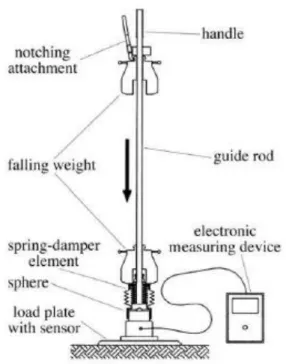
2.1.1 EMM-ARM

2.1.1.1 Concept

EMM-ARM (Elasticity Modulus Measurement through Ambient Response Method) is a technique that allows the continuous measurement of the elasticity modulus of hardening materials (e.g. cement-based materials) since early ages. In its original implementation (Azenha 2009), this methodology consisted in successively identifying the first flexural resonance frequency of a simply supported composite beam composed by an external mould which is internally filled with the material to test (concrete). The technique assumes that the ambient vibration is sufficient to excite the beam for the output-only modal

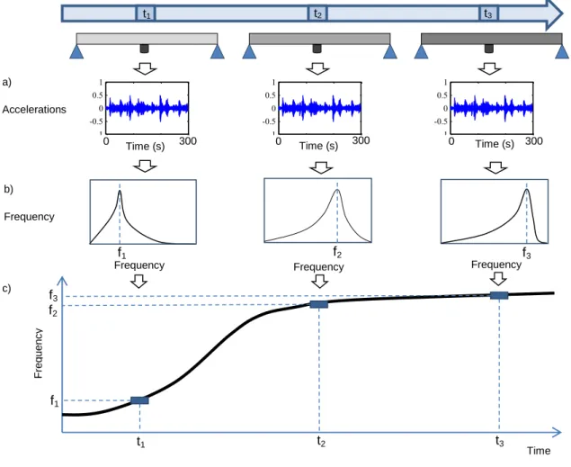
identification. As can be seen in Figure 1 the identification of the resonance frequency is repeated over the time through the measurement of the accelerations (a), which are converted into the frequency-domain (b). It is then possible to obtain a frequency-time curve of the beam (c).

5

Figure 1 - Resonant frequency identification process over testing time (Silva et al. 2013) adapted

The identified resonant frequency is then correlated with the elasticity modulus of the tested material through application of the dynamic equation of motion of the simply supported beam (Silva et al. 2013). It is therefore possible to convert the frequency-time curve into the desired elasticity modulus-time curve.

2.1.1.2 Developments in EMM-ARM since its creation

The first application of the EMM-ARM technique was performed in concrete (Azenha 2009). The pilot experiment was accomplished through a simply supported 2-meter acrylic tube of 0,1m diameter, filled with concrete, put into simply supported conditions and placed within a controlled temperature and humidity. The material was monitored in the first 28 days with an accelerometer which allowed the identification of the first flexural resonance frequency of the beam in that period. The frequency was then correlated with

0 600 1200 18001800 -1 -0.5 0 0.5 1 Time (s) Frequency a) Accelerations 0 600 1200 18001800 -1 -0.5 0 0.5 1 Time (s) 0 600 1200 18001800 -1 -0.5 0 0.5 1 Time (s) Time (s) 300 300 300 0 0 0 Frequency Frequency b) Frequency Fr e q u e n c y Time c) Time (s) Time (s) t1 t2 t3 f1 f2 f3 t1 t2 t3 f1 f2 f3

6

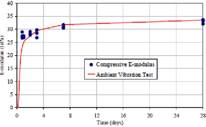
the elasticity modulus. To validate the EMM-ARM results, cyclic compressive tests were performed in cylinders for comparative purposes. The Figure 2 shows the results:

Figure 2 - Comparison between compression tests(blue) and EMM-ARM technique (Azenha 2009)

As can be seen in Figure 2 the compressive tests corroborated the feasibility of EMM-ARM. Following the success of the application in concrete, the technique was then successfully tested in cement pastes (Azenha 2009).

The application of the technique to stabilized soils was then tested by Silva (2010). As the sand-cement materials have a lower elasticity modulus than concrete it was necessary to adapt the technique to these materials thus the mould was redesigned to ensure that the range of resonant frequencies during the experiment was large enough to allow the proper identification of stiffness evolution (Silva et al. 2013). The new mould was made of polycarbonate and had a U-shaped cross-section with an inner size of 40mm x 40mm, as shown in Figure 3 and a span of 495mm. This mould also had the interesting particularity of being reusable.

7

Figure 3 - U-shaped cross section (Silva 2010)

Even though the pilot experiments were considered successful, Silva et al. (2013) reported some important drawbacks: (i) due to the low slenderness of the mould, the frequencies are much higher than in previous applications in concrete, making the specimen less excitable and thus making modal identification more difficult; (ii) the material to be tested needs to be compacted directly into the mould which may complicate the replication of in-situ conditions in terms of compaction level.

Silva (2010) has overcome the above-mentioned limitations with a new design for the mould. The new mould is a 50 mm-diameter PVC tube with 3mm thickness and 1000mm span. This new mould has the capability of being used for in situ sampling as the tube can be directly inserted into the soil as used in recent works (Silva et al. 2014; Costa 2011) to directly recover samples. Moreover the PVC is a cheaper and more adaptable solution than the former acrylic U-shaped mould. Since then, the tube has been undergoing small modifications as a slightly reduction of the span and thickness. The mould has been tested with samples directly retrieved from a layer and with reconstituted specimens where the bulk density is controlled.

The applications of EMM-ARM technique to sand-cement materials have been successful, providedthat the characteristics of the specimens as the bulk density or the content of the mixture are representative of the soil to test. For example a difference of 100Kg/m3 can result in a difference of 0.5 GPa as in previous works (Silva et al. 2014).

Despite the success in the existing application of EMM-ARM to stabilized soils, there are some issues associated that still need to be addressed to improve the applicability of this methodology:

8

 Deviations of ambient vibration from white noise conditions, with strong contamination at certain frequency levels are a recurrent problem that brings added difficulties to the identification of the resonance frequency.

 EMM-ARM still lacks a sampling procedure that can be used on in-situ conditions. Indeed, the development of a sampler that allows the retrieving samples that represent the in-situ conditions is of utmost importance.

2.1.1.3 Procedure/methodology applied to stabilized soils

The latest procedure of EMM-ARM (Silva et al. 2013) consists in placing the freshly mixed material in a PVC tube (50mm of outside diameter and 1.5mm tick), as presented in Figure 4. The PVC tube has known geometry, mechanical properties and support conditions (normally a simply supported tube (Silva et al. 2013; Costa 2011). The mould can be filled whether by sampling or by placing the fresh mix into the mould by hand (here termed as „reconstitution‟).

For a reconstituted specimen the mixture is placed inside the mould with the bottom side sealed. The soil-cement is progressively compacted in the mould with a steel rammer and the density is controlled by weighing the sample, as to achieve a target density value corresponding to in-situ conditions after compaction (Silva et al. 2014). For a sampled specimen the compaction is made directly on the layer and then retrieved for the mould. Either way, after being adequately filled, the mould is sealed in both extremities with wooden disks (Silva et al. 2014). Screws are used to assist the materialization of simply supported conditions near the extremity of the mould, as shown in Figure 4.

Figure 4 - Tubular PVC mould: (a) cross-section; (b) lateral view (units: mm) (Silva et al. 2013)

An accelerometer is attached at the bottom mid-span surface of the mould and connected to an acquisition system. The accelerometer will measure the accelerations suffered by the beam over a defined time (e.g. sets of 300 acquired at intervals of 900s).

9

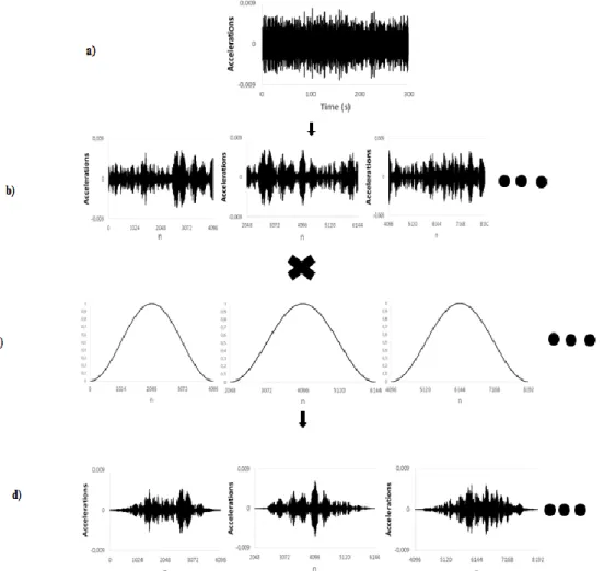
The data is then treated using the Fast Fourier transform (FFT) following the Welch procedure (Welch 1967), thus converting data from time-domain to frequency-domain, on sets that usually comprise 2048 or 4096 points. The data processing is schematically shown in Figure 5, starting with the initial data (a) of 300s split up in overlapping segments (an overlap of 50% is used in EMM-ARM) (b). Each segment has 4096 points for a total of 73 segments are then multiplied by Hanning windows (c).

Figure 5 - The windows of Hanning with 50% overlap

The Fast Fourier Transform (FFT) is applied to each of the segments mentioned above after windowing (d), thus converting the data into the frequency domain. The Welch procedure ends by averaging of the frequency spectra obtained from all segments. A typical result can be observed in Figure 6.

10

Figure 6 - Average of the FFT segments

With the spectrum in the frequency-domain, the next step is to identify the resonance frequency. The Peak Picking method, which is straightforward and robust is used for such purpose. This method is based on the assumption that for frequencies close to the resonance frequency of the structure, the dynamic response is essentially conditioned for the contribution of the resonance mode for example in Figure 6 the frequency in which the structure had more response/intensity was at 51,15 Hz (Magalhães 2012).

Following the identification of the resonance frequency it is necessary to correlate the frequency to the E-modulus of the tested material through the equation of motion. Azenha (2009) presented an equation that relates the first flexural resonance frequency (w) with the stiffness of a simply supported beam ( ̅̅̅) with a concentrated mass at the mid-span (mp)

and length (L) for the case that the supports are flexible, as at the time it was not possible to assure the rigidity of the supports. Meanwhile through new experimental procedures it was possible to assure the rigidity of the supports thus the deduced equation for infinite rigidity of the supports is:

( ) ( ) ( ) ( ) ( ) ( ) (1) Where:

√̅

̅̅̅ (2)

11

Figure 7 - Sketch of half-beam

Upon knowledge of ( ̅̅̅), and based on the fact that the stiffness and inertia of the mould/specimen are known, it is possible to directly infer the E-modulus of the tested material with the following equation.

̅̅̅= EmouldImould + Etesting materialItesting material (3)

The process is repeated for every set at every age of the material in order to obtain the continuous curve E modulus-time.

2.1.2 Uniaxial compression test

The uniaxial compression test consists in applying a compression stress on the longitudinal axis of a specimen and then measures the strains normally in the range of very small to small strains. The stress is applied at a controlled speed, at each instant the stress applied and the strains locally measured by each transducer on the specimen are registered (Gomes Correia et al. 2006). This technique allows the performance of non-destructive tests through cycles of load and unload in which the specimen is submitted to loads in the elastic limit of the material. The Figure 8 presents a uniaxial compression test using a load cell and with LVDTs measuring the displacement.

12

Figure 8 - Uniaxial compression test with LVDTs mounted (Silva 2010)

The measurement of the strains requires equipment of high precision, the most common are the LVDTs (linear variable differential transformer) and the LDT‟s (local deformation transducer).

2.1.3 Bender elements

Bender Elements (BE) have many benefits that make them a desirable technology on the use on tests regarding the determination of material properties. This technique is a non-destructive way of dynamic testing on soils and can measure the stiffness parameters at a specific stress level without apply stresses or deform the specimen in order to perform the measurements. Also, it is possibly to change the frequency at which the BE is excited in order to better accommodate the material being tested and to obtain the clearest signal possible. It has multi-directional capabilities and can be incorporated in many setups - including triaxial and resonant-column tests, presenting smaller strain levels and remaining entirely in the elastic region (Marjanovic 2012) .

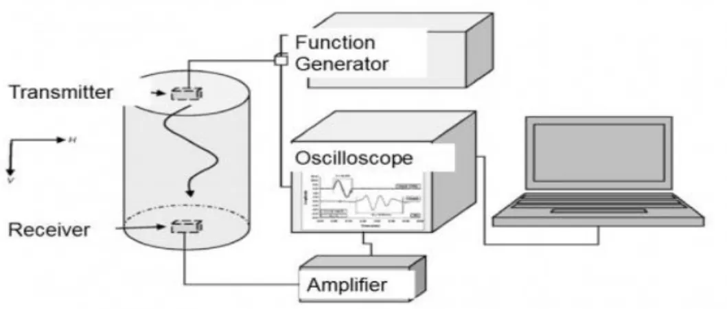
Shirley and Hampton (1978) were the first to measure shear wave velocity (VS) using bender elements. Figure 9 presents a typical schematic diagram of bender element system. Basically the system comprises of two bonded thin piezoelectric plates, which are usually coated with epoxy resin. Two such elements (transmitter and receiver) are normally placed opposite one another and the BE cantilever inserted at a small distance into the soil sample. The transmitter element distorts or bends when subjected to the voltage signal from the function generator and creates the shear waves. The shear wave travels through the specimen and causes the receiver element to vibrate and the arrival time of signal is recorded by an oscilloscope. The interval between the times of transmitted and received signal is calculated as the travel time (tt) of the shear wave. VS is then calculated by

13

dividing the distance travelled by the shear wave over the tt taken. The shear wave travel distance is normally considered as the distance between tip-to-tip (Ltt) of BE (Brignoli et

al. 1996). The shear modulus is calculated through:

(4)

Where is the mass density of the medium and Vs is the velocity of the waves.

Figure 9 - Sketch of a Bender elements setup after(Alvarado & Coop 2012)

Despite allowing non-destructive tests and being a relatively cheap test there are some uncertainties on reading the results namely the distance and time of propagation of the wave.

2.1.4 Ultrasonic tests

The tests through the transmission of supersonic waves are based on the theory that the speed of propagation of waves through the medium depends on the elastic properties and the density of the medium (Meyers & Chawla 2008). Thus, this technic may be used to ascertain the mechanical and physical properties of soils (Stephenson 1978) or cementitious materials (Voigt et al. 2006). The advantage of the technique is to be a non-destructive method. This method can use compression waves (P) and/or shear waves. The wave travels through the specimen and as in benders elements the arrival time is recorded. The interval between the times of transmitted and received signal is calculated as the travel time (tt) of the wave. VS/VP is then calculated by dividing the distance travelled by the

14

ascertain the dynamic module of deformability and the Poisson‟s ratio through the following equations: ( ) (5) ( ) (6)

To determine the elasticity modulus it is required to know the velocity of the two waves and as the sensors only work with one type of wave the application of the technique can become complex. Due to the transdutors characteristics it is more efficient to use P waves, using just this wave, it is possible to obtain the constrained modulus M and the dynamic modulus E if the Poisson ratio is known.

(7)

( )( ) ( )

(8)

The application of the technique can be performed using probes, the test is easy and fast although the interpretation of the results namely identifying the exact time of the wave propagation can be problematic. The sensibility of the operator in the interpretation of the data is a matter of the utmost importance for the precision of the results. The Figure 10 shows a schematic representation of ultrasonic test setup (Yesiller et al. 2001).

15

Figure 10 - Schematic Ultrasonic setup (Yesiller et al. 2001)

2.2 Field tests

2.2.1 Static load plate test

The Static load test plate is a technic that allows the determination of the characteristics of deformability of the layers. It is a laborious and time-consuming technique, whereby normally the number of trial is limited, not providing a statistical basis about the quality of layers (Gomes Correia et al. 2009). There are several testing standards, for instance AFNOR NF P94-117-1. This test has a purpose of ascertain the module of deformability under static load applied to a plate on a platform.

The test is based on the application, after a preload, of two successive cycles of loading through a plate of stiffness and diameter standardized. In the first load cycle, during the time required to stabilize the displacement of the plate it should be maintained an average stress on the plate of 0,25 MP. During the second load cycle the average stress on the plate should be 0,20 MPa and, as in the first period, the unload should be performed only after stabilization of deflection. The strain modulus, Ev2, is calculated for the second load period

by the Boussinesq solution, using the secant method according to the equation for rigid plates (Gomes Correia et al. 2009):

( )

16

Where  is the Poisson ratio, p is the pressure on the plate, r is the radius and z2 is the

displacement of the plate.

In Figure 11 is a set up by the North Carolina Department Of Transportation.

Figure 11 - Load Cell and Plate Set Up from NCDOT

2.2.2 Light Weight Deflectometer

The Light Weight Deflectometer or LWD is a portable equipment to determine, “in situ”, the dynamic modulus of deformation (E). The principle of working is based on the fall of a mass from a defined height over a rigid circular loading plate. The impulse to inflict load is measured through a load cell and the displacement through geophones After measuring the displacement of the plate and the charge applied it is possible to determine the strain modulus ELFWD, through Boussinesq solution (Gomes Correia et al. 2009) using the

following equation:

( ) (10)

In which k is equal to π /2 or 2, to rigid or flexible plates, respectively, δc is the

displacement on the center of the plate, σ is the tension applied and R is the radius of the plate. The Figure 12 shows the equipment normally used in this test.

17

Figure 12 - Light Weight Deflectometer (Adam & Adam 2003)

2.2.3 Humbolt stiffness gauge

Humboldt Stiffness Gauge also called as “geogauge” is an equipment, used “in situ” that through non-destructive testing allows the determination of the stiffness of the layer and the modulus of deformability (E). The geogauge, as presented in Figure 13, can be used in different materials as soils or treated soils. This equipment has a rigid ring that contacts the soil and an electromechanical vibrator that produces frequencies in the range between 100Hz and 196 Hz, with increments of 4 Hz, generating 25 specific frequencies and forces of about 9N. This vibration force produces small deflections that are measured by the geogauge. A microprocessor calculates the stiffness (k) for each frequency and presents the average value. The stiffness can then be converted into soil strain modulus (ESSG) by the

equation (Gomes Correia et al. 2009):

( )

(11)

Where k is the stiffness presented by the geogauge, the Poisson ratio and R the radius of the rigid ring.

18

Each test takes about 75 seconds and according to the National Cooperative Highway Research Program the results will have high variability when testing non-cohesive, well-graded sands or similar soils and the modulus readings from the gauge represent an equivalent modulus for the upper 25,5 cm to 30,5 cm of the layer. Therefore the gauge should not be used to test thin (less than 101,6cm) or thick (greater than 30,5 cm) layers without proper material calibration adjustments.

Figure 13 - Humbolt equipment

2.3 E-modulus vs strain level

The E value measured by each test is influenced by several parameters such as the strain amplitude during the test, the mean effective stress, the void ratio, the preconsolidation stress or the effective material strength (Houlsby et al. 2005;Benz 2007).

Particularly the strain level that the soil sustains during the E measurement test is highly influential on the elasticity modulus value. The effect of the strain level on the Elasticity modulus value can be simulated through some constitutive models. For instance the Simpson brick model is a widely used model in which a strain level step corresponds to a determined elasticity modulus (Benz 2007). This model gives an approximation of the real stiffness-strain curve as can be seen in the Figure 14.

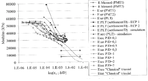
Gomes Correia et al. (2004) through numerical simulations of the Menard pressuremeter test (PMT) and plate load test (PLT) showed the modulus as function of strain level. Figure 15 shows the results.

19

Figure 14 - Steps of the Simpson model compared with the real stiffness-strain curve (Benz 2007)

Figure 15 - Moduli as a function of strain level for various numerical simulations and test analysis

As can be seen in the Figure 15 the numerical tests carried out by Gomes Correia et al. (2004) showed the degradation of the modulus with the increase of the strain on the soil. Moreover the interpretation of the tests was proved as being influential on the results for instance the secant modulus of the unload-reload cycle of the Menard test is around 2.2 times the tangent modulus.(Gomes Correia et al. 2004).

Thereby each e modulus obtained is used in a different manner. When the strain level have a value below 0,5% it is used for deformation analysis for values above it is used for

20

ultimate state analysis such as bearing capacity or stability analysis (Gomes Correia et al. 2004).

2.4 Overall summary table

Table 1 summarizes the presented methods of elasticity modulus assessment:

Table 1 - Assessment tests summary

Test Main measured

parameter Strain Level Remarks

EMM-ARM

E -small strain

stiffness <10

-6 Allows the automatic continuous

measurement since early ages

UCC E -small strain

stiffness <5 x10

-5 Generally used

Limited use at early ages

Benders G0-Small strain

Shear modulus <1x 10

-6 Easy to use but there are some

doubts on reading the results

US

M Constrained modulus E Dynamic Modulus

10-6% Same as benders

SLP Ev2strain modulus 10-3% Time consuming and costly

LWD ELFWD strain modulus

Between 10-3

and 10-4 More portable than the static plate

Humbolt ESSG soil strain modulus

Reported as

small Fast but depth limited

In this dissertation it will be used EMM-ARM and UCC tests. Therefore the parameter assessed will be the small-strain stiffness. For small strains the variation of the modulus is minimal and the values can be directly compared.

21

3 DEVELOPMENT OF SAMPLER

3.1 Sampling: general considerations

In order to directly characterize the soil of a given layer, direct sampling of the soil for laboratory testing can be considered as highly recommended. Samples retrieved from the soil can be grouped in 3 categories: non-representative samples that are unsuitable for laboratory testing, representative samples that contain all mineral constituents of the layer without contamination of other material but might not be representative of the state of water content or micro-structure (Nagaraj 1993) and undisturbed samples that are those which are obtained with the minimum disturbance to the in-situ conditions (Marcuson III & Franklin 1979). The disturbance can occur during drilling, sampling, transportation, storage or preparation for testing. According to Clayton et al. (1995), the mechanisms associated with disturbance can be:

 changes in stress conditions;  mechanical deformation;

 changes in water content and voids ratio:  chemical changes.

To assure that the characteristics of the specimens are representative of those found in the field, collecting undisturbed samples is a matter of the utmost importance. That is especially the case when evaluating the mechanical properties of the soil such as the deformation modulus.

There are several techniques for soil sampling, with the most common being block sampling and tube sampling.

3.2 Block sampling

The method that involves less disturbance, due to the fact that the soil does not suffer shear stress, is the block sampling and is considered the bench-mark (Siddique et al. 2006).

22

A block sample can be retrieved from a pit/exposure by trimming the soil with a sharp knife or retrieved from a borehole using a specific sampler as the Sherbrooke sampler. Excavation of a pit can be an economical way of acquiring a very detailed record of the complex soils conditions although in some conditions such as in normally and lightly overconsolidated clays, the excavation of a pit or shaft with more than a few meters is often impossible (Clayton et al. 1995). The Sherbrooke sampler can overcome that problem because it only requires a borehole of 40 cm diameter. The sampler has a trimming mechanism that cuts the soil. In the Figure 16 is the apparatus proposed by Lefebvre & Poulin (1979) for retrieving block samples.

Figure 16 - Schematic diagram of the Sherbrooke down-hole block sampler (Lefebvre & Poulin 1979)

In this technique the sampler is lowered to the base of the hole using a mechanically-induced or electrically-mechanically-induced rotation. A cylinder of about 250mm in diameter is carved out by 3 circumferential blades at the base (Clayton et al. 1995). Despite allowing high quality samples the process is complex and time-consuming.

23

3.3 Tube Samplers

Tube samplers are driven or rotated into the soil to retrieve a sample. Tube sampling is an easier and less time-consuming way of collecting samples, as compared to block sampling. For such reasons, it is the most widespread technique (Clayton et al. 1995). A tube sampler can be retrieved from pits/exposures or boreholes, and in some cases directly driven or rotated into the soil.

3.3.1 Design considerations

The characteristics of the tube samplers are related to the quality of the sample. Therefore it is important to consider its dimensions in the selection of the tube sampler to further obtain better sampling quality. In the analysis of samplers quality, the block sampling is normally used as the benchmark because such method is known to induce very small levels of disturbance. Figure 17 shows the geometrical data that is used to characterize a tube sampler. In which R is the external radius, R1 is the radius at the bottom edge, R2 the radius

along the sampler, H1/H2 the internal/external height along the cutting edge, α/β the

external/internal cutting angle and t the thickness.

Figure 17 - Dimensions of a tube sampler (Clayton et al. 1998)

The analysis of the expected performance of a given tube sampler can be made through evaluation of geometrical ratios. The most widespread index is the ratio of area (AR) that relates the inside diameter in the cutting edge with the outside diameter (Clayton et al. 1998; Siddique et al. 2006).

24

(12)

As described by Hvorslev (1949) the ratio is a relation between the volume of displaced soil and the volume of the sample itself. To compare the effect of AR on sample quality Siddique et al. (2006) performed tests in Bangladesh clays in which the AR of tube sampler was varied whereas the cutting edges and length were kept constants. Figure 18 presents the results of e(strain), s(shear strength) and E(initial tangent modulus), which were normalized to the corresponding values obtained through the block sampling technique.

Figure 18 - Influence of AR in sample quality (Siddique et al. 2006)

It can be observed that an increase of AR induces an increase of the disturbance of the sample namely an increase of strain and a decrease of shear strength and initial tangent modulus E. The shear strength and the initial modulus in tube sampling is inferior than in block sampling as its value is below 1 regardless the AR. Thus as expected the block sampler gives the best sample. As AR is reduced, so do the changes in stress condition and the mechanical disturbance of the soil structure (Briaud 2013). Siddique (1990) recommends to use an AR of less than 10%.

Another parameter used to evaluate the sample disturbance is the relation external diameter-thickness (R/t) of the sampler. Through numerical analysis, Clayton et al. (1998)

25

were able to estimate the strain caused by sampling along the sampler for different R/t values, as presented in Figure 19 ( in the figure R is named as B):

Figure 19 - Analytical solutions for axial strain history at the center-line of the sampler for different B/t ratio (Clayton et al. 1998)

As can be seen in Figure 19, higher values of R/t correspond better the sample quality. The maximum strain can be obtained by 0,385 t/R, the simplicity and precision of this equation means that can be used in a practical and simple way to estimate disturbances of tube samplers a R/t between 40 and 47 is used in United States practice (Baligh et al. 1987).

Another parameter of importance is the Inside Clearance Ratio that is produced by swaging the cutting edge of the tube, creating a different radius at the bottom edge of the tube (R1)

and at the inside of the tube (R2).

(13)

The ICR reduces the friction between the sample and the inside wall of the tube during sampling (Marcuson III & Franklin 1979) , thus has been introduced in the tube samplers to prevent jamming.

Although it minimizes the shear stresses between the soil and the inside of the tube, it allows lateral expansion of the soil once in the tube, thus the ICR increases the sample

26

disturbance. Clayton et al (1998) recommended an ICR between 0,4% and 1,5% and Kelleher et al.(2008) recommended an ICR inferior to 1% to maximize sample quality.

The design of the cutting edges affects the sample quality. An increase of the outside cutting edge angle (OCA) or the inside cutting edge angle (ICA) means an increase of the strains (Clayton et al. 1995; Siddique 1990).

( ) (14) ( ) (15)

Tanaka (2008) concluded that a small cutting edge angle allows better sample quality than big angles. Siddique (1990) recommended that the samplers should have a small OCA, preferably not more than 5º and an ICA of 1º to 1.5º.

A reduction of the overall cutting edge (OCE) can be used to counter the effects of a high area of ratio (AR) (Clayton et al. 1998). The International Society for Soil Mechanics and Foundation Engineering's Subcommittee on Problems and Practices of Soil Sampling (1965) suggested combinations of AR and OCE for 75mm samplers. The Table 2 shows the proposal combinations.

Table 2 - Combinations of AR and OCE

3.3.2 Drive samplers

Drive samplers are samplers that are pushed or driven into the soil without rotation generally cutting the soil with a sharp cutting edge at their base. The volume of soil corresponding to the thickness of the sampler is moved to the surrounding soil which is either compressed or compacted (Clayton et al. 1995). The characteristics of the sampler depend on the soil to test. Drive samplers can be classified according to their thickness, to the presence of extremity opening (open-drive samplers) or to the inclusion of a piston

27

(Clayton et al. 1995). In this dissertation they are divided in 3 groups: thin-walled (open-drive), thick-walled (open-drive) and piston samplers (thin and thick-walled).

3.3.2.1 Thin-walled drive samplers

The Shelby tube or thin wall tube was introduced in the United States in the 1930´s. It has an AR of 11.7% and a cutting angle of about 44. A further improvement was made in the modified Shelby with an AR of 4.3% and an angle of 5 °(Landon 2007). Their geometrical characteristics induce very low disturbance to the soil. Therefore, these samplers are mainly used with clays and silts and retrieve undisturbed samples suited to many quality laboratory tests (Briaud 2013).This sampler has the disadvantage of being easily damaged. Figure 20 shows the Shelby tube available at the University of Minho.

Figure 20 - Shelby tube available at the University of Minho

3.3.2.2 Thick-walled drive samplers

A thick-walled sampler is a sampler whose AR is greater than 20%. Although is a more expensive sampler than a thin-walled, has more strength and is more suitable for harshest soils. The sample retrieved is usually more disturbed than in thinner samplers.

The British U100 is one of the most common thick-walled samplers. The sampler is driven into the ground through a slide-hammer. Between the sampler and the hammer is a drive head that contains a valve which allows the release of the air while the tube is introduced into the soil and helps to held the sample in place when it is being withdrawn (Bell 2004). Figure 21 presents a scheme of the U100 sampler. Both the drive head and the cutting shoe

28

are screwed to the sampler. The sample retrieved has a nominal radius of 100 mm and a length of 450mm. The AR of the sampler is 27% and the OCA above 20. The value of the area ratio is increased when a liner is used (40%) (Clayton et al. 1995). These values of AR and OCA are very high therefore the expectable sample is of poor quality.

Figure 21 - Scheme of theU100 sampler (Bell 2004)

Split barrel samplers are thick-walled samplers which are divided into two halves lengthwise. During the introduction into the soil these are held together by the shoe and head which are screwed on to each end (Clayton et al. 1995). This allows to easily examine and extract samples from the sampler itself as the soil can be retrieved when the sampler is opened. The sampler used during the SPT (shown in Figure 22) and the modified California sampler are examples of split barrel samplers.

29

This type of sampler has a very high area ratio, it is used primarily with sand and gravels, and it has be acknowledged to collect disturbed samples well suited for soil identification and classification purposes (Briaud 2013).

3.3.2.3 Piston drive samplers

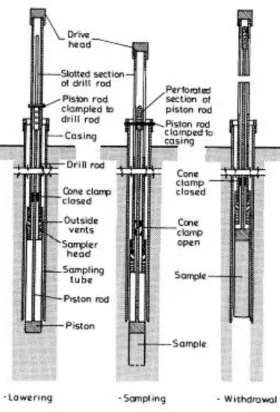
These samplers contrary to the open-drive samplers have the lower end of the tube closed with a piston which can be held stationary, withdrawn or left free to allow flexibility of operation (Nagaraj 1993).

The piston can contribute for a good quality in sampling. Samplers can have a piston in order to: prevent soil of entering in the sampler before the desired collecting position is achieved, to reduce sample losses, to reduce the entry of soil in excess in the tube during the initial stage of driving, to increase the acceptable ratio length / diameter ratios (Clayton

et al. 1995) and to serve as an effective check valve (Nagaraj 1993). The piston can be

used in both thin and thick walled tubes, permitting to obtain high quality samples.

There are several ways of held a piston in a sampler. The Geonor sampler/piston is a widespread solution that comprises a thin walled sampler which uses a stationary piston as presented in Figure 23. In this case the sampler is lowered to the level at which sampling is to start (if a borehole is used), the piston rod is then fixed to the drilling rod and the sampler goes down while the piston stays at the initial position (Clayton et al. 1995) in other words the piston is placed at the bottom of the sampler and stays stationary while the sampler slides down to collect the sample. When the sampler is full the piston and the sampler are pulled.

30

Figure 23 - Sampler with stationary piston (Nagaraj 1993)

This sampler allows to collect undisturbed samples of soft to stiff cohesive soils (Fang 1990). It also allows a good sample quality in loose/media dense sands if the hole is filled with drilling mud (Marcuson III & Franklin 1979).

There are several samplers with stationary piston, such as the Japanese sampler of 75mm with stationary piston, that has an AR of 7.5% allows samples with slightly inferior quality to that obtained by the Sherbrooke sampler (Tanaka 2008).

The Osterberg thin-walled hydraulic piston sampler, presented in Figure 24, has a low AR of 6% and uses two pistons.

The operation mode is similar to the stationary piston as one of the pistons (fixed piston) is held at the starting ground of sampling while the sampler goes down, moreover this sampler has one piston (floating piston) that goes down the tube by hydraulic pressure applied at ground level (Clayton et al. 1995). The sampler cannot be over-pushed since the push stops when the moving piston contacts the fixed piston (Fang 1990).

31

Figure 24 - Osterberg hydraulic piston sampler (Osterberg 1973)

According to Raymond (1977) this sampler is suitable to sensitive clays. Hunt (2005) recommended this sampler for very soft to firm cohesive soils. Marcuson III & Franklin (1979) pointed out that with this sampler it is not possible to limit the sample length.

3.3.3 Rotary Samplers

The rotary drilling uses the rotation combined with a downward force on the material and allows retrieving undisturbed samples of rocks. The rotary samplers can be applied to rocks and soils, but are more easily used in intact rocks than in fractured rocks and soils (Clayton et al. 1995).

The simplest form of a rotary corebarrel consists, as presented in Figure 25a, of a single tube with a coring bit at its lower edge which is loaded and rotated while a pressurized fluid passes around the bit (Clayton et al. 1995). In drive sampling the soil displaced by the walls of the sampler is moved to its vicinities but in the rotary samplers the material is ground up and removed by air, circulating water, or by a drill fluid (Nagaraj 1993). Samples collected with a single tube corebarrel may experience some disturbances due to torsion, swelling or contamination by the drilling fluid (Murthy 2002). The modern corebarrels have two tubes, an outer tube that rotates and an inner tube that remains

32

stationary. Normally the inner tubes are provided with a swivel head that prevents the core from rotating and eroding (Nagaraj 1993).

There are also the barrels of triple tube, as the Denison corebarrel presented in Figure 25b, in which a liner is inserted inside to facilitate the storage of the sample, similarly to the case of drive samplers.

a) b)

Figure 25 - a) Single tube corebarrel (Murthy 2002) b) Denison triple-tube corebarrel (Johnson 1940)

The quality of the samples retrieved by the rotary samplers depends on the material generally takes good samples but is not suitable for loose cohesionless soils and soft cohesive soils (Marcuson III & Franklin 1979).

3.4 Sample driving techniques

Driving a sampler into the soil requires a load on the sampler. The way the load is transmitted to the sampler will affect the sample quality. In fact, the speed and continuity

33

of the motion with which the sampler is forced into the soil have a manifest influence on the disturbance of the retrieved sample (Nagaraj 1993).

The sampler can be driven through blows or continuous pushing. Hvorslev (1949) pointed out some driving methods presented in Table 3.

Table 3 - Hvorslev's driving methods as in (Nagaraj 1993)

The method that induces highest disturbance to the soil is the one based on blows of a hammer, whereas the method that is less disturbing for the soil is pushing the sampler into the ground at a high and constant speed (Terzaghi & Peck 1948).

When the sampler is hammered into the soil, under each blow the sampling tube advances downward, then rebounds slightly. This upward rebound action stresses the soil at the bottom of the sampler in tension and often causes separations. This tension creates a series of tensile fractures/discontinuities between zones of compression (Rogers 2006). Figure 26 shows the contrast between hammering and pushing the sampler into the soil.

34

Figure 26 - X-ray photographs of sampling by hammering (left) and pushed (right) (Briaud 2013)

Hammering is shown in Figure 27, where a photo of the application of the slide hammer can be seen. In spite of being an easy and cheap method it results in poor quality samples, as being a hammering-based method. Pushing is considered the best practical method: with the support of instrumentation (load cell) and a controlled actuator, it is possible to supply a steady downwards force. Indeed, most experienced geotechnical engineers favour this method (Rogers 2006). In any case the rotation of the sampler for downward movement needs to be avoided to prevent disturbance to the soil (Nagaraj 1993).

35

3.5 Summary of sampler types

The Table 4 summarizes the samplers described in this chapter.

Table 4 - Summary of the samplers

Sampler Main characteristics Better Suitable for:

Typical Penetration technique

Sherbrook

Retrieves block samples High quality samples The sampling process is complex and time-consuming

Best samples in cohesive or cohesionless

soils

The sampler carves the soil with circumferential

blades

Thin-walled (Shelby)

Low area of ratio Simple process Good quality samples Easily damaged in hard soils

Cohesive soils

The sampler is pushed into the soil

Thick-walled

High area of ratio Less quality when compared

with thin-walled

Gravel or stony soils

Normally hammered into the

soil

Stationary- piston-

The piston prevents the entry of soil before the sampler reaches

de target position

High quality samples compared with Shelby

Soft to stiff cohesive

soils

Pushed into the soil with continuous

steady stroke

Hydraulic-Piston (Osterberg)

Hydraulic pressure activates the sampler

High quality samples compared with Shelby

Not possible to limit sample lenght Sensitive Clays Very soft to firm cohesive soils The hydraulic pressure pushes the

sampler into the soil.

Rotary (Denison)

Have an inner tube, an outer tube and a liner.

The soil displaced by the walls of the sampler is ground up.

Rocks Stiff soils

Rotation combined with downward

36

The EMM-ARM methodology needs a sampler to retrieve samples immediately after compaction. At that point hardening on soil has an insignificant impact but the strength of the mixture varies with the soil. Thereby the EMM-ARM sampler should be a thick-walled sampler but keeping the AR within acceptable values in order to be sufficiently resistant to perform sampling on harder soils and to allow the retrieve of good quality samples.

3.6 Sampling for EMM-ARM: existing procedures

Sampling for EMM-ARM has been attempted in the past with two distinct methods (Silva

et al. 2014).

The first method mentioned above consisted in using a prismatic wooden sampler containing a prismatic mould (acrylic) (Silva et al. 2014). The mould which can be seen in Figure 28 was composed by 4 polycarbonate plates connected to each other by screws allowing full disassembly after testing. In order to accommodate the screwed connections, the side plates had a larger thickness (8 mm) than the other plates of the mould (3 mm) (Silva et al. 2014). The assembled mould had an inner cross-section of 40 mm×40 mm and a length of 900mm. The lateral plates of this mould were used as a liner in a wooden sampler. Contrary to the majority of the samplers, this sampler had one of its largest surfaces open.

Figure 28 - Prismatic mould: a) Lateral view; b) cross-section; c) scheme of the set sampler / mould (Silva et al. 2014)

40 3 3 40 8 Section view Units: mm a) b) c) Mould Wooden Sampler 8 40 40 Units: mm Sampler 16 Units: mm 450 Accelerometer 8 40 Lateral view Screws

37

The collection of samples followed the procedure presented in Figure 29. The process consisted in applying a downward force (with a jack-hammer) on the sampler (Figure 29a,b). Small quantities of the material around the sampler were removed afterwards (Figure 29c). The downward force was then applied again, and stages a-c were repeated until the sample exceeded the top side of the mould Figure 29-d. The material in excess was then removed and the mould assembled Figure 29 (e and f).

Figure 29 - Phases of the sampling process with the prismatic mould (Silva et al. 2014)

The wood is not the best material to compose a sampler due to the wood deformation and a stiffer material as steel should be used.

The fact that the mould was closed with the sample inside (Figure 29e and f) may have caused some disturbances because the polycarbonate plates leaned against the material and and the tighten screws caused undesired movements.

The sampler was driven into the soil in phases instead of a one-time continuous movement and that may have induced disturbance.

In this pilot application it was also used simultaneously a PVC tube with the dimensions presented in Figure 4 of Chapter 2 as both a sampler and a mould. The penetrating edge of the tube was sharpened to ease its entry into the soil. As it is shown in Figure 30: the driving sampler was initially hand pushed into the soil. However, near the end of the sampling process, the force necessary for driving increased significantly, and some hammering was needed. To recover the sampler, the surrounding soil was removed. After retrieving the sampler, the PVC tube with the material inside was then tested.

Layer b) Layer a) c) d) e) f) Layer Layer Layer

38

The results obtained with the PVC mould were better than the results of the prismatic mould because there were more coherent results when comparing with the UCC tests. The bulk density of the PVC sample (1884Kg/m3) was more representative of the layer(1850Kg/m3) than the prismatic sample (1982Kg/m3) this happened due to an overcompaction during the stages of sampling which caused a high value of density in the material of the prismatic mould (Silva et al. 2014).

Figure 30 - Details of the sampling with the PVC tube (Costa 2011)

Despite the good area of ratio of the PVC tube, the low stiffness/strength of this material may raise robustness issues in driving the sampler into the soil, as the PVC might be damaged during the sampling process. The PVC tube could be used in the inside of a stronger material that would protect the PVC during sampling and then be used as a mould for the EMM-ARM test.

3.7 Proposed sampler and driving technique

In order to overcome the difficulties encountered with the previous samplers for EMM-ARM testing, additional efforts were done in order to develop a new sampler of better performance. The EN 1997-2(EC7) recommends that for tests which purpose is the determination of the stiffness, the testing sample should be undisturbed.

The new sampler needed to assure some requirements for a good sampling process so that the posterior application of the EMM-ARM technique was guaranteed:

 the sampler needed to have the capability to accommodate a PVC liner that after sampling could be easily removed and used in the EMM-ARM experiment;