Seabed geoacoustic characterization with a vector sensor array

Seabed geoacoustic characterization with a vector sensor

array

P. Santos, O. C. Rodríguez, P. Felisberto, and S. M. Jesusb兲 Institute for Systems and Robotics, University of Algarve, Campus de Gambelas, PT8005-139 Faro, Portugal

共Received 9 December 2009; revised 11 June 2010; accepted 11 August 2010兲

This paper proposes a vector sensor measurement model and the related Bartlett estimator based on particle velocity measurements for generic parameter estimation, illustrating the advantages of the Vector Sensor Array 共VSA兲. A reliable estimate of the seabed properties such as sediment compressional speed, density and compressional attenuation based on matched-field inversion 共MFI兲 techniques can be achieved using a small aperture VSA. It is shown that VSAs improve the resolution of seabed parameter estimation when compared with pressure sensor arrays with the same number of sensors. The data considered herein was acquired by a four-element VSA in the 8–14 kHz band, during the Makai Experiment in 2005. The results obtained with the MFI technique are compared with those obtained with a method proposed by C. Harrison, which determines the bottom reflection loss as the ratio between the upward and downward beam responses. The results show a good agreement and are in line with the historical information for the area. The particle velocity information provided by the VSA increases significantly the resolution of seabed parameter estimation and in some cases reliable results are obtained using only the vertical component of the particle velocity. © 2010 Acoustical Society of America. 关DOI: 10.1121/1.3488305兴

PACS number共s兲: 43.30.Pc, 43.60.Kx, 43.60.Jn, 43.60.Fg 关AIT兴 Pages: 2652–2663

I. INTRODUCTION

Acoustic vector sensors measure both the acoustic pres-sure and the three components of particle velocity. Each vec-tor sensor has four channels, one for the omni-directional pressure sensor and three for the particle velocity-meters which are sensitive only in a specific direction. In the last decade the interest in vector sensors increased exponentially, influenced by electromagnetic vector sensor applications and developments in sensor technology that allowed building compact arrays for acoustic applications in the air. It is ex-pected that in the near future vector sensors will be commer-cially available for developing compact underwater Vector Sensor Arrays 共VSA兲 at a reasonable cost. The VSA has advantage in direction of arrival 共DOA兲 estimation when compared with traditional pressure sensor arrays. Its poten-tial can be extended to other underwater applications. The main objective of this work is to illustrate the advantages of VSA over pressure sensor arrays for high-frequency 共8–14 kHz兲 seabed geoacoustic parameter estimation 共sediment compressional speed, density and compressional attenua-tion兲.

During the last decade, several authors conducted re-search on the theoretical aspects of vector sensors process-ing, suggesting that this type of device has advantages in DOA estimation and gives rise to an improved resolution.1–8 Nehorai and Paldi1 extended an analytical model, initially

developed for electromagnetic sources, to the underwater acoustic case. The comparison of the DOA estimation per-formance of a VSA and that of an array of pressure sensors shows the advantages of the VSA. The authors also derived a compact expression for the Cramér-Rao Lower Bound 共CRLB兲 on the estimation errors of the source DOA. Cray and Nuttall2showed that the VSA has an increased directiv-ity gain not achieved by hydrophone arrays of the same length. Tabrikian et al.3 proposed an efficient electromag-netic vector sensor configuration for source localization in the air and analyzed the CRLB. The authors have found that the minimum number of sensors, capable of estimating the DOA of an arbitrary polarized signal from any direction, is two electric and two magnetic sensors referred to as a quadrature vector sensor. Wan et al.4performed comparative simulation studies of the DOA estimation using classic meth-ods such as MUSIC and MVDR with VSAs, gradient sensors and pressure sensors. The results shows that pressure and vector arrays outperform gradient hydrophone arrays, that consist of three pressure hydrophone symmetrically mounted in a circle. The applications of the VSA can also be found in port and waterway security, underwater communications and geoacoustic inversion. This type of sensor has long been de-sired by the Navy to provide directional information on tar-get noise sources. Shipps and Abraham5 described the new vector sensor developed for the Navy as particularly useful in underwater acoustic surveillance and port security. Lindwall6 showed the advantage of using vector data over scalar data for image structures in a 3-D volume verified by an experiment using a vector sensor in a water tank. Re-cently, theoretical work7,8using quaternion based algorithms is proposed to more effectively process VSA data for DOA a兲

Part of this work was presented at the Third International Conference on Underwater Acoustic Measurements: Technologies and Results, Nafplion, Greece, June 2009.

b兲_{Author to whom correspondence should be addressed. Electronic mail:} pjsantos@ualg.pt

estimation. In Refs.9 and10the feasibility of using vector sensors in underwater acoustic communications was investi-gated. The results suggest that vector sensors can offer an attractive acoustic communication solution for compact un-derwater platforms and unun-derwater autonomous vehicles, where space is very limited. The high directivity and the ability of VSA to provide directional information can also be used in geoacoustic inversion. Peng and Li11propose a geoa-coustic inversion scheme based on experimental data mea-sured by a VSA at low frequency共central frequency 400 Hz兲, where it was shown that the VSA can reduce the uncertainty in the estimation of the sediment compressional speed.

Matched-field techniques in underwater acoustics were introduced by Hinich,12who has used the spatial complexity of the underwater acoustic field to propose a new source localization method. This concept was developed and adapted to geoacoustic and tomography inversion—matched-field inversion 共MFI兲. The estimation of the seabed geoa-coustic parameters can be posed as an optimization problem using techniques, such as genetic algorithms13 or simulated annealing14 to address a large number of parameters over a wide search space, traditionally made using pressure sensor arrays. These techniques can be implemented, in principle, with particle velocity information. The objective of this pa-per is not to propose an opa-perational optimization technique but to understand the potential gain of combining particle velocity sensors with pressure sensors, for estimating seabed parameters with standard estimation techniques. The main focus of this work is the application of the Bartlett estimator with measured high-frequency VSA data to estimate seabed geoacoustic parameters. This paper presents a vector sensor measurement model and the related Bartlett estimator theory based on particle velocity for generic parameter estimation. The proposed geoacoustic inversion methods based on MFI techniques show the advantage of including particle velocity information to improve the resolution of the estimated pa-rameters. Some of these parameters are difficult to estimate with pressure sensors alone, even with large aperture arrays. An existing Gaussian beam model was specifically adapted to generate field replicas which include both the acoustic pressure and the particle velocity outputs. The experimental data considered herein was acquired by a four element ver-tical VSA in the 8–14 kHz band, during the Makai experi-ment, off Kauai I., Hawaii 共USA兲 from 15 September to 2 October 2005.15 Previous work with this data included the DOA estimation using a plane wave beamformer.16 In this work, the measured high-frequency VSA data is used for seabed geoacoustic parameters estimation such as the sedi-ment compressional speed, density and compressional at-tenuation and the results are of considerable interest due to their uniqueness in this research area. The frequency band used is well above that traditionally used in geoacoustic in-version. Preliminary results on the estimation of the sediment compressional speed were presented in.17 The results are consistent with previous measurements in the area and indi-cate that, when particle velocity is included, it can signifi-cantly improve the resolution of seabed geoacoustic param-eter estimation. In some cases, such improvement is obtained using only the vertical component of the particle velocity.

This work suggests that a VSA of only a few elements pro-vides a sufficiently compact setup to be embarked on re-duced dimension autonomous moving platforms as an alter-native to existing bottom profilers.

This paper is organized as follows: Section II describes the vector sensor measurement model and the theory related to the Bartlett estimator based on particle velocity for generic parameter estimation; Section III presents the simulation re-sults of DOA and seabed parameters estimation comparing the acoustic pressure with the particle velocity results; Sec-tion IV considers the inversion of the seabed parameters with the data acquired by a VSA during the MakaiEx 2005 using two methods: 1兲 by forward modeling of reflection loss and data comparison and 2兲 by MFI based on the Bartlett estima-tor; and finally Section V presents the conclusions of this work.

II. THE VECTOR SENSOR DATA MODEL

This section presents a comprehensive data model which incorporates both pressure and particle velocity sensors. The signal model is derived by adapting the existing Gaussian beam model to also provide the particle velocity.

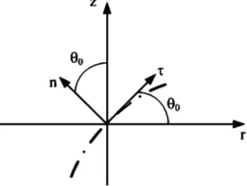
A. Modeling particle velocity using Gaussian beams Let consider the general geometry of the tangent共␶兲 and the normal共n兲 ray unitary vectors, at a particular point of a ray trajectory, as shown by the dashdot line in Fig.1.

Particle velocity 共v兲 can be calculated from the linear acoustic equation共Euler’s equation兲 through the relationship with the acoustic pressure as:

v = − i

␻␳ⵜ p, 共1兲

where␳ represents the density of the watercolumn and␻is the working frequency of the propagating acoustic wave. The pressure gradientⵜp at a particular point of the ray trajectory can be expressed as:

ⵜp =

冋

⳵s,

⳵p

⳵N

册

where⳵p/⳵s and⳵p/⳵N stand for the derivative along␶ and

n, respectively, N is the normal distance from the ray, s is the

FIG. 1. Diagram of the ray trajectory共dashdot line兲 with ray unitary vectors

␶and n projections onto the horizontal r and vertical z axes.

arclength along the ray and the ray unitary vectors at that point are given by:

␶=关cos␪0,sin␪0兴 and n = 关− sin␪0,cos␪0兴, 共3兲

where ␪0 is the angle between the 共r,z兲 axes and the ray

unitary vectors.

Hence, the horizontal and vertical particle velocity com-ponents共vr,vz兲 are obtained by projecting the pressure

gra-dient onto the共r,z兲 axes as:

vr= ⳵p ⳵scos␪0− ⳵p ⳵Nsin␪0 and vz= ⳵p ⳵ssin␪0 + ⳵p ⳵Ncos␪0. 共4兲

While the VSA has three components thevxandvy

com-ponents are calculated by projecting the horizontal particle velocity in the azimuthal direction of the source共␸S兲,

previ-ously estimated, then:

vx=vrcos共␸S兲 and vy=vrsin共␸S兲. 共5兲

Using the Gaussian beam approximation of the ray pres-sure given by18,19 p共s,N兲 = P0共s兲exp

冋

冉

冊

册

where c共s兲 is the sound speed at position s, P0共s兲 is an

arbi-trary constant and ␥共s兲 is related to beamwidth and curvature.19

The analytical expressions for the pressure gradient components corresponds to:

⳵p ⳵s = − i ␻ cp and ⳵p ⳵N= − i␻␥共s兲Np. 共7兲

Assuming a small aperture array and a generic set of environmental parameters共⌰0兲 that characterize the channel,

including ocean bottom parameters, the particle velocity can be written as: v共⌰0兲 = u共⌰0兲p, 共8兲 where u共⌰₀兲 =

冤

冥

冤

冥

is the vector defined for a ray trajectory 共␪₀兲. In a real sce-nario, not only one ray but several rays impinge the array. In this case u共⌰₀兲 in Eq.共8兲 is defined as a sum of the contri-butions of each ray.

B. Data model

Assuming that the propagation channel is a linear time-invariant system, p is the acoustic pressure andvx,vyandvz

are the three particle velocity components, then the field measured at the vector sensor due to a source signal s共t兲 is given by:

yk共t,⌰0兲 = hk共t,⌰0兲 ⴱ s共t兲 + nk共t兲, 共10兲

where ⴱ denotes convolution, ⌰0 is a parameter vector, hk共⌰0兲 is the channel impulse response and nk共t兲 is the

addi-tive noise for pressure and the three components of particle velocity for k = p ,vx,vy,vz, respectively.

Assuming a narrowband signal, the sensor output at a frequency␻ 共omitting the frequency dependency in the fol-lowing兲 for a particular set of channel parameters ⌰0can be

rewritten as:

yk共⌰0兲 = hk共⌰0兲s + nk, 共11兲

where s is the source component at frequency ␻, hk共⌰0兲 is

the channel response and nkis the additive noise.

Taking into account Eq. 共8兲 and 共9兲, the vector sensor model can be obtained as:

冤

冥

冤

冥

冤

冥

In the following it is assumed that the additive noise is zero mean, white, both in time and space,20with variance␴n2

and uncorrelated with the signal s, itself with zero mean and variance␴s

2

.

For an array of L vector sensors, the acoustic pressure at frequency␻is given by:

yp共⌰0兲 = 关yp₁共⌰0兲, ¯ ,yp_L共⌰0兲兴T, 共13兲

where yp_l共⌰0兲 is the acoustic pressure at the lth vector

sen-sor. The linear data model for the acoustic pressure is: yp共⌰0兲 = hp共⌰0兲s + np, 共14兲

where hp共⌰0兲 is the channel frequency response at L

pres-sure sensors and npis the additive acoustic pressure noise.

A similar definition has been adopted for the particle velocity, where the velocity part of the measurement is

yv共⌰0兲 = 关yv_x1共⌰0兲, ¯ ,yv_xL共⌰0兲,yv_y1共⌰0兲, ¯ ,

yv_yL共⌰0兲,yv_z1共⌰0兲, ¯ ,yv_zL共⌰0兲兴T. 共15兲

Considering short arrays, u共⌰0兲 is assumed to be

ap-proximately constant for all elements thus, the data model for the particle velocity components is given by:

yv共⌰0兲 = u共⌰0兲丢hp共⌰0兲s + nv, 共16兲

where n_vis the additive noise satisfying the above assump-tions and 丢 is the Kronecker product. For hp共⌰0兲 with

Combining Eq. 共14兲 and 共16兲 a complete VSA data model, formed by the acoustic pressure and the particle ve-locity, can be defined for a signal measured on L vector sensor elements as:

y_pv共⌰₀兲 =

冋

册

冋

册

冋

册

resulting in a 4L⫻1 dimensional data model.

C. Bartlett estimator

The classical Bartlett estimator is possibly the most widely used technique for parameter estimation in signal processing, usually expressed in terms of the acoustic pressure.21

The Bartlett parameter estimate⌰ˆ0is given as the

argu-ment of the maximum of the function:

PB,p共⌰兲 = E兵eˆp H_共⌰兲y

p共⌰0兲yp H_共⌰

0兲eˆp共⌰兲其, 共18兲

where yp共⌰0兲 is the measured acoustic pressure data and the

replica vector estimator eˆp共⌰0兲 defined as the vector ep共⌰兲

that maximizes the mean quadratic power: eˆp共⌰兲 = arg max

e_p共⌰兲,⌰⑀⍀ ep H_共⌰兲R p共⌰0兲ep共⌰兲, 共19兲 subject to ep H_共⌰兲e

p共⌰兲=1, where 共.兲Hrepresents the complex

conjugated transposed operator, ⍀ is the parameter space,

E兵.其 denotes statistical expectation and Rp共⌰0兲

= E兵yp共⌰0兲yp H_共⌰

0兲其 is the correlation matrix.

In practice the correlation matrix Rp共⌰0兲 is usually

un-known, thus a correlation matrix estimator Rˆp共⌰0兲 is

ob-tained by: Rˆp共⌰0兲 = 1 K

兺

assuming that there are K data snapshots available.

Considering the acoustic pressure data model Eq. 共14兲, the correlation matrix Rp共⌰0兲 can be written as:

Rp共⌰0兲 = hp共⌰0兲hp H_共⌰ 0兲␴s 2 +␴n 2 I. 共21兲

Therefore, a possible estimator eˆp共⌰兲 of ep共⌰兲 is

ob-tained as:

eˆp共⌰兲 = arg max

e_p共⌰兲,⌰⑀⍀兵ep H_共⌰兲R p共⌰0兲ep共⌰兲其, 共22兲 subject to ep H_共⌰兲e p共⌰兲=1. According to 共21兲 it can be

shown that the well-known nontrivial solution22,23is

eˆp共⌰兲 = hp共⌰兲

冑

where the denominator is a scalar normalization and hp共⌰兲

contains the replica of the signal structure as “seen” by the receiver.

Replacing 共23兲 and 共21兲 in the generic estimator 共18兲 provides the Bartlett estimator for acoustic pressure共p-only兲 of any search parameter⌰:

PB,p共⌰兲 = hp H_共⌰兲R p共⌰0兲hp共⌰兲 hp H_共⌰兲h p共⌰兲 =hp H_共⌰兲h p共⌰0兲hp H_共⌰ 0兲hp共⌰兲 hp H_共⌰兲h p共⌰兲 ␴s2+␴n2 = Bp共⌰兲␴s2+␴n2, 共24兲

where Bp共⌰兲 is the noise-free pressure beampattern 共0

ⱕBp共⌰兲ⱕ1兲, with the parameter estimator given by:

⌰ˆ = arg max

⌰⑀⍀ PB,p共⌰兲. 共25兲

The derivation of the Bartlett estimator for particle ve-locity only共v-only兲 and for full VSA 共p+v兲 can be done by taking into account the data model共16兲,共17兲and the maxi-mization of the replica vector presented in the Appendix. Thus, the Bartlett estimator forv-only outputs can be written

as: P_B,v共⌰兲 =关u H_{共⌰兲u共⌰} 0兲兴2 uH共⌰兲u共⌰兲 Bp共⌰兲␴s 2_+␴ n 2 ⬀ 关cos2_{共␦兲兴P} B,p共⌰兲, 共26兲

where Bp共⌰兲 is the beampattern for p-only defined in共24兲,␦

is the angle between the replica vector u共⌰兲 and the data vector u共⌰₀兲, considering that the inner product between two vectors is proportional to the cosine of the angle between these vectors. Based on 共26兲, one can conclude that the

v-only Bartlett estimator response is proportional to the p-only Bartlett response, where the inner product uH_{共⌰兲u共⌰}

0兲 is the constant of proportionality herein called

directivity factor. This directivity factor provides an im-proved sidelobe reduction or sidelobe suppression when compared with the p-only Bartlett response and contributes to improving the resolution of the parameter estimation.

The effect of merging the acoustic pressure and the par-ticle velocity components in the previously derived Bartlett estimator gives the VSA共p+v兲 Bartlett estimator, defined as

PB,pv共⌰兲 =

冉

冋

册

冋

册

冊

冋

册

冋

册

冋

冉

冊

册

One can conclude that when the VSA共p+v兲 estimator is considered, the estimate function is proportional to 关4 cos4_{共␦/2兲兴 providing a wider main lobe, shown in共27兲, as}

compared to the estimator with v-only共26兲. This is due to the cosine of the half angle. Moreover, the inclusion of the pressure on the estimator eliminates the ambiguities caused by the关cos2_{共␦兲兴 even when frequencies higher than the array}

design frequency are used. This behavior is illustrated with simulations in the next section.

III. SIMULATION RESULTS

In order to illustrate the advantage of vector sensors in parameter estimation using the VSA Bartlett estimator, two applications are discussed: direction of arrival 共DOA兲 esti-mation and matched-field inversion 共MFI兲 for ocean bottom properties estimation. The TRACE Gaussian beam model18 is used to generate the replica field. This model was designed to perform two dimensional acoustic ray tracing in ocean waveguides and provides different sets of output information such as the acoustic pressure and the particle velocity com-ponents.

A. DOA estimation

The main advantage of the VSA in DOA estimation is that it resolves both vertical and azimuthal directions with a linear array. The plane wave beamformer is applied to com-pare the performance of the VSA with that of pressure sensor arrays, where the individual sensor outputs are delayed, weighted and summed in a conventional manner. In the case of plane wave DOA estimation, the search parameter⌰ is the direction 共␪S,␾S兲, where ␪S is the azimuth angle and ␾S is

the elevation angle. The replica vectors in 共24兲, 共26兲, and

共27兲are simple combinations of weights, which are direction cosines for the particle velocity components and unity for pressure. These are, respectively given by:

• considering pressure only:

ep共␪S,␾S兲 = exp共ikជS. rជ兲, 共28兲

• considering particle velocity components only:

ev共␪S,␾S兲 = 关u共␪S,␾S兲兴T丢exp共ikជS. rជ兲, 共29兲

where the weigthing vector is u共␪S,␾S兲

=关cos共␪S兲sin共␾S兲 sin共␪S兲sin共␾S兲 cos共␾S兲兴T,

• and for both pressure and particle velocity:

epv共␪S,␾S兲 =

关

兴

where kជSis the wavenumber vector corresponding to the

cho-sen steering angle, or look direction 共␪S,␾S兲 of the array,

␪S苸关−␲;␲兴,␾S苸关−␲/2;␲/2兴 and rជ is the position vector

of the VSA elements as shown in Fig.2.

The VSA has four equally spaced elements共with 10 cm spacing兲 and is located along the z-axis, with the first ele-ment at the origin of the cartesian coordinates system 共Fig.

2兲. The simulation results were obtained for the array design

frequency, 7500 Hz, and for a true source DOA of␪S= 45 °

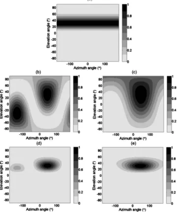
and␾S= 30 °. Figure 3presents the simulation results when

Eqs.共24兲,共26兲, and共27兲are applied to DOA estimation. Figure 3共a兲illustrates the results when the p-only esti-mator is considered, using 共24兲. Since the array is placed along the vertical axis, only the elevation angle is resolved due to the omnidirectionality of the pressure sensors. Figure

3共b兲 and 3共c兲 present the results for the directivity factors 关cos2_{共␦兲兴 and 关4 cos}4_{共␦/2兲兴 in 共26兲 and 共27兲, respectively,}

where␦is the angle between the replica and the data vector 共Section II C兲. It can be seen that the ambiguity presented in Fig.3共b兲is eliminated when关4 cos4共␦/2兲兴 is used 关Fig.3共c兲兴, due to the cosine of the half angle. Figure 3共d兲 shows the results of the Bartlett estimator usingv-only—this yields the

best resolution in both azimuth and elevation, but produces a low amplitude ambiguity at an azimuth of共⫺135°兲. On the other hand, the VSA 共p+v兲 Bartlett estimator has a wider main lobe without ambiguities, as shown in Fig.3共e兲, and the DOA is resolved in both elevation and azimuth. The results presented in Fig.3共d兲and3共e兲are obtained by Eqs.共26兲and

共27兲, but they can be seen by visual superposition of Fig.3共a兲 with Figs. 3共b兲 and 3共c兲, respectively. Both directions are resolved and the conjugation of the acoustic pressure with the particle velocity eliminates the ambiguity with an array of only a few elements.

FIG. 2. Array coordinates and geometry of acoustic plane wave propaga-tion, with azimuth共␪S兲 and elevation 共␾S兲 angles. The vector sensor ele-ments are located in the z-axis with the first element at the origin of the cartesian coordinate system.

FIG. 3. DOA estimation simulation results at frequency 7500 Hz with azi-muth共␪S= 45°兲 and elevation 共␾S= 30°兲 angles using the normalized Bartlett beamformer considering:共a兲 p-only response, 共b兲 the 关cos2_共␦_{兲兴 of Eq.共26兲,} 共c兲 the 关4 cos4_{共␦/2兲兴 of Eq.共27兲,共d兲 v-only 共26兲, and 共e兲 all sensors VSA} 共p+v兲共27兲.

B. Ocean bottom properties MFI

The simulation scenario is shown in Fig. 4 and is par-tially based on the Makai experimental setup共for which re-sults on experiment data will be presented in Section IV兲. This environment has a deep mixed layer, characteristic of Hawaii, and the bathymetry at the site is range independent with a water depth of 104 m. The source is bottom moored at 98 m depth and 1830 m range. The results are obtained with a four element共10 cm spacing兲 VSA deployed with the deep-est element positioned at 79.9 m. The frequency of 13078 Hz is considered in the simulations.

A common approach in acoustic inversion is to consider

both geometrical and environmental parameters as candi-dates for inversion. However, during the Makai experiment the system geometry was known to a degree of accuracy that allowed to consider only environmental inversion while keeping fixed the geometrical parameters. Moreover, since the objective is seabed characterization and the Makai data set can be well described with a simplified three parameter seabed model, the seabed parameters to be considered herein are sediment compressional speed共cp兲, density 共␳兲 and

com-pressional attenuation 共␣p兲. These parameters are estimated

taking into account the particle velocity outputs and a MFI processor based on the Bartlett estimators presented in Sec-tion II C. The field replicas are generated using the TRACE Gaussian beam model18for a half space seabed.

Preliminary tests have shown that the MFI processor is decreasingly sensitive to sediment compressional speed, den-sity and nearly insensitive to compressional attenuation. Therefore the parameter space was reduced to the most sen-sitive parameters: sediment compressional speed and density. The true values for the seabed parameters considered in the simulation were taken as: cp= 1575 m/s,␳= 1.5 g/cm3 and

␣p= 0.6 dB/␭. To illustrate and to compare the resolution of

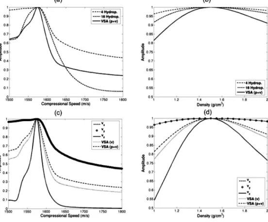
the several seabed parameter estimators previously defined, Fig.5presents the ambiguity surfaces 1D cross sections for each parameter.

Figure 5共a兲 and 5共b兲 compare the estimation perfor-mance obtained considering the p-only关Eq. 共24兲兴 for 4 and 16 pressure sensors and the VSA共p+v兲 关Eq.共27兲兴, for sedi-FIG. 4. Simulation scenario based on the typical setup encountered during

the Makai experiment with a very large mixed layer, characteristic of Ha-waii. The source is bottom moored at 98 m depth and 1830 m range. The VSA is deployed with the deepest element at 79.9 m.

FIG. 5. Seabed parameters estimation simulation results obtained with the normalized Bartlett estimator at frequency 13078 Hz and for␣= 0.6 dB/␭ for 关共a兲 and共c兲兴 sediment compressional speed where␳= 1.5 g/cm3_{and关共b兲 and 共d兲兴 density where c}

p= 1575 m/s. The simulation results were obtained comparing: the p-only Bartlett estimator response共24兲 for 4 and 16 pressure sensors with VSA 共p+v兲 Bartlett estimator response 共27兲 共a兲 and 共b兲 and the Bartlett estimator response considering: individual data components共vx,vyandvz兲, v-only Bartlett estimator 共VSA 共v兲兲 and all sensors 共VSA 共p+v兲兲 共c兲 and 共d兲.

ment compressional speed and density, respectively. The scope of comparing the 4-element VSA with a 4 and 16 pressure sensor array is to consider an equal aperture com-parison in the former and an equal number of sensors in the later. The figures show that the VSA improves the resolution in both sediment compressional speed and density, when compared with 4 and 16 pressure sensors. The results suggest that the VSA can offer a significant array size reduction with a better performance when compared with a pressure sensor array.

Figure 5共c兲 and 5共d兲 show the estimation results, ob-tained respectively, for sediment compressional speed and density, considering the Bartlett estimator for: individual par-ticle velocity component,v-only and VSA共p+v兲. The plots

obtained for horizontal particle velocity components vx

共dashed line兲 and vy共circles兲 are coincident, since these

com-ponents mostly depend on low-order modes, thus having little or no interaction with the bottom. On the other hand, the vertical componentvz共solid line兲 has a higher sensitivity

to bottom structure than thevxandvycomponents, since it is

influenced by the high-order modes with a larger contribu-tion to the vertical particle velocity due to their grazing angle.11The results suggest that both seabed parameters can be obtained using only the vertical component of the particle velocity. Comparing the VSA Bartlett outputs VSA共v兲 and VSA共p+v兲, the former 关dotted curve in Fig.5共c兲and5共d兲兴 has a narrower main lobe than the later共dashdot curve兲 due to the cosine function of the half angle,关Eq.共27兲兴, similarly to the result obtained in DOA estimation. One can conclude that a VSA increases significantly the resolution of the sea-bed parameters: sediment compressional speed and density.

IV. EXPERIMENTAL RESULTS A. Experimental setup

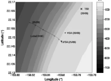
The data analyzed here were acquired during the Makai Experiment that took place from September 15th to October 2nd 2005, on the North West coast of Kauai I., Hawaii, USA.15Figure6shows the bathymetry map of the MakaiEx

area, showing a smooth and uniform area of depth around 80–100 m accompanying the island bathymetric contour, sur-rounded by the continental relatively steep slope to the deeper ocean to the West. Extensive ground truth measure-ments were carried out in this area during previous experi-ments and showed that most of the bottom in the area is covered with coral sands over a basalt hard bottom. The sound velocity in coral sands should be approximately 1700 m/s and the sediment thickness is unknown but expected to be on the order of a fraction of a meter in most places.

The four-element 10 cm spacing vertical VSA was de-ployed twice, on September 20th and 25th and acquired data from two different acoustic sources: the TB2 testbed and the Lubell916C, respectively. Figure6also shows the equipment location: on September 20th, the VSA and TB2 were in a fixed-fixed configuration over a range independent bathym-etry with water depth of approximately 104 m; on September 25th, the VSA was fixed and the Lubell 916C was towed toward the VSA by a small inflatable boat at a depth of 10 m starting at a range of 2300 m共track marked Lubell916C兲.

On September 20th, the experimental baseline environ-ment with the mean sound speed profile considered for this day is identical to that shown in Fig. 4. The VSA was de-ployed with the deepest element at 79.9 m depth and the source TB2 was bottom moored at 98 m depth and 1830 m range. The experimental setup used in September 25th, is shown in Fig.7, where the VSA was deployed with the deep-est element at 40 m depth. The Lubell 916C source ap-proached the VSA from 2300 m range but the data consid-ered herein was taken at 300 m range, where the water depth varies from 119 m at the source location to 104 m at the VSA. On September 20th, the TB2 source transmitted linear frequency modulation sweeps 共LFMs兲, tone combs and M-sequences in the 8–14 kHz band, while only the tone combs were used in the processing for this day. On Septem-ber 25th, the Lubell 916C source transmitted sequences of controlled waveforms—of these, the 50 ms LFM pulses spanning the 8–14 kHz band were processed.

B. Seabed parameter estimation

The estimation of seabed parameters is performed using two different methods. First, taking advantage of the spatial FIG. 6. Bathymetry map of the Makai Experiment area with the location of

the VSA for the two deployments共September 20th and 25th兲 as well as the location of the acoustic sources TB2共fixed兲 and Lubell916C 共track兲.

FIG. 7. Baseline environment on September 25th 2005 with mean sound speed profile. The VSA was deployed with the deepest element at 40 m and the Lubell916C source was towed from a boat at 10 m depth.

filtering capabilities and directionality of the VSA, the sea-bed parameters and layer structure is estimated comparing the reflection loss of experimental data to the reflection loss modeled by SAFARI model.24 Second, the seabed param-eters are estimated using MFI comparing several Bartlett es-timators previously derived.

1. Bottom reflection loss

C. Harrison25proposed an estimation technique for bot-tom reflection loss, using vertical pressure sensor array mea-surements of surface generated noise. The estimation of bot-tom reflection loss versus grazing angle for the signal bandwidth is obtained by dividing the down and upward en-ergy reaching the array. This technique can be adapted for vertical measurements of an azimuthal direction of acoustic sources with a small aperture VSA, taking advantage of its spatial filtering capabilities. The bottom reflection loss de-duced from experimental data is then compared to the reflec-tion loss modeled by the SAFARI model, for a given set of parameters for sediment and/or bottom: compressional wave speed cp, shear wave speed cS, compressional wave

attenua-tion ␣p, shear attenuation␣Sand density ␳. The best

agree-ment gives an estimate of bottom layering structure together with its most characteristic physical parameters.

Let us consider an emitted signal S in a range indepen-dent environment, where the localization is a function of elevation angle ␾ and azimuth ␪. The array beam pattern

B共␪,␾兲 for the source look direction was estimated taking into account the plane wave beamforming described in Sec-tion III A. Then, the array beam pattern for an azimuthal direction ␪, shown in Fig.8, is given by the vertical beam response A共␾0兲 for each steer angle ␾0. According to25 the

ratio between the downward and upward beam responses is an approximation of the bottom reflection coefficient Rb:

A共−␾0兲 A共+␾0兲

= Rb共␾b共␾0兲兲, 共31兲

where the angle measured by beamforming at the receiver

␾0, is corrected to the angle at the seabed␾b, in agreement to

the sound-speed profile by Snell’s law.

␾b= arccos

冋

冉

冊

cos共␾0兲

册

where cband crare the sound speed at the bottom and at the

receiver, respectively.

Figure 9 presents the vertical beam response for each frequency extracted for the source azimuthal direction of in-terest, considering both p-only Fig.9共a兲and VSA共p+v兲 Fig.

9共b兲. As it can be seen in Fig.9共a兲, the beam response in the

p-only case is nearly symmetric for both negative and

posi-tive elevation angles 共up and down, respectively兲, resulting in a poor information about the bottom attenuation. Compar-ing with the directional case, Fig. 9共b兲, the vertical beam response clearly differentiates up and downward energy. This allows for retrieving bottom information, since the vertical component of the VSA is constituted by the rays with strong interactions with the seabed. This is clearly a unique capa-bility resulting from the processing gain provided by vector sensors.

Dividing the down to up beam responses for the same elevation angle, the frequency versus bottom angle reflection losses curves were obtained for the signals acquired on Sep-tember 25th and then compared with the reflection loss curves modeled by the SAFARI model,24 using a trial and error approach. Initial values of the parameters were found in the literature based on available qualitative description of the area.19 Then, manual adjustments were made to estimate a reflection loss figure similar to that obtained with measured data. It was observed that the most relevant parameters are FIG. 8. Sketch of the ray approached geometry of a plane wave emitted by

source共S兲 and received by the receiver 共R兲 at the elevation angle␾0.

FIG. 9. Beam response at source azimuthal direction obtained using共a兲 the 4 p-only sensors of the VSA and共b兲 all sensors VSA 共p+v兲.

the layer thickness, an important parameter for fringe sepa-ration agreement, and the sound speed on the various layers and in the half-space, which influences the critical angles of the form:

␾c_i= arccos

冉

冊

, 共33兲

where cWis the water sound speed near the water sediment

interface and cs_i is the ith sediment or sub-bottom sound

speed.

Figure 10共a兲 and 10共b兲 presents the bottom reflection loss deduced from the down-up ratio of the experimental data and that modeled by the SAFARI model, respectively. This structure suggests that the area can be modeled as a four-layer environment 共three boundaries兲: water, two sedi-ments and the bottom half space. Three critical angles are presented in Fig. 10共a兲: ␾c₁⯝13 °, ␾c₂⯝26 ° and ␾c₃

⯝49 ° and according to共33兲where the water sound speed is

cW= 1530 m/s, the sediment and sub-bottom sound speeds

can be calculated: cs₁= 1570 m/s, cs₂= 1700 m/s and cs₃

= 2330 m/s. Figure 10共b兲 presents the reflection loss mod-eled with the same features as those observed in the experi-mental data, Fig. 10共a兲. Table I presents the results of the estimated bottom structure taking into account the real data and manual adjustments on the SAFARI model. The same fringe separation appears for a layer thickness of 0.175 m and this is in line with the ground truth 共see Section IV A兲 but the first sediment sound speed is different from 1700 m/s, however, the sediment sound speed of cs= 1570 m/s is in

line with the results obtained by MFI in the next section. One can conclude that the three-layer environment suggested in15 could be in fact a four-layer environment 共water, soft sedi-ment, sand and basalt兲 with a soft sediment over the sand. Due to the small value of the thickness of this first sediment, it was not considered in the descriptive ground truth mea-surements共see Section IV A兲.

2. MFI results

The vector sensor based MFI method discussed in Sec-tions II C and III is applied to the data measured by the VSA on September 20th. In the simulation section it was found that compressional attenuation is the parameter with the least sensitivity and therefore the most difficult to invert for. Ex-tensive runs were made for determining the most likely value for compressional attenuation within the range of 0.1 to 0.9 dB/␭ and a best match was found for the value of 0.6 dB/␭, which was then used as a fixed parameter in the sequel.

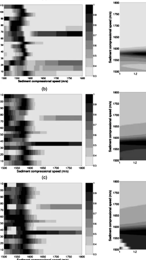
Figure 11 shows the ambiguity surfaces cross sections for sediment compressional speed obtained for the maximum density values of the estimator functions throughout almost two hours. Figure 11共a兲–11共c兲were obtained with the Bar-tlett estimators:关Eq.共26兲兴 with the vertical component only,

v-only 关Eq. 共26兲兴 and VSA 共p+v兲 关Eq. 共27兲兴, respectively.

These plots show the stability of the results during the data acquisition period 共approximately 2 h兲 and give an estima-tion of sediment compressional speed of approximately 1575 m/s. As already seen in the simulations, the vertical compo-nent has also a narrow main lobe due to the higher sensitivity to bottom structure, Fig. 11共a兲. On the other hand, the VSA 共p+v兲 estimator, Fig.11共c兲, has a wider main lobe than the

v-only estimator, Fig. 11共b兲, confirming the simulations and the analytical results obtained. The results are generically in good agreement with those obtained in the previous section. FIG. 10. Bottom reflection loss: deduced from the down-up ratio of the

experimental data共a兲 and modeled by the SAFARI model 共b兲.

TABLE I. Estimatted bottom parameters taking into account the measured VSA data on September 25th and manual adjustments on SAFARI model, considering four layer structure.

Sediment First layer Second layer Sub-bottom

Thickness共m兲 0.175 20 ¯ ␳共g/cm3_{兲 1.6 2.1 2.1} cp共m/s兲 1570 1700 2330 cS共m/s兲 67 700 1000 ␣p共dB/␭兲 0.6 0.1 0.1 ␣S共dB/␭兲 1.0 0.2 0.2

Figure12 shows the ambiguity surface for both seabed parameters and was obtained for the same estimator cases as in Fig.11, using the geometric mean of the estimates along

the data acquisition period. Figure12共a兲shows the ambiguity surface considering关Eq.共26兲兴 with only the vertical compo-nent of the particle velocity which points to values for den-FIG. 12. Measured data normalized ambiguity surfaces for sediment com-pressional speed and density, using the geometric mean of estimates along the acquisition period, for:共a兲 Bartlett vertical component only, 共b兲 Bartlett VSA共v兲 and 共c兲 Bartlett VSA 共p+v兲.

FIG. 11. Measured data normalized ambiguity surfaces for sediment com-pressional speed during data acquisition period, for:共a兲 Bartlett vertical component,共b兲 Bartlett VSA 共v兲 and 共c兲 Bartlett VSA 共p+v兲.

sity of approximately 1.4 g/cm3 and this component has a narrower main lobe. The VSA Bartlett estimators,关Eq.共26兲兴 and关Eq.共27兲兴, respectively Fig.12共b兲and12共c兲confirm this result but with wider main lobes. The results show that the density can be estimated with higher resolution using a small VSA than using a small pressure sensor array, and agree with the results obtained for bottom reflection loss 共Section IV B 1兲.

V. CONCLUSIONS

In recent years, acoustic particle velocity sensors have been introduced and discussed by several authors, mainly in the DOA estimation context. In this paper, the possibility of using a vertical VSA and active signals in the 8–14 kHz band to estimate bottom properties, beyond DOA estimation was presented. The original contributions of this work consist in the following: a vector sensor measurement model was de-veloped, which allowed to introduce the particle velocity in the Bartlett estimator; it was demonstrated with two different estimation techniques, that the inclusion of the particle ve-locity information improves the resolution of the seabed pa-rameter estimation; finally that good results can be obtained using only the vertical particle velocity component.

The determination of the bottom reflection coefficient deduced by the ratio of the downward and upward beam response25 using 8–14 kHz band measured data became a simple method for estimating the bottom structure and re-spective geoacoustic parameters. The unique capability of the VSA for vertical beam response information extraction, when compared with the performance of a pressure sensor array with the same aperture, was demonstrated. The reflec-tion loss curves observed with the measured data were com-pared with the reflection loss curves predicted by the SA-FARI model, which allowed to define the number of layers, their thickness and their geoacoustic parameters.

The proposed inversion based on VSA matched-field processing were used to estimate the values of the sediment parameters: sediment compressional speed, density and com-pressional attenuation. The classical Bartlett estimator adapted to vector sensor information provides better results for seabed parameter estimation than pressure sensor arrays of the same length. The estimates of sediment compressional speed produced from the vertical particle velocity component had high resolution and were consistent over a significant time interval. Furthermore, the VSA-based measurements also produced reliable estimates of sediment density and compressional attenuation. Note that these parameters are normally difficult to estimate with pressure measurements alone. An interesting and perhaps surprising outcome of this work was that the channel impulse response has sufficient structure to support estimation of seabed geoacoustic param-eters in this high-frequency band. The results are compatible with those obtained with the bottom reflection curves and with the historical data of the area.

The particle velocity information enhances DOA and seabed geoacoustic parameter estimation, resulting in a bet-ter paramebet-ter resolution. The usage of VSA at

high-frequency provides an alternative for a compact and easy-to-deploy system in various underwater acoustical applications.

ACKNOWLEDGMENTS

The authors would like to thank Michael Porter, chief scientist for the Makai Experiment and Jerry Tarasek at Na-val Surface Weapons Center for the loan of the vector sensor array used in the experiment. The authors also thank Bruce Abraham at Applied Physical Sciences for providing assis-tance with the data acquisition and the team at HLS Re-search, particularly Paul Hursky for their help with the data processed in this work. This work was partially supported by the project SENSOCEAN funded by FCT programme PTDC/EEA-ELC/104561/2008.

APPENDIX: DERIVATION OF THE BARTLETT ESTIMATOR FOR PARTICLE VELOCITY

For the derivation of the Bartlett estimator taking into account the particle velocity components, the following properties of the Kronecker product are considered:

1. A丢共aB兲=共aA兲丢B = a共A丢B兲 where a is a scalar, 2. 共A丢B兲H_{= A}H_丢BH_,

3. 共A丢B兲共C丢D兲=AC丢BD

4. if A₁, A₂,¯ ,Ap are M⫻M and B1, B2,¯ ,Bp are N

⫻N then 共A1丢B1兲共A2丢B2兲¯共Ap丢Bp兲=共A1A2¯Ap兲 丢共B1B2¯Bp兲.

In the following, v共⌰0,⌰兲=u共⌰0,⌰兲 when only particle

velocity components are considered in the data model—v-only; or v共⌰0,⌰兲=关1 u共⌰0,⌰兲兴T when both

pressure and particle velocity components are considered— VSA 共p+v兲. For simplicity, the following notation v共⌰0兲 →v0and v共⌰兲→v are used.

The correlation matrix R0depending on the particle

ve-locity data model, with or without pressure, can be written as: R0=关v0丢h0p兴关v0丢h0p兴H␴s 2 +␴n 2 I, 共A1兲

where the additive noise is zero mean, white both in time and space, with variance ␴_n2 and uncorrelated with the signal s, itself with zero mean and variance ␴_s2, h0p is the channel

frequency response at the L pressure sensors and v0 is the

data vector.

A possible estimator eˆ of e is obtained as:

eˆ = arg max

e 兵e

H

R0e其, 共A2兲

subject to eHe = 1.

Using the eigen decomposition of the correlation matrix associated with the signal and noise subspaces according to structure共A1兲and for this case in particular, it can be shown that v0丢h0p is one of the eigenvectors of R0, since

post-multiplying共A1兲by this eigenvector and using the properties of the Kronecker product 2 and 3, gives:

R0关v0丢h0p兴 = 兵关v0丢h0p兴关v0 H 丢h0p H_兴␴ s 2_+␴ n 2_I其关v 0丢h0p兴 =关v0丢h0p兴关v0 H v0丢h0p H h0p兴␴s 2 +␴n 2_关v 0 丢h0p兴 = 关v0丢h0p兴兵v0 2 h0p 2 _␴ s 2 +␴n 2_{其, 共A3兲}

where the quantity in brackets 兵其 is simply the eigenvalue associated with this eigenvector. Then a maximization with respect to e is the eigenvector associated with the largest eigenvalue as given by:

eˆ =

_冑

_冑

_冑

where eˆp is the replica vector estimator for the pressure

de-fined in Section II C and where properties 2 and 3 were used. Replacing共A4兲and共A1兲 in the generic Bartlett estima-tor共18兲, using the properties of the Kronecker product 2, 3 and 4 with subject to e_pHep= 1, the Bartlett estimator for the

particle velocity model is given by:

PB= vH

冑

冑

Taking into account共24兲, one can conclude that the vec-tor sensor estimavec-tor 共with or without pressure兲 is propor-tional to the acoustic pressure estimator response, where the inner product vH_v

0 is the constant of proportionality herein

called directivity factor.

1_{A. Nehorai and E. Paldi, “Acoustic vector-sensor array processing,” IEEE} Trans. Signal Process. 42, 2481–2491共1994兲.

2_{B. A. Cray and A. H. Nuttall, “Directivity factors for linear arrays of} velocity sensors,” J. Acoust. Soc. Am. 110, 324–331共2001兲.

3_{J. Tabrikian, R. Shavit, and D. Rahamim, “An efficient vector sensor} con-figuration for source localization,” IEEE Signal Process. Lett. 11, 690–693 共2004兲.

4_{C. Wan, A. Kong, and C. Liu, “A comparative study of doa estimation} using vector/gradient sensors,” in Proceedings of Oceans 2006, Asia Pa-cific共2007兲, pp. 1–4.

5_{J. C. Shipps and B. M. Abraham, “The use of vector sensors for} under-water port and under-waterway security,” in Proceedings of the Sensors for Industry Conference, New Orleans, LA共2004兲, pp. 41–44.

6_{D. Lindwall, “Marine seismic surveys with vector acoustic sensors,” in} Proceedings of the Society of Exploration Geophysicists Annual Meeting,

New Orleans, LA共2006兲, pp. 1208–1212.

7_{Y. H. Wang, J. Q. Zhang, B. Hu, and J. He, “Hypercomplex model of} acoustic vector sensor array with its application for the high resolution two dimensional direction of arrival estimation,” in Proceedings of the I2_MTC 2008, IEEE International Instrumentation and Measurement Technology Conference, Victoria, Vancouver, Canada共2008兲, pp. 1–5.

8_{S. Miron, N. Le Bihan, and J. I. Mars, “Quaternion-music for} vector-sensor array processing,” IEEE Trans. Signal Process. 54, 1218–1229 共2006兲.

9_{A. Abdi, H. Guo, and P. Sutthiwan, “A new vector sensor receiver for} underwater acoustic communication,” in Proceedings of MTS/IEEE Oceans, Vancouver, BC, Canada共2007兲, pp. 1–10.

10_{A. Song, M. Badiey, P. Hursky, and A. Abdi, “Time reversal receivers for} underwater acoustic communication using vector sensors,” in Proceedings of MTS/IEEE Oceans, Quebec, Canada共2008兲, pp. 1–10.

11_{H. Peng and F. Li, “Geoacoustic inversion based on a vector hydrophone} array,” Chin. Phys. Lett. 24, 1997–1980共2007兲.

12_{M. J. Hinich, “Maximum-likelihood signal processing for a vertical} ar-ray,” J. Acoust. Soc. Am. 54, 499–503共1973兲.

13_{P. Gerstoft, “Inversion of seismoacoustic data using genetic algorithms} and a posteriori probability distributions,” J. Acoust. Soc. Am. 95, 770– 782共1994兲.

14_{C. E. Lindsay and N. R. Chapman, “Matched-field inversion for} geoacous-tic model parameters using adaptive simulated annealing,” IEEE J. Ocean. Eng. 18, 224–231共1993兲.

15_{M. Porter, B. Abraham, M. Badiey, M. Buckingham, T. Folegot, P.} Hur-sky, S. Jesus, K. Kim, B. Kraft, V. McDonald, C. deMoustier, J. Presig, S. Roy, M. Siderius, H. Song, and W. Yang, “The Makai experiment: High-frequency acoustics,” in Proceedings of the Eighth ECUA, Carvoeiro, Por-tugal共2006兲, edited by S. M. Jesus and O. C. Rodríguez, Vol. 1, pp. 9–18. 16_{P. Santos, P. Felisberto, and P. Hursky, “Source localization with vector} sensor array during the Makai experiment,” in Proceedings of the Second International Conference and Exhibition on Underwater Acoustic Mea-surements: Technologies and Results, pp. 985–990, Heraklion, Greece 共2007兲.

17_{P. Santos, O. C. Rodríguez, P. Felisberto, and S. M. Jesus, “Geoacoustic} matched-field inversion using a vertical vector sensor array,” in Proceed-ings of the Third International Conference and Exhibition on Underwater Acoustic Measurements: Technologies and Results, Nafplion, Greece 共2009兲, pp. 29–34.

18_{O. C. Rodríguez, “The TRACE and TRACEO ray tracing programs,”} http://www.siplab.fct.ualg.pt/models.shtml共Last viewed 6/7/10兲. 19_{F. B. Jensen, W. A. Kuperman, M. B. Porter, and H. Schmidt,}

Computa-tional Ocean Acoustics, AIP Series in Modern Acoustics and Signal Pro-cessing 共American Institute of Physics, Melville, New York, 1994兲, pp. 168–170.

20_{Both between VSA elements and between sensors within each element.} 21_{A. Tolstoy, Matched Field Processing for Underwater Acoustics共World}

Scientific, Singapore, 1993兲, pp. 14–22.

22_{H. Krim and M. Viberg, “Two decades of arraysignal processing} re-search,” IEEE Signal Process. Mag. 13, 67–94共1996兲.

23_{C. Soares and S. M. Jesus, “Broadband matched-field processing:} Coher-ent and incoherCoher-ent approaches,” J. Acoust. Soc. Am. 113, 2587–2598 共2003兲.

24_{H. Schmidt, “SAFARI: Seismo-Acoustic Fast Field Algorithm for} Range-Independent Environments, User’s Guide,” SACLANT Undersea Re-search Centre Report No. SR-113, La Spezia, Italy, 1988.

25_{C. H. Harrison and D. G. Simons, “Geoacoustic inversion of ambient} noise: A simple method,” J. Acoust. Soc. Am. 112, 1377–1387共2002兲.