www.scielo.br/rbg
COMPARATIVE ANALYSES OF GEOPHYSICAL LOGS OF RESISTIVITY
AS APPLIED TO COAL DEPOSITS
Oluwafemi Shekoni Ayodeji, Paulo Salvadoretti, Jo˜ao Felipe Coimbra Leite da Costa,
George Olufunmilayo Gasper and Douglas Marcel Quatiabara Sander Libardi
ABSTRACT.This study compares data sets obtained from three geophysical probes used for measuring rock resistivity. A detailed analysis was carried out to de-termine which of these probes provides the best option in terms of identification of coal-seam thickness. The resistivity probes used were guard log (GL), single-point resistance (SPR), and induction log (IND) probes. To aid the comparison among the different logs, two other geophysical logs were included: natural gamma (NG) and optical televiewer (OPTV), which helped to identify the coal seams. In the specific case of OPTV, when the situation is favorable, it identifies the coal seams and checks the vertical resolution of the other logs. In this study, analyzed data were obtained from four different coal deposits, namely B3, Calombo, Cerro, and Seival. All the coal deposits mentioned are located in the state of Rio Grande do Sul, Brazil. In all, 13 boreholes with recovered core samples are presented and discussed. The geological descriptions of the 13 boreholes are the main information used as a control parameter in comparisons with the geophysical logs, while OPTV images served as an alternative to verify the vertical resolution of the logs. At the end of the analysis, it was found that the guard log probe tends to offer better performance in the aspect of lithological identification, demonstrating a greater capacity in comparison with the others in terms of vertical resolution. Statistically, it presented the closest estimated value of coal-seam thickness in relation to that provided by geological description of the recovered core samples.
Keywords: geophysics, coal, resistivity, OPTV.
RESUMO.Este estudo compara registros de perfilagem geof´ısica obtidos por trˆes sondas que medem a resistividade de litologias. Uma an´alise detalhada foi feita para determinar qual destas sondas proporciona a melhor opc¸˜ao em termos da identificac¸˜ao de espessuras de camadas de carv˜ao. As sondas de resistividade utilizadas foram:guard log,single-point resistanceeinduction log. Para auxiliar na comparac¸˜ao entre as diferentes sondas, outros dois registros geof´ısicos foram inclu´ıdos: radiac¸˜ao gama natural eoptical televiewer(OPTV), os quais ajudaram a identificar os estratos de carv˜ao. No caso espec´ıfico do OPTV, quando a situac¸˜ao ´e favor´avel, ele permite identificar os estratos de carv˜ao e verificar a resoluc¸˜ao vertical dos demais registros. Neste estudo, foram analisados dados obtidos em 4 dep´ositos de carv˜ao diferentes: B3, Calombo, Cerro e Seival. Todos os dep´ositos de carv˜ao mencionados situam-se no estado do Rio Grande do Sul – Brasil. Ao todo, 13 furos de sondagem com recuperac¸˜ao de testemunhos s˜ao apresentados e discutidos. As descric¸˜oes geol´ogicas dos 13 furos de sondagem s˜ao as informac¸˜oes principais utilizadas como parˆametro de controle nas comparac¸˜oes entre os perfis geof´ısicos, enquanto que as imagens OPTV serviram como uma alternativa para verificar a resoluc¸˜ao vertical dos perfis geof´ısicos. Ao final das an´alises, verificou-se que o dispositivoguard logtende a ter o melhor desempenho no aspecto de identificac¸˜ao litol´ogica, demonstrando uma capacidade superior em relac¸˜ao aos demais arranjos em termos de resoluc¸˜ao vertical. Estatisticamente, ele apresentou as estimativas de espessuras mais pr´oximas em valor, em relac¸˜ao `as espessuras proporcionadas pelas descric¸˜oes geol´ogicas de testemunhos de sondagem.
Palavras-chave: geof´ısica, carv˜ao, resistividade, OPTV.
Universidade Federal do Rio Grande do Sul (UFRGS), Laborat´orio de Pesquisa Mineral e Planejamento Mineiro – LPM, Av. Bento Gonc¸alves, 9500, Setor 4, Pr´edio 75, Sala 103, Bairro Agronomia, Campus do Vale, 91509-900 Porto Alegre, RS, Brazil. Phone: +55(51) 3308-9484 – E-mails: [email protected];
INTRODUCTION
Geophysical logging is widely used in coal mining, especially for its ability to discriminate carbonaceous strata and its poten-tial to replace laboratory analyses for certain physical and chemi-cal parameters required for mine planning and coal beneficiation. Laboratory analyses are generally carried out on core samples re-covered from diamond drill boreholes, while geophysical logging is executed in boreholes not necessarily made for this purpose. Geophysical logging registers the variations of rock properties in-tercepted by a probe in the borehole and eventually displays a signal that correlates with the lithologies present in the deposit. Thus, under appropriate conditions, this technique is capable of presenting responses that are associated with physical and chem-ical properties of the rocks and can be used to estimate their characteristics, helping to delineate coal or ore bodies.
In the case of coal deposits, this technique serves primarily to delineate the interface between coal and waste, according to Hoffman et al. (1982) and Borsaru & Asfahania (2007), helping to establish a stratigraphic correlation as well as to generate param-eters for estimating quality and geomechanical behavior. In the course of short-term mine planning, in virtue of the operational difficulty experienced during core drilling, geophysical borehole logging can be performed in the blasthole (without sample re-covery) as an alternative way to obtain lithological contacts and other estimates mentioned above.
There are different geophysical logs that register contrasts between coal and other materials in its surroundings. Notably, natural gamma, resistivity, sonic, density, and neutron logs are commonly used in coal deposits, as shown by Hearst et al. (2000) and Hoffman et al. (1982). The negative aspects regarding the use of density and neutron logs relate to the need for a radioac-tive source for these probes (cesium-137 for a density log and americium-beryllium for a neutron log). The use of these radioac-tive sources brings environmental concerns (there is always the risk of possible entrapment of probes and radioactive sources in boreholes) and operational concerns (handling the radioactive source requires accredited personnel and special security care).
This work is focused on the investigation of different geo-physical tools that measure resistivity, and many different con-figurations (arrangement) of sensors for measuring the resistiv-ity of a strata exist. According to Afonso (2014), selection of the resistivity tool with the most appropriate sensor can provide the best capacity for discriminating thin coal seams among the vari-ous geophysical probes currently available.
In the studied deposits, there are challenges in identifying thin coal seams. Existing strata range from about 5 cm to almost 4 m
thick and were drilled for core recovery. Full core recovery is not always achieved due to losses of core samples during drilling. Geophysical logging helps minimize core losses, by complement-ing the strata definition with additional information about contacts. Thus, this work focuses on verification of which resistivity tool among the three models commonly used for this purpose (guard log, single-point resistance, and induction) has the best sen-sor arrangement and possible vertical resolution to discriminate thin coal strata.
This work uses field data collected from four different coal deposits (B3, Calombo, Cerro, and Seival) located in southern Brazil, allowing comparisons among geophysical resistivity logs.
Review of Geophysical Logging as Applied to Coal Deposits
In coal applications, the most common geophysical measure-ments are the electrical resistivity, natural gamma, acoustic ve-locity, neutron, and density log. By combining the information of these measurements, it is possible to differentiate the coal beds from the surrounding lithologies normally associated with coal seams, such as siltstones and sandstones, as referenced by Kayal (1979), Hoffman et al. (1982), and Kayal & Christoffel (1989). According to Hearst et al. (2000), from the five above-mentioned probes, probably the most important for coal applications is the backscattered gamma-gamma probe, as these readings strongly correlate to the specific gravity of the lithologies. The other meth-ods are often used to determinate the position of the contacts and to derive the thickness of the coal beds.
As a mineral, coal contains a high level of carbon and hy-drogen (its elements of principal interest), and its density is low, depending on the rank (Firth, 1999). In ascending order, the coal ranks are lignite, sub-bituminous, bituminous, and anthracite, depending on the degree of solidification of the original or-ganic matter. Low-rank coals (e.g. lignite) may have a water frac-tion (by volume) as high as 0.6; the water content decreases with increasing rank. The specific mass of anthracite is approx-imately 1.5 g/cm3; that of lignite is around 1.1 or even as low
as 0.7 g/cm3, while those of bituminous types fall between them
(Hearst et al., 2000).
Coal contains impurities such as silicon, aluminum oxide, and iron oxide, among others. These impurities become residues (waste) when coal is burned (Hearst et al., 2000) and are also known as “ash”. The ash content increases linearly with increas-ing density: different coal ranks exhibit different ash ratios and densities (Firth, 1999).
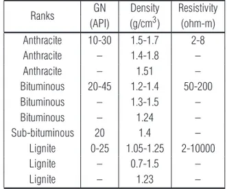
Several geophysical logs can be used to identify coal, estab-lish the rank, and determine the ash content (Hearst et al., 2000; Gasper, 2012). Table 1 shows some geophysical responses for different coal ranks.
Table 1 – Values of geophysical logging parameters for coal ranks. Source: Hearst et al. (2000).
Ranks GN Density Resistivity (API) (g/cm3) (ohm-m) Anthracite 10-30 1.5-1.7 2-8 Anthracite – 1.4-1.8 – Anthracite – 1.51 – Bituminous 20-45 1.2-1.4 50-200 Bituminous – 1.3-1.5 – Bituminous – 1.24 – Sub-bituminous 20 1.4 – Lignite 0-25 1.05-1.25 2-10000 Lignite – 0.7-1.5 – Lignite – 1.23 –
Resistivity: A high resistivity has often been used for coal identification. The bituminous coal type has higher resistivity, but lignite and anthracite can show very low values (Reeves, 1981). In fact, the resistivity reading of lignite can decrease drastically in the presence of water (from 104 to 12 ohm-m, when moisture varies from 0.1 to 0.6). Thus, resistivity must be used with cau-tion due to its wide range of variacau-tion. Besides, some other rock types such as limestone or resistive sandstones also show high-resistivity log deflections in coal-bearing sequences and may be mistaken for coal.
Natural gamma (NG): Most coals contain little or no potas-sium (K40) or thorium (Th232), which makes the values for NG
readings very low. However, some coals have significant quan-tities of uranium (U238/235), producing abnormally high NG
read-ings. Thus, while a low NG is a good indicator for coal and a great way to distinguish between intermediately positioned shales, it is noteworthy that a high value range of NG does not necessarily in-dicate the absence of coal. However, it should also be noted that all four probes utilized in this study have a combined NG features in them. Interestingly, the NG log responses from each are very similar in the same borehole, and consequently only one of them was used for comparisons with the galvanic resistivity logs.
Resistivity Probes used in Data Collection
According to Hearst et al. (2000), guard log (GL) and single-point resistance (SPR) probes are referred to as galvanic resis-tivity tools, which respond to the flow of electric current between the sonde and the strata.
Induction devices (Ellis & Singer, 2007) produce an alternat-ing magnetic field to induce electrical currents in the strata, whose intensity is proportional to the strata’s conductivity. The magni-tude of the induced currents is measured by a tool that senses the magnetic field generated by them.
The GL and induction (IND) log measure the resistivity of the strata, while SPR is an array used to measure the electric resis-tance between the probe and a grounded reference electrode. In this way, the ohm-m is the unit of measurement for the guard and IND probes; the ohm is the unit of measurement for SPR.
GL and SPR need uncased water-filled boreholes, while IND can be run in dry or water-filled, open or plastic-cased boreholes (not steel-cased holes).
Guyod (1944) and Hoffman et al. (1982) describe the theory, use, and general aspects of the design of the SPR tool, which is considered an old tool, although it is still produced by several slimhole manufacturers nowadays. The limitations of this tool are related to the influence of fluid: the resistance of both the bore-hole fluid and the strata contributes to the recorded response, but drilling fluids, which lie closest to the current-electrode, strongly influence the tool’s response. Besides this fact, the measurement of SPR is not made within a definable volume of strata, and thus no quantitative interpretation of resistivity is possible. The response of the SPR tool is nonlinear and tends to emphasize the response of low-resistance seams and compress high-resistance values.
The vertical resolution of SPR in a homogeneous medium is the same as the depth of investigation and approximately five times the diameter of the current-electrode.
General information about GLs and their use is given in Hoff-man et al. (1982) and Ellis & Singer (2007). The GL is a focused resistivity tool, also referred to as a LL3 tool due to its specific array of electrodes. This probe includes three main electrodes: a centrally positioned short current-electrode and two long focusing electrodes positioned laterally with respect to the first. This design has important advantages: the disc-shaped volume of investiga-tion of the tool can be precisely determined while a large depth of investigation and good vertical resolution are achieved. The GL tool is considered to measure the true resistivity of strata rather than the apparent resistivity, as within a small-diameter borehole the amount of borehole fluid is very small and its contribution to the recorded response is usually negligible. The GL array is use-ful for detailed lithologic investigation because its good vertical resolution allows determination of resistivity values for small coal seams. The length of the central current electrode defines the ver-tical resolution of this tool, which can allow a full resolution of coal seams as thin as 5 cm.
According to Monier-Williams et al. (2009), IND logs mea-sure the electrical conductivity and/or magnetic susceptibility of strata using electromagnetic induction. Conductivity is the math-ematical reciprocal of resistivity (measured by galvanic logs). In a two-coil IND logging tool, an electromagnetic field produced by a transmitting coil induces eddy currents, which flow in conductive materials surrounding the borehole. In turn, these eddy currents generate secondary electromagnetic fields, which induce voltages in the receiver coil on the tool. Most tools today have additional coils to obtain a focused depth of investigation while reducing the effect of nearby conductive material and causing the response function to peak at a particular distance from the probe. This has the advantage of rendering these tools relatively insensitive to the fluid in the boreholes, thereby reducing the effects of the borehole on the measurement of the strata’s electrical properties. A long re-view of multi-coil IND logs, including design characteristics and data processing, can be seen in Chapters 7 and 8 of Ellis & Singer (2007). The depth of investigation and vertical resolution are specific for each probe model. In the present work, a seven-coil array tool that allowed two different investigation depths (deep and shallow) was for in data acquisition. No specific details about the coil configuration are present in the tool documentation, and no correction charts for borehole, fluid, and other effects related to the logging tool are available.
The main characteristics of all of the resistivity probes used in data collection are given below:
• SPR: current-electrode diameter = 45 mm; length = 2.70 m; weight = 10 kg.
• GL: diameter = 38 mm; total length = 2.76 m; central cur-rent electrode = 10 cm; length of guard-electrodes = 1 m weight = 8 kg.
• IND log: diameter = 38 m; length = 2.32 m; number of coils = 7; operation frequency = 39 kHz; weight = 8 kg. The ef-fective transmitter-receiving coil spacing is 50 cm for the shallow (ILM) array, and 81 cm for the deep (ILD) array.
METHODOLOGY
The study started by interpreting a set of geophysical logs that were obtained in previous years and also some that were recently logged. The database was however constructed using the follow-ing ideas: any borehole that had geological descriptions and geo-physical logs of at least two of the three probes used in this study (GL, SPR, and IND) was chosen from an existing database in or-der to allow comparisons in each situation. The recent boreholes
permit the collection of geophysical log data with the resistivity probes and optical televiewer (OPTV) probe. The OPTV probe is a geophysical imaging tool that can generate a 360◦ real image of a borehole, which can serve as a digital core sample, provid-ing a direct view of the coal strata in a borehole (an alternative to coring) with higher vertical resolution. However, its use presents some challenges, described later, which must be resolved before its application. For this reason, some operational tests were car-ried out, some of which will be briefly mentioned in the text.
Execution Method Adopted for Data Collection
As previously mentioned, the geophysical logging was carried out in several cored boreholes and blastholes (all vertical) with different depths in various campaigns. The sequence used for geophysical execution during data collection is one of the solu-tions adopted in resolving some of the challenges of the use of OPTV. The execution sequence can be one of the following, as appropriate:
(1) Borehole with fluid: the OPTV probe is executed first, followed by the other probes.
(2) Borehole without fluid (air): there is no specific order of execution.
The reason OPTV is executed first is that there are some con-ditions that must be met to enable it function appropriately. The borehole to be logged must be in favorable conditions to cap-ture a good image. However, in this study, the normal borehole fluid was turbid. This implies that the boreholes must be treated to have a transparent fluid, as stated by Morin (2005), or should be dry (aired). Thus, it became necessary to add a flocculant (aluminum sulfate) several hours before the commencement of geophysical logging. In addition, the work aimed to decant all particulate material and to have clear/transparent fluid inside the borehole at the time of execution of the OPTV. Technically, this substance can be replaced by ferric sulfate and/or ferric chloride (with lower cost) and the same efficiency is guaranteed (Libˆanio et al., 1997; Silva & Lauria, 2006). In regard this, if another probe is executed first, it will definitely disturb the settled particles in the borehole.
Conversely, if OPTV is to be used in dry boreholes, then it is necessary to inject water into these boreholes after its execu-tion before the GL and SPR galvanic probes are executed. The IND probe allows logging with or without fluid.
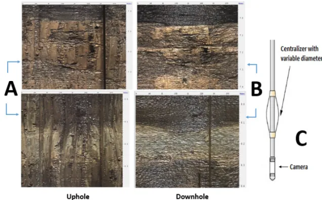
It is important to note that OPTV can be executed either downhole or uphole. The resistivity probes are generally logged
Figure 1 – Illustrative images of geophysical well logging execution using OPTV: (A) uphole, (B) downhole, and (C) schematic illustration of the OPTV probe. Drops of dirt on the glass of the OPTV camera generated the dark vertical lines, as the images were obtained in a dry hole. All in linear scale.
uphole. The uphole execution of OPTV presents drawbacks: the centralizers (Fig. 1C) attached to the probe leave marks on the borehole wall, as seen in both images in Figure 1A impairing the image visual of the wall. In Figure 1B, this effect does not appear, because the images were captured downhole before the centraliz-ers marked the wall.
Identification of Coal Seams using Geophysical Logs
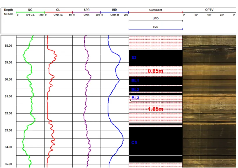
To identify the coal beds in each mineral deposit, a comparison between the recovered core samples and the intervals of the sup-posedly identified coal layers on the geophysical log was con-ducted. That is, in the case of resistivity, NG, and OPTV, as used in this study, coal is identified by high and low signal readings for resistivity and NG in the logs, respectively, whereas in the case of OPTV, the coal is identified by its dark color in the image pro-duced, because it is a dark substance in nature (see Fig. 2 for real illustrations of all involved logs).
In the geophysical logs, to determine the top and base of a coal seam and other materials around it, one can adopt any of several possible methods, as described in Chapter 11 of Hoffman et al. (1982). Here, the procedure used is referred to as the ra-tio method, which was empirically developed by the observara-tion of the resistivity log responses. It is noteworthy that it is best to use two or more geophysical parameter measures (i.e. resistivity, NG, and OPTV, as in this study) for lithology identification, but
the procedure here considers only the coal beds clearly identified by the resistivity logs. With the introduction of the OPTV probe, the challenges faced in determining the top and base of the coal seams are closer to being resolved. Figure 2 shows an example of the complete comparative analysis model involving all geophysi-cal probes used in this study.
In this particular study, only the ILM array (shallow response) of the IND log was used to identify the coal seams, due to its better vertical resolution compared with the ILD array.
DATA ANALYSIS
In this part, the analyzed borehole data from each campaign are presented. Comparisons were made between the thicknesses of coal beds obtained from core sample analysis and those obtained by geophysical readings, in order to detect and determine the es-timated thicknesses of coal beds based on the resistivity contrast provided by these beds.
B3 Campaign
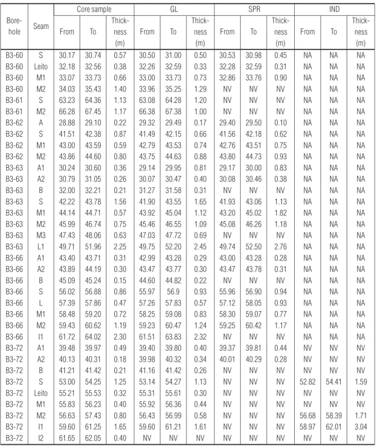
In this campaign, six boreholes were analyzed. Five of them were logged with two resistivity probes while only one has three probes logged (B3-72), as shown in Table 2. The diameter of these boreholes is 75 mm (all the diamond drilling boreholes in this work have the same diameter) and they are fluid-filled. Table 2 shows the coal seams and the respective geophysical
Figure 2 – A complete comparative analysis model adopted for this study (SVN-37). All in linear scale.
probes utilized in each borehole. It also presents comparisons between the thicknesses of coal seams estimated via geophysi-cal reading and by core sample analysis.
Figure 3 presents some analyses from borehole B3-60 in campaign B3. In terms of identification of coal seams, it should be noted that GL was able to identify all three coal seams (Leito, M1, and M2) while SPR only partially identified M2 in the log and this seam was classified as not visible. On the other hand, the small table on the right side of Figure 3 shows that the estimated coal bed thickness produced by GL is closest to that provided by geological logging (note that M2 is overestimated by SPR).
Cerro Campaign
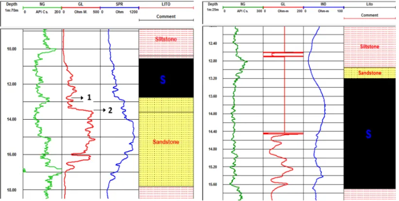
In the Cerro campaign, three boreholes were analyzed. CRN-72 was logged with GL and IND probes while GL and SPR were used for the others. This coal deposit contains sandstone layers, which are a well-known lithology with resistivity and NG readings very similar to coal. Generally, sandstone shows high resistivity and low NG readings too. Notably, for this reason, it is usually confused with coal in the absence of recovered core samples or image generating tools (i.e. OPTV). In cases where there is a
di-rect transitional contact between the coal and sandstone, it may be difficult to discriminate the top and base for each rock type. Figure 4 (left) highlights a typical problem in discrimination be-tween coal and sandstone in the absence of recovered sample. It illustrates a difficult situation in identifying the base of the coal seam and the top of the sandstone, between arrows 1 and 2 (which log is correct?).
Figure 4 (right) illustrates the effect of the absence of fluid from the top of borehole CRN-72 to about 14.5 m on the resis-tivity log of the GL. However, on the other log, this situation has no effect on the IND log, as it can function perfectly in any condi-tion of the borehole, whether dry (air-filled) or fluid-filled. Table 3 presents the thicknesses of the coal seams geologically examined and defined by the probes used in each borehole of the deposit. Additionally, there is a comparison between the estimated thick-nesses of the coal seams obtained from geophysical readings.
Calombo Campaign
The use of OPTV and analysis of its results are the main topic derived from this campaign. In this deposit, two boreholes were logged: CAL-58B and CAL-57. Interestingly, in CAL-58B there
Table 2 – Coal seams of boreholes in Area B3 and the estimated coal thickness defined by geological description and resistivity readings. NA = resistivity log not available; NV = lithological contact not visible.
Bore-Seam
Core sample GL SPR IND
hole From To Thick-From To Thick-From To Thick-From To
Thick-ness ness ness ness
(m) (m) (m) (m) B3-60 S 30.17 30.74 0.57 30.50 31.00 0.50 30.53 30.98 0.45 NA NA NA B3-60 Leito 32.18 32.56 0.38 32.26 32.59 0.33 32.28 32.59 0.31 NA NA NA B3-60 M1 33.07 33.73 0.66 33.00 33.73 0.73 32.86 33.76 0.90 NA NA NA B3-60 M2 34.03 35.43 1.40 33.96 35.25 1.29 NV NV NV NA NA NA B3-61 S 63.23 64.36 1.13 63.08 64.28 1.20 NV NV NV NA NA NA B3-61 M2 66.28 67.45 1.17 66.38 67.38 1.00 NV NV NV NA NA NA B3-62 A 28.88 29.10 0.22 29.32 29.49 0.17 29.40 29.50 0.10 NA NA NA B3-62 S 41.51 42.38 0.87 41.49 42.15 0.66 41.56 42.18 0.62 NA NA NA B3-62 M1 43.00 43.59 0.59 42.79 43.53 0.74 42.76 43.51 0.75 NA NA NA B3-62 M2 43.86 44.60 0.80 43.75 44.63 0.88 43.80 44.73 0.93 NA NA NA B3-63 A1 30.24 30.60 0.36 29.14 29.95 0.81 29.17 30.00 0.83 NA NA NA B3-63 A2 30.79 31.05 0.26 30.07 30.47 0.40 30.08 30.46 0.38 NA NA NA B3-63 B 32.00 32.21 0.21 31.27 31.58 0.31 NV NV NV NA NA NA B3-63 S 42.22 43.78 1.56 41.90 43.55 1.65 41.93 43.06 1.13 NA NA NA B3-63 M1 44.14 44.71 0.57 43.92 45.04 1.12 43.20 45.02 1.82 NA NA NA B3-63 M2 45.99 46.74 0.75 45.46 46.55 1.09 45.08 46.26 1.18 NA NA NA B3-63 M3 47.43 48.06 0.63 47.03 47.72 0.69 NV NV NV NA NA NA B3-63 L1 49.71 51.96 2.25 49.75 52.20 2.45 49.74 52.50 2.76 NA NA NA B3-66 A1 43.40 43.71 0.31 42.99 43.28 0.29 43.00 43.28 0.28 NA NA NA B3-66 A2 43.89 44.19 0.30 43.47 43.77 0.30 43.47 43.78 0.31 NA NA NA B3-66 B 45.09 45.24 0.15 44.60 44.82 0.22 NV NV NV NA NA NA B3-66 S 56.02 56.88 0.86 55.97 56.9 0.93 55.96 56.90 0.94 NA NA NA B3-66 L 57.39 57.86 0.47 57.26 57.83 0.57 57.12 58.05 0.93 NA NA NA B3-66 M1 58.48 59.20 0.72 58.25 59.08 0.83 58.30 59.07 0.77 NA NA NA B3-66 M2 59.43 60.62 1.19 59.23 60.47 1.24 59.25 60.42 1.17 NA NA NA B3-66 I1 61.72 64.02 2.30 61.51 63.83 2.32 NV NV NV NA NA NA B3-72 A1 39.48 39.97 0.49 39.40 39.80 0.40 39.37 39.81 0.44 NV NV NV B3-72 A2 40.13 40.31 0.18 39.98 40.32 0.34 40.01 40.29 0.28 NV NV NV B3-72 B 41.21 41.42 0.21 41.16 41.42 0.26 NV NV NV NV NV NV B3-72 S 53.00 54.25 1.25 53.14 54.27 1.13 NV NV NV 52.82 54.41 1.59 B3-72 Leito 55.21 55.53 0.32 55.31 55.61 0.30 NV NV NV NV NV NV B3-72 M1 55.83 56.23 0.40 55.92 56.36 0.44 NV NV NV NV NV NV B3-72 M2 56.63 57.43 0.80 56.43 56.99 0.58 NV NV NV 56.68 58.39 1.71 B3-72 I1 59.60 61.25 1.65 59.60 61.21 1.61 NV NV NV 58.97 62.01 3.04 B3-72 I2 61.65 62.05 0.40 NV NV NV NV NV NV NV NV NV
was an occurrence of fluid escaping from the borehole due to a mechanical fracture. However, it was discovered from the OPTV images that the borehole could only hold water at the depth of ap-proximately 40.9 m (Fig. 5). Such a situation resulted in the use of only the IND probe for data collection. This is a special situation
in which data collection and obtaining geophysical readings were possible in a single borehole that was dry and fluid-filled at the same time. Extreme right image of Figure 5 shows a real image of transition from dry to water in the borehole.
Figure 3 – Comparisons of resistivity logs (GL and SPR) along with the geological core sample in borehole B3-60 and, on the right side, the thicknesses of coal seams estimated using resistivity logs (GL and SPR) and the recovered core sample in borehole B3-60. All in linear scale.
Figure 4 – Images showing the transitional contact of coal and sandstone (left) and the effect of the absence of fluid (right) in boreholes CRN-82 and CRN-72, respectively. All in linear scale.
and was used as one of the OPTV operational tests. The OPTV was unable to register any visual of the borehole wall without the addition of flocculant to the borehole water.
Seival Campaign
In this area, only one borehole (SVN-37) was analyzed and it was the only borehole where all the probes (GL, SPR, IND, and OPTV)
used in this study were executed, including the addition of floc-culant to the borehole fluid. Part of the obtained register of each probe in this particular borehole is shown in Figure 6.
It is important to state here that the presence of conductive fluid (effect of aluminum sulfate) had an impact on the resistivity logs. The full identification of the coal seams by the geophysical method and by geological description is shown in Table 4).
Table 3 – Coal seams of boreholes in the Cerro campaign and the estimated coal thicknesses defined by geological description and resistivity readings. NA = resistivity log not available; NV = lithological contact not visible.
Borehole Steam
Core sample GL SPR IND Thickness Thickness Thickness Thickness
(m) (m) (m) (m) CRN-72 S 2.50 NA NA 2.52 CRN-72 M2 1.20 NA NA 0.70 CRN-72 M3 0.11 NA NA NV CRN-81 S 2.10 2.25 2.32 NA CRN-81 M1 0.45 0.44 0.44 NA CRN-81 M2 1.40 1.45 1.89 NA CRN-82 S 2.20 2.38 1.76 NA CRN-82 M1 0.60 0.69 0.75 NA CRN-82 M2 1.40 NV NV NA
Figure 5 – Absence of fluid from the borehole top to 40.9 m and (extreme right) transitional image from dry to fluid in borehole CAL-58. All in linear scale.
RESULTS ANALYSIS
The analysis of geophysical logs allows us to reach an answer regarding the main question raised in this study: which among the three types of resistivity probes is the most appropriate for use in the mentioned coal deposits, considering which one allows easier and clearer visual recognition of the coal strata?
Thus, the following criteria will be used to justify the best choice:
(a) The definition of the probe that identifies the highest number of coal strata in the logged boreholes.
(b) The definition of the probe that presents the smallest dif-ference in coal bed thickness between the geologically de-scribed thickness (core sample) and the thickness deter-mined by geophysical logging.
In the course of the analyses, using criterion (a), the probe that was able to identify the highest number of coal beds was GL. Table 5 shows the results obtained after comparing the three probes used in the detection of coal seams.
Using criterion (b), the GL probe proved to be the one that approximated the coal bed thickness most closely. For the sake
Figure 6 – Image of SVN-37 showing a complete comparison of the three resistivity logs plus the OPTV image (A) and the test for the vertical resolution of OPTV when the contact is abrupt and gradual (B and C), respectively. All in linear scale.
Table 4 – Coal seams of borehole SVN-37 in the Seival campaign and the es-timated coal bed thicknesses defined by geological description and geophysical electric logs. NV = lithological contact not visible.
Coal Core sample GL SPR IND Steam Thickness Thickness Thickness Thickness
(m) (m) (m) (m) S5 0.37 NV NV NV S4 1.02 0.93 NV 1.04 S3 1.30 1.21 NV 1.41 S2 0.94 0.89 0.91 1.11 BL1-BL3 1.07 1.09 1.31 1.21 S 2.25 2.29 NV 2.13 L 1.57 1.59 NV 1.56 L1 1.37 1.22 NV 1.08 L2 0.95 0.85 0.85 1.06 L3 0.95 1.16 1.36 1.26 L4 0.60 NV NV NV
of simplification, only two (2) boreholes will be presented here: B3-72 and SVN-37. These boreholes show a complete register of the resistivity probes utilized. Table 6 shows the comparison made considering these two boreholes. In relation to this, it should be noted that using the criterion (b) employed in the analysis of other boreholes cited in this work, the results and conclusion obtained were the same as those shown in Table 5.
CONCLUSIONS
The main objective of this study was to analyze the applicability of three different geophysical probes (GL, SPR, and IND log) for measuring the electrical resistivity in specific coal deposits.
The analysis of geophysical logs obtained in the field, when compared to the geological descriptions (core samples), showed
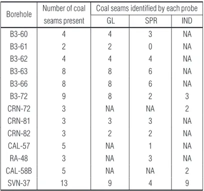
Table 5 – Number of successfully identified coal strata for each resistivity probe (GL, SPR, and IND). NA = geophysical log not available.
Borehole Number of coal Coal seams identified by each probe seams present GL SPR IND
B3-60 4 4 3 NA B3-61 2 2 0 NA B3-62 4 4 4 NA B3-63 8 8 6 NA B3-66 8 8 6 NA B3-72 9 8 2 3 CRN-72 3 NA NA 2 CRN-81 3 3 3 NA CRN-82 3 2 2 NA CAL-57 5 NA 1 NA RA-48 3 NA 3 NA CAL-58B 5 NA NA 2 SVN-37 13 9 4 9
Table 6 – Differences between the thicknesses of coal strata as obtained from geo-physical logs and by geological descriptions. NV = lithological contact not visible.
Borehole Seam
Core Difference in thickness between thickness geological and geophysical logs (m) GL (m) SPR (m) IND (m) B3-72 A1 0.49 0.09 0.05 NV A2 0.18 -0.16 -0.10 NV B 0.21 -0.05 NV NV S 1.25 0.12 NV -0.34 Leito 0.32 0.02 NV NV M1 0.40 -0.04 NV NV M2 0.80 0.22 NV -0.91 I1 1.65 0.04 NV -1.39 I2 0.40 NV NV NV SVN-37 S5 0.37 -0.08 NV NV S4 1.02 0.09 NV -0.02 S3 1.30 0.09 NV -0.11 S2 0.94 0.05 0.03 -0.17 BL1-BL3 1.07 -0.02 -0.24 -0.14 S 2.25 -0.04 NV 0.12 L 1.57 -0.02 NV 0.01 L1 1.37 0.15 NV 0.29 L2 0.95 0.10 0.10 -0.11 L3 0.95 -0.21 -0.41 -0.31 L4 0.60 -0.08 NV NV
that GL presented the most detailed resistivity readings for coal strata in the vast majority of cases. It permits contact discrimi-nation between coal and waste, and even detects coal partings in different situations. Thus, the geophysical estimates of coal seam thickness presented by GL were closer to those provided by the geological description than the estimates presented by the other probes, and GL can identify thin coal beds with thicknesses ex-ceeding about 15 cm.
The IND probe can be qualified as the second-best probe in terms of sensor arrangement, considering the same criteria. How-ever, it can only identify large coal beds with thicknesses exceed-ing 70 cm, as shown in Figure 2. Also, regardexceed-ing vertical reso-lution, IND has a major difficulty in registering partings between coal beds. In contrast, IND has an advantage over other probes in that it is the only probe that can be used in dry (air-filled) bore-holes, as the GL and SPR operations necessarily require a con-ductive fluid in the borehole.
Secondarily, another objective of interest here is to assess whether the images generated by the OPTV probe can improve the detection of coal beds and the vertical resolution of resistiv-ity probes. However, it was observed in the images that when the coal and waste contact is abrupt, OPTV allows coal seams with thicknesses of less than 5 cm to be discriminated. In this situa-tion (abrupt contact), the image obtained by OPTV (Fig. 6B) offers excellent support as a verification tool to enhance the geological description when there are core losses. The images show equal quality to the core directly taken from sample boxes. On the other hand, when the contact is gradual (Fig. 6C), the identification is subject to errors that vary in each situation. Moreover, another drawback of using the OPTV is the time spent in fluid prepara-tion, which is a time-consuming task and can preclude its use in common situations.
Finally, from the conclusions above, some aspects can be highlighted:
• The logs made in the field made it possible to evaluate the viability of these logs in real situations, where all the vari-ability of the lithologies is present.
• It is possible to validate the empirical rules of marking the contacts in real situations without the need for holes pre-pared specifically for this purpose, which would imply time and cost of preparation.
• As there is no detailed information about the coil arrange-ment and data processing in the tool docuarrange-mentation of this specific induction array tested (ILM), so its vertical
resolu-tion is unknown. With the tests conducted in the field it is possible to obtain a good idea of the equipment responses.
REFERENCES
AFONSO JMS. 2014. Electrical resistivity measurementsin coal: assess-ment of coal-bed methane content, reserves and coal permeability. PhD Thesis, Department of Geology, University of Leicester, Leicester, 2014. 272 pp.
BORSARU M & ASFAHANIA J. 2007. Low-activity spectrometric gamma-ray logging technique for delineation of coal/rock interfaces in dry blast holes. Applied Radiation and Isotopes. Amsterdam. vol. 65. 748–755. Jun.
ELLIS DV & SINGER JM. 2007. Well logging for earth scientists. 2nd ed., Springer-Verlag, New York, 692 pp.
FIRTH D. 1999. Log Analysis for Mining Applications. Ed. Elkington P. Reeves Wireline Services, Brendale, 164 pp.
GASPER GO. 2012. Estimativa de qualidade de carv˜ao a partir de perfi-lagem geof´ısica e seu uso no planejamento de lavra a curto prazo. Mas-ter Dissertation – Programa de P´os-Graduac¸˜ao em Engenharia de Minas, Metal´urgica e de Materiais. Universidade Federal do Rio Grande do Sul, Brazil. 2012. 89 pp.
GUYOD H. 1944. The single-point resistance method. Oil Weekly, vol. 114, n. 12, Aug. 21, 1944.
HEARST JR, NELSON PH & PAILLET FL. 2000. Well logging for physical properties. 2nd ed., John Wiley & Sons, New Jersey. 483 pp.
HOFFMAN GL, JORDAN GR & WALLIS GR. 1982. Geophysical bore-hole logging handbook for coal exploration. The Coal Mining Research Centre, Edmonton. 270 pp.
KAYAL JR. 1979. Electrical and gamma-ray logging in Gondwana and Tertiary coalfields of India. Geology and Exploration, 17: 243–258. KAYAL JR & CHRISTOFFEL DA. 1989. Coal quality from geophysical logs: Southland lignite region, New Zealand. The Log Analyst, 30: 343– 352.
LIBˆANIO M, PEREIRA MM, VORCARO BM, RAIMUNDA CR & HELLER L. 1997. Avaliac¸˜ao do Emprego de Sulfato de Alum´ınio e do Cloreto F´errico na Coagulac¸˜ao de ´Agua Naturais de Turbidez M´edia e Cor Ele-vada. In: Feira Internacional de Tecnologias de Saneamento Ambiental. Rio de Janeiro. Anais: Associac¸˜ao Brasileira de Engenharia Sanit´aria e Ambiental (ABES), 1365–1373.
MONIER-WILLIAMS ME, DAVIS RK, PAILLET FL, TURPENING RM, SOL SJY & SCHNEIDER GW. 2009. Review of borehole based geophys-ical site evaluation tools and techniques. NWMO TR-2009-25 Report. Golder Associates, University of Arkansas, Michigan Technical Univer-sity, November.
MORIN RH. 2005. Hydrologic properties of coal beds in the Powder River Basin. Montana I: Geophysical log analysis. Journal of Hydrology, Amsterdam, 308(1-4): 227–241 (Jul).
REEVES DR. 1981. Coal interpretation manual. BPB Instruments, East Lake, 100 pp.
SILVA CNF & LAURIA RG. 2006. Estudo da Viabilidade T´ecnica e Eco-nˆomica da Substituic¸˜ao do Sulfato de Alum´ınio pelo Cloreto F´errico ou Sulfato F´errico no Tratamento de ´Agua de Abastecimento. Undergradu-ate Final Project. Civil Engineering. Fundac¸˜ao Educacional de Barretos, Barretos, Brazil. 126 pp.
Recebido em 8 junho, 2017 / Aceito em 8 dezembro, 2017 Received on June 8, 2017 / Accepted on December 8, 2017