Quadrature Generators based on Ring Oscillators and Shift Registers

Licenciado em Ciências da Engenharia Eletrotécnica e de Computadores

Quadrature Generators based on Ring

Oscillators and Shift Registers

Dissertação para obtenção do Grau de Mestre em Engenharia Eletrotécnica e de Computadores

Orientador: Prof. Dr. Luís Augusto Bica Gomes de Oliveira, Prof. Auxiliar, Universidade Nova de Lisboa

Júri:

Presidente: Prof. Dr. Luís Filipe Figueira de Brito Palma Arguente: Prof. Dr. Rui Manuel Leitão Santos Tavares

Copyright © João Pedro Costa Pinto, Faculty of Sciences and Technology, Nova University of Lisbon

I would like to address a special appreciation to the Faculty of Sciences and Technol-ogy of Nova University of Lisbon, namely the Department of Electrical Engineering by how welcomed me since I joined the higher education, so that I can say after this journey this institute was undoubtedly a second home to me.

I am very grateful not only for the learning conditions available under consistent and friendly guidance on a healthy working environment, but also for the people I had the pleasure to know and those I’ll take with me from now on.

One of these persons is my professor and advisor Professor Luís Oliveira, which proved to be always available to assist me with all his commitment and enthusiasm that best characterize him, never underestimating his solid knowledge concerning the context of my dissertation and everything it covers. I cannot express how grateful I am for his huge eff_{ort and encouragement through the development of the thesis. My most sincere thanks.}

I would like to mention Eduardo Ortigueira and Miguel Fernandes and thank them for their help, guidance and patience provided during this project.

Those who followed the whole course of this project were my cabinet colleagues, to whom I owe a special thanks for the fellowship, good atmosphere and for every single advice they gave me targeting the improvements my work could suff_er.

No less important was the role of my family, particularly my parents and uncles Miguel and Lídia, the aff_{ection that has been noted throughout my life and during my} academic path, the freedom they always gave me and for have always supported in any and every decision that I have made. Without them I certainly couldn’t reach where I reached today and for that reason thank you for being always a source of love, support and encouragement.

Finally, I want to thank one of the most important cornerstones of my life: my dear girlfriend Ana Rita Moital for her endless love, patience and understanding.

Last but not least, to my childhood friends, though they are not mentioned here, somehow had their contribution to the person I am today and have always been with me in the good and bad moments.

Quadrature oscillators are key elements in modern radio frequency (RF) transceivers and very useful nowadays in wireless communications, since they can provide: low quadrature error, low phase-noise, and wide tuning range (useful to cover several bands). RC oscillators can be fully integrated without the need of external components (external highQ-inductors), optimizing area, cost, and power consumption.

The conventional structure of ring oscillator off_{ers poor frequency stability and} phase-noise, low quality factor (Q), and besides being vulnerable to process, voltage and temper-ature (PVT) variations, its performance degrades as the frequency of operation increases. This thesis is devoted to quadrature oscillators and presents a detailed comparative study of ring oscillator and shift register (SR) approaches. It is shown that in SRs both phase-noise and phase error are reduced, while ring oscillators have the advantage of occupying less area and less consumption due to the reduced number of components in the circuit. Thus, although ring oscillators are more suitable for biomedical applica-tions, SRs are more appropriate for wireless applicaapplica-tions, especially when specification requirements are more stringent and demanding.

The first architecture studied consists in a simple CMOS ring oscillator employing an odd number of static single-ended inverters as delay cells. Subsequently, the quadra-ture 4-stage ring oscillator concept is shown and post-layout simulations are presented. The 3 and 4-phase single-frequency local oscillator (LO) generators employing SRs are presented, the latter with 50% and 25% duty-cycles. The circuits operate at 600 MHz and 900 MHz, and were designed in a 130 nm standard CMOS technology with a voltage supply of 1.2 V.

Os osciladores em quadratura são elementos fulcrais no que concerne aos mais re-centes transceivers de rádio frequência (RF) e às comunicações sem fio de hoje em dia sobretudo graças às mais-valias que ostentam: baixos erro de quadratura e ruído de fase e ampla faixa de sintonização (útil para cobrir diversas bandas). Os osciladores RC podem ser totalmente integrados sem a necessidade de recorrer a componentes externos (indu-tores externos com elevado fator de qualidade [Q]), otimizando assim a área, custo e o consumo associados.

A estrutura convencional do oscilador em anel a par de uma pobre estabilidade de frequência e ruído de fase, apresenta um baixo fator de qualidade e além de ser vulne-rável a variações de processo, tensão e temperatura (PVT do inglêsprocess, voltage and temperature), o seu desempenho diminui à medida que a frequência de operação aumenta.

Esta tese é dedicada aos osciladores em quadratura, apresentando um detalhado es-tudo comparativo dos osciladores em anel e shift registers (SRs). Tanto o ruído de fase como o erro de fase são reduzidos nos SRs, ao passo que o oscilador em anel tem a van-tagem de ocupar menos área e apresentar menor consumo, graças ao modesto número de componentes que possui. Assim, embora os osciladores em anel sejam mais adequa-dos para aplicações biomédicas, os SRs são mais apropriaadequa-dos para aplicações wireless, sobretudo quando as especificações são mais rigorosas e exigentes.

A primeira topologia estudada consiste num simples oscilador em anel CMOS empre-gando um número ímpar de inversores como células de atraso. Posteriormente, o oscilador em anel de 4 estágios em quadratura é apresentado, bem como simulações pós-layout do mesmo. Relativamente aos SRs, desenvolveu-se geradores de 3 e 4 fases onde a arqui-tetura em causa é aplicada, o último com duty-cyclesde 50% e 25%. Todos os circuitos operam a 600 MHz e 900 MHz e foram desenvolvidos na tecnologia padrão CMOS de 130 nm com uma tensão de alimentação de 1,2 V.

List of Figures xvii

List of Tables xxi

1 Introduction 1

1.1 Background and Motivation . . . 1

1.2 Main Contributions . . . 4

1.3 Thesis Outline . . . 5

2 Transceiver Architectures 7 2.1 Receiver Architectures . . . 7

2.1.1 Heterodyne Receiver . . . 8

2.1.2 Homodyne Receiver . . . 9

2.1.3 Low-IF Receiver . . . 11

2.2 Transmitter Architectures . . . 12

2.2.1 Heterodyne Transmitters . . . 13

2.2.2 Direct Upconversion Transmitter . . . 14

3 Oscillators 15 3.1 Basic Concepts . . . 16

3.1.1 Performance . . . 16

3.1.2 MOS Transistor Overview . . . 18

3.1.3 Noise . . . 24

3.2 Oscillator Basic Concepts . . . 27

3.2.1 Barkhausen Stability Criterion . . . 27

3.2.2 Quality Factor . . . 28

3.2.3 Phase-noise . . . 31

3.2.4 Figure of Merit . . . 35

3.3 Single Oscillator Topologies . . . 36

3.3.1 LC Oscillator . . . 36

3.3.2 RC Oscillator . . . 39

4.1 Closed-loop Approaches . . . 50

4.1.1 Two-Integrator Oscillator . . . 50

4.1.2 Coupled Oscillators . . . 55

4.2 Open-loop Approaches . . . 58

4.2.1 RC All-pass Filter . . . 58

4.2.2 RC Polyphase Filter . . . 61

4.2.3 Frequency Divide-by-two Circuits . . . 62

4.2.4 Shift Register . . . 62

5 Analysis of Multiphase Generators 71 5.1 Multiphase Ring Oscillators . . . 71

5.1.1 3-stage Ring Oscillator . . . 71

5.1.2 4-stage Ring Oscillator . . . 75

5.2 Multiphase Shift Registers . . . 76

5.2.1 3-phase Shift Register . . . 76

5.2.2 4-phase Shift Register with 50% Duty-cycle . . . 78

5.2.3 4-phase Shift Register with 25% Duty-cycle . . . 79

6 Simulation Results 81 6.1 Schematic Simulations . . . 82

6.1.1 3-stage Ring Oscillator . . . 82

6.1.2 3-phase Shift Register . . . 86

6.1.3 4-stage Ring Oscillator . . . 90

6.1.4 4-phase Shift Register with 50% Duty-cycle . . . 94

6.1.5 4-phase Shift Register with 25% Duty-cycle . . . 97

6.2 Layout Design . . . 101

6.2.1 Layout Considerations . . . 101

6.2.2 Hierarchical Layout . . . 103

6.3 Post-layout Simulations . . . 112

6.3.1 4-stage Ring Oscillator . . . 112

6.4 Analysis of Results and Discussion . . . 115

7 Conclusion and Future Work 119 7.1 Conclusion . . . 119

7.2 Future Work . . . 120

Bibliography 123 A Performance of the Individual Blocks 135 A.1 CMOS Inverter . . . 136

A.2 AND Logic Gate . . . 136

A.4 Single D-FF . . . 138

A.5 Dual D-FF . . . 139

B Simulations Description 141 B.1 DC Analysis . . . 142

B.2 Transient Analysis . . . 142

B.3 PSS Analysis . . . 143

B.4 Pnoise Analysis . . . 143

B.5 Monte Carlo Analysis . . . 144

1.1 Wireless system block diagram . . . 2

2.1 Superheterodyne receiver . . . 8

2.2 Image signal in superheterodyne receiver . . . 9

2.3 Homodyne receiver . . . 10

2.4 Image rejection architectures . . . 12

2.5 Heterodyne transmitter . . . 13

2.6 Direct upconversion transmitter . . . 14

3.1 Classification of oscillators . . . 16

3.2 Definition of propagation delays and rise and fall times . . . 17

3.3 50%, 75% and 25% duty-cycle examples . . . 18

3.4 Simplified MOS transistor incremental scheme . . . 19

3.5 MOS capacitances . . . 20

3.6 MOS high-frequency small-signal model . . . 21

3.7 Small-signal model for a MOS transistor in the saturation region . . . 21

3.8 Cross section of a MOS operating in the saturation region . . . 22

3.9 Distributed RC model for a transistor in the triode region . . . 23

3.10 Simplified triode-region model valid for smallVDS . . . 23

3.11 Small-signal model for a MOS that is turned off _{. . . . 24}

3.12 Types of noise . . . 25

3.13 Power spectrum of flicker and thermal noise . . . 27

3.14 Basic oscillator configuration . . . 27

3.15 BPF frequency response and BPFQfactor . . . 30

3.16 Definition ofQbased on open-loop phase slope . . . 30

3.17 Output waveforms of an ideal and a noisy oscillator . . . 31

3.18 Spectrum of oscillator output with phase-noise . . . 32

3.19 A typical asymptotic noise spectrum at the oscillator output . . . 33

3.20 Phase-noise eff_{ect on RF systems . . . . 34}

3.21 Phase-noise eff_{ect on the receiver and the undesired downconversion . . . . 35}

3.22 Phase-noise eff_{ect on the transmitter path . . . . 35}

3.23 LC-oscillator behavioural model . . . 37

3.25 Small-signal model of the diff_{erential pair . . . . 38}

3.26 A conventional relaxation oscillator . . . 40

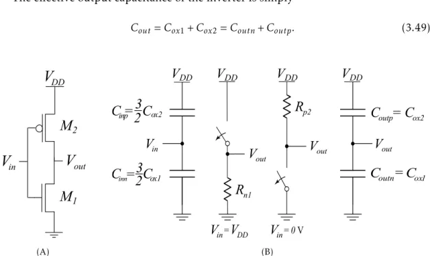
3.27 CMOS inverter switching characteristics using the digital model . . . 41

3.28 Dynamic power dissipation of the CMOS inverter . . . 43

3.29 Voltage-transfer characteristic of the CMOS inverter . . . 43

3.30 Small-signal model of the CMOS inverter . . . 44

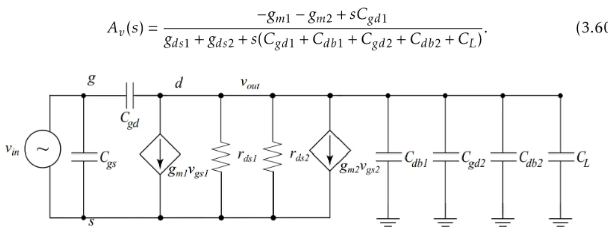
3.31 Simplified small-signal model of the CMOS inverter . . . 44

3.32 High-frequency small-signal model of the CMOS inverter . . . 44

3.33 Ring oscillator withN delay stages . . . 45

3.34 Linear model of an idealN-stage (N≥3) ring oscillator . . . 46

4.1 High level study of two-integrator oscillator . . . 50

4.2 Two-integrator oscillator implementation . . . 51

4.3 Current flow in the two-integrator oscillator circuit . . . 52

4.4 Two-integrator oscillator high level model with non-linear behaviour . . . . 52

4.5 Two-integrator oscillator high level model with linear behaviour . . . 53

4.6 Small-signal model of diff_{erential pair composed of transistorsMr . . . . 53}

4.7 Small-signal analysis of transconductance . . . 54

4.8 Two-integrator oscillator linear model . . . 54

4.9 Coupled LC oscillator circuit . . . 56

4.10 Coupled RC oscillator high level model . . . 57

4.11 Coupled RC oscillator circuit . . . 57

4.12 RC all-pass phase shifter diagram . . . 59

4.13 RC-CR circuit as a quadrature generator . . . 60

4.14 RC polyphase network as a symmetric RC network . . . 61

4.15 Quadrature generation using a divide-by-two circuit . . . 62

4.16 Classification of logic circuits based on their temporal behaviour . . . 63

4.17 Latch and flip-flop timing diagrams . . . 64

4.18 Shift register data movement . . . 65

4.19 5-bit SISO shift register . . . 66

4.20 Data bits stored after five clock pulses . . . 67

5.1 CMOS inverter circuit . . . 72

5.2 3-stage single-ended ring oscillator . . . 73

5.3 Quadrature 4-stage ring oscillator concept employing feedforward paths . . 76

5.4 2-input NAND gate and single D flip-flop structure . . . 77

5.5 Dual D flip-flop structure . . . 78

5.6 3-phase shift register block diagram . . . 78

5.7 Quadrature 4-phase shift register with 50% duty-cycle . . . 78

5.8 2-input AND gate using MOSFET transistors . . . 79

6.1 Oscillator transient response (fLO= 600 MHz) . . . 83

6.2 Oscillator phase-noise (fLO= 600 MHz) . . . 84

6.3 Phase error histogram (µ= 0.7255°,σ= 9.27°) . . . 84

6.4 Oscillator transient response (fLO= 900 MHz) . . . 85

6.5 Oscillator phase-noise (fLO= 900 MHz) . . . 86

6.6 Phase error histogram (µ= 0.0074°,σ= 0.11°) . . . 86

6.7 Generator transient response (fLO= 600 MHz) . . . 87

6.8 Generator phase-noise (fLO= 600 MHz) . . . 88

6.9 Phase error histogram (µ= 0.0002°,σ= 0.03°) . . . 88

6.10 Generator transient response (fLO= 900 MHz) . . . 89

6.11 Generator phase-noise (fLO= 900 MHz) . . . 89

6.12 Phase error histogram (µ= 0.0008°,σ= 0.05°) . . . 90

6.13 Oscillator transient response (fLO= 600 MHz) . . . 91

6.14 Oscillator phase-noise (fLO= 600 MHz) . . . 91

6.15 Phase error histogram (µ= 0.0056°,σ= 0.62°) . . . 92

6.16 Oscillator transient response (fLO= 900 MHz) . . . 93

6.17 Oscillator phase-noise (f_LO= 900 MHz) . . . 93

6.18 Phase error histogram (µ= 0.0086°,σ= 0.47°) . . . 94

6.19 Generator transient response (fLO= 600 MHz) . . . 95

6.20 Generator phase-noise (f_LO= 600 MHz) . . . 95

6.21 Phase error histogram (µ= 0.0010°,σ= 0.03°) . . . 96

6.22 Generator transient response (fLO= 900 MHz) . . . 96

6.23 Generator phase-noise (f_LO= 900 MHz) . . . 97

6.24 Phase error histogram (µ= 0.0012°,σ= 0.06°) . . . 97

6.25 Generator transient response (fLO= 600 MHz) . . . 98

6.26 Generator phase-noise (f_LO= 600 MHz) . . . 99

6.27 Phase error histogram (µ= 0.0011°,σ= 0.04°) . . . 99

6.28 Generator transient response (fLO= 900 MHz) . . . 100

6.29 Generator phase-noise (f_LO= 900 MHz) . . . 100

6.30 Phase error histogram (µ= 0.0019°,σ= 0.06°) . . . 101

6.31 Layout of the 1.2V Twin well RF NMOS used . . . 103

6.32 Subcircuit topology of 1.2V Twin Well RF NMOS . . . 104

6.33 Layout of the 1.2V RF PMOS used . . . 105

6.34 Subcircuit topology of 1.2V RF PMOS . . . 105

6.35 Layout of the MIM capacitor used . . . 106

6.36 Layout of MIMCAPS_MML_130E and MIMCAPS_RF capacitors respectively side by side . . . 107

6.37 Layout of the designed CMOS inverter . . . 108

6.38 Oscillator core and buff_{er schematic . . . . 109}

6.39 Layout of the designed oscillator core and buff_{er . . . . 109}

6.41 Layout of the designed 4-stage ring oscillator . . . 111

6.42 Oscillator transient response (fLO= 1.1 GHz) . . . 113

6.43 Oscillator phase-noise (f_LO= 1.1 GHz) . . . 113

6.44 Phase error histogram (µ= 1.1851°,σ= 21.43°) . . . 114

6.45 Oscillator transient response (fLO= 1.6 GHz) . . . 114

6.46 Oscillator phase-noise (f_LO= 1.6 GHz) . . . 115

6.47 Phase error histogram (µ= 0.8702°,σ= 11.56°) . . . 115

A.1 Inverter transient response . . . 136

A.2 AND transient response . . . 137

A.3 NAND transient response . . . 138

A.4 Single D-FF transient response . . . 139

A.5 Dual D-FF transient response . . . 140

4.1 D-type flip-flop truth table . . . 64

4.2 Shifting a 5-bit code into a SISO shift register . . . 66

4.3 Shifting a 5-bit code out of a SISO shift register . . . 67

5.1 Ring oscillators parameters . . . 74

5.2 Shift register parameters . . . 77

5.3 Truth table of the quadrature 4-phase shift register with 25% duty-cycle . . 79

5.4 Parameters of the quadrature 4-phase shift register with 25% duty-cycle . . 80

6.1 CAD tools and corresponding versions used . . . 82

6.2 DC operating point of the 3-stage ring oscillator for a fundamental frequency of 600 MHz . . . 83

6.3 DC operating point of the 3-stage ring oscillator for a fundamental frequency of 900 MHz . . . 85

6.4 DC operating point of the 4-stage ring oscillator for a fundamental frequency of 600 MHz . . . 90

6.5 DC operating point of the 4-stage ring oscillator for a fundamental frequency of 900 MHz . . . 92

6.6 4-stage ring oscillator pre- and post-layout results . . . 116

6.7 Comparison of state-of-the-art RC oscillators . . . 117

6.8 3-phase LO generators parameters . . . 118

6.9 4-phase LO generators parameters . . . 118

6.10 Comparison of LO generators tradeoff_{s . . . . 118}

A.1 Inverter truth table . . . 136

A.2 AND truth table . . . 137

A.3 NAND truth table . . . 138

AC Alternating Current.

ADC Analog-to-Digital Converter.

AFE Analogue Front-End.

AM Amplitude Modulation.

ASCII American Standard Code for Information Interchange.

BER Bit Error Rate.

BPF BandPass Filter.

CAD Computer-Aided Design.

CD Critical Dimension.

CML Current-Mode Logic.

CMOS Complementary Metal-Oxide-Semiconductor.

D-FF D-type FlipFlop.

DC Direct Current.

DDR Double Data Rate.

DLL Delay-Locked Loop.

DRC Design Rule Checking.

DRM Digital Rights Management.

DSP Digital Signal Processing.

DTC Divide-by-Two Circuits.

EDA Electronic Design Automation.

FET Field-Eff_{ect Transistor.}

FF Flip-Flop.

FM Frequency Modulation.

FoM Figure of Merit.

FPGA Field Programmable Gate Array.

GSM Global System for Mobile Communications.

I/O Input/Output.

IC Integrated Circuit.

IF Intermediate Frequency.

IP Intellectual Property.

IP2 Second-order Intercept Point.

ISM Industrial, Scientific and Medical.

L Phase-noise.

LNA Low-Noise Amplifier.

LO Local Oscillator.

LPE Layout Parameter Extraction.

LPF Low-Pass Filter.

LSB Least Significant Bit.

LSI Large-Scale Integration.

LTI Linear Time-Invariant.

LTV Linear Time-Variant.

LVS Layout Versus Schematic.

MIM Metal-Insulator-Metal.

MIMCAP Metal-Insulator-Metal CAPacitor.

MOS Metal-Oxide-Semiconductor.

MOSFET Metal-Oxide-Semiconductor Field-Eff_{ect Transistor.}

ODE Oscillator Design Effi_ciency.

PA Power Amplifier.

PAC Periodic AC.

PDK Process Design Kit.

PIPO Parallel-Input to Parallel-Output.

PISO Parallel-Input to Serial-Output.

PLL Phase-Locked Loop.

PMOS Positive-channel Metal-Oxide-Semiconductor.

Pnoise Periodic Noise.

PSD Power Spectral Density.

PSP Periodic S-Parameter.

PSS Periodic Steady-State.

PVT Process, Voltage and Temperature.

PXF Periodic Transfer Function.

Q Quality Factor.

QAM Quadrature Amplitude Modulation.

QDR Quadrature Data Rate.

QPSK Quadrature Phase-Shift Keying.

RF Radio Frequency.

SIPO Serial-Input to Parallel-Output.

SISO Serial-Input to Serial-Output.

SoC System-on-a-Chip.

SR Shift Register.

SSB Single-SideBand modulation.

TLR Topological Layout Rules.

UMC United Microelectronics Corporation.

VLSI Very-Large-Scale Integration.

C

h

a

p

t

1

I n t r o d u c t i o n

1.1 Background and Motivation

The demanding for wireless communications in the last years have changed the way wireless transmitters and receivers are made. This advance brought new requirements such as small devices and compact circuits with minimum area and at lower cost. This trend became a tremendous challenge up to the point where today it is possible to design a transceiver on one chip. In addition to overall system costs and area occupation, it is very important to reduce the voltage supply and power consumption [1–3]. Framed on the concept of System-on-a-Chip (SoC), one of the most attractive ways to achieve a high level of integration is using Complementary Metal-Oxide-Semiconductor (CMOS) technology. CMOS is the most widely used type of semiconductor as a result of high noise immunity and low static power supply drain, allowing the development of low cost and low power circuits able to operate at high frequencies.

This vision allowed Digital Signal Processing (DSP) to expand into wireless applica-tions. Together with digital data transmission, DSP techniques have been at the heart of progress by using highly sophisticated modulation techniques, complex demodulation algorithms, error detection and correction, and data encryption, improving the accuracy and reliability of digital communications [4]. Given the simplicity in processing a digital signal compared to the analog one, an increasingly attempt to include as many blocks as possible of the transceivers to the digital domain has become a main interest.

gives a detailed description of a typical wireless transceiver: blocks (A) and (D) are part of the digital processor at the transmitter and receiver respectively, and the other blocks (B) and (C) are implemented in the AFE, where block (B) is designed at the transmitter and block (C) is applied at the receiver.

filter lowpass DAC local oscillator amplifier power amplifier lowunoise local oscillator filter lowpass ADC channel interleaver constellation

mapper S/P pre-coder linear mapper carrier _IFFT P/S framing adder CP pilot symbols uncoded bit stream block symbol detector S/P remover CP

FFT _demap.carrier P/S _demapperconstel. leaver deinter estimated bit stream FEucompensator and synchronizer estimator channel device tracking acquisition device BD) channel decoder BB) BC) BA) preamble channel coder

Figure 1.1: Wireless system block diagram: (A) transmit digital transceiver; (B) transmit analog front-end; (C) receive analog front-end; (D) receive digital transceiver [5].

There are two main receiver front-end architectures: the dominant heterodyne (or Intermediate Frequency (IF)) receiver - which uses one or more IFs and where the signal is downconverted from its carrier frequency to an IF - and the homodyne (zero-IF or direct-conversion) approach - which does not use IF so the IF is zero and where the signal is converted directly to the baseband frequency.

to the IF. These disturbances in the image frequency band have to be suppressed by an image reject filter before the mixing down to the IF. Conventional heterodyne receivers require filters with high Quality Factor (Q) which are diffi_{cult to comply for an integrated} filter. Besides the implementation off_{-chip associated with high cost, a low IF causes the} image frequency band to be so close to the desired frequency that an image-reject Radio Frequency (RF) filter is not feasible so a high IF is also indispensable. By these means, heterodyne receivers may have better performance than homodyne ones [3, 6].

Since the wanted RF signal is directly downconverted to baseband, the homodyne receiver does not require an image reject filter, a Low-Pass Filter (LPF) suffi_ces. Neverthe-less, the main drawback of the simplest receiver is the considerable sensitivity to parasitic baseband disturbances, Direct Current (DC) off_{sets, flicker noise and Local Oscillator (LO)} leakage [2] which used to be relevant restrictions for a practical implementation, but are nowadays being overcome making this topology a viable alternative [3, 6]. To handle modern modulation schemes (for instance, Quadrature Amplitude Modulation (QAM)), a separation of In-phase (I) and Quadrature-phase (Q) components of the received signal is crucial to avoid possible cross-talk introduced by quadrature errors, which together with additive noise increases the Bit Error Rate (BER). These two components are used to cancel the image frequency, which is not necessary in homodyne receiver, and to obtain quadrature signals, so their importance is clearly recognized in modern transceivers.

A combination of the best features of each previously mentioned receiver compose the low-IF receiver [4, 7]. Unlike the homodyne architecture, the low-IF receiver eliminates DC off_{set, reduces the 1/f noise problem and avoids LO leakages issues [8]. Accurate} quadrature signals, besides being used in the demodulation process, as it happens in heterodyne and homodyne architectures, are also used in image frequency cancelling instead of common external filters [9]. Along with component matching, they aff_{ect the} quality of image-reject mixing contributing further to image rejection. Therefore, a LO with high accurate quadrature outputs is essential to remove image frequency signal.

The LO plays an important role in the RF front-end design. The main function of an oscillator is to generate LO phases I and Q for downconversion and upconversion operations. Therefore, besides the accuracy that the two quadrature output signals must have [10–14], the need for the oscillator to be fully integrated and tunable is quite relevant for the sake of front-end performance.

Due to the need of many modern transceiver architectures to have multiple phases of a certain output frequency, multiphase oscillators [15, 16] have been investigated. Their importance in clock and data recovery circuits is undeniable [17]. Several structures to generate quadrature signals are [18]:

2. A VCO followed by a passive polyphase RC complex filter. An integrated polyphase networks is narrowband with poor quadrature accuracy. It also suff_{ers from process} variation on the RC time constants that lead to amplitude imbalance between the quadrature signals.

3. Two oscillators are forced to run in quadrature using transistor or transformer cou-pling. This technique provides wideband quadrature accuracy and superior phase-noise performance with a tradeoff _{of increased power, silicon area and reduced} tuning range. By coupling two symmetric oscillators with each other, a quadrature VCO generates quadrature signals at high frequency.

Although the various ways to generate quadrature outputs, multiphase signals are an inherent feature of ring oscillators. Well known and so analysed as it is [19–30], this classic topology is popular due to its highly integration, low cost and small sizes. However, it suff_{ers from poor phase noise/power tradeo}ff _{[31, 32], which has led to somewhat} negligence today, encouraging us to use and investigate it in our own. Examples of some approaches are: (i) using an even number stage diff_{erential ring but it su}ff_{ers from high} phase noise [2]; (ii) employing an odd number of static single-ended as delay cells; (iii) the concept of adding feedforward paths to a ring with an even number of stages is also a possibility [22]. The latter two are described in this thesis.

Generating multiple phases is also a typical requirement for digital circuit design [33–40]. Recently, a significant eff_{ort has been made in the study of LO generators using} the Shift Register (SR) technique [40, 41], where the same master clock drivesN dynamic flip-flops to achieve low phase mismatch. Although a SR seems more attractive due to its wide working frequency range (flexibility), the input signal frequency has to beN f_LO

higher the clock frequency. This does not necessary lead to more power consumption and can even have advantages like less jitter than a equivalent Delay-Locked Loop (DLL) (assuming both are realized with Current-Mode Logic (CML)), higherQand less area for the inductors. Furthermore, for flexible multiphase clock generation, SR is not only more flexible but often also better, in addition to allowing the use of latches with very small delay time [42].

The main goal of this work is to study either the ring oscillator and the SR architecture, making a solid comparison between these two multiphase generators, evaluating their relative advantages and disadvantages to investigate the most appropriate application for each of the LO generators. We focus on their key parameters that best characterize them, such as phase-noise and phase error, as well as on their discrepancies.

1.2 Main Contributions

architectural approach of a SR to design a multiphase clock generator, which is presented as a low phase-noise and low phase error solution suitable for wireless applications. The technique presented in [38] was taken into account in order to produce each dual D-type FlipFlop (D-FF).

Before using this attractive approach, a 3 and 4-stage ring oscillator concepts were explored and a layout of the latter was designed to validate the main schematic results.

During the development of this work, an opportunity to collaborate in a RF front-end receiver arose, leading to a publication titled "Wideband CMOS RF Front-End Receiver with Integrated Filtering" presented at 2015 Mixed Design of Integrated Circuits & Sys-tems (MIXDES). Future publications can also be done after coupling the 4-phase single-frequency LO generator employing the SR architecture to the RF front-end since an ideal LO was previously used.

1.3 Thesis Outline

In addition to the introductory chapter, this thesis is organized into six more chapters, as follows:

Chapter 2 – Transceiver Architectures

Chapter 2 covers a broad review of RF transceiver architectures, such as the receiver and transmitter architectures. The key receiver architectures, including the low-IF, are presented, followed by the heterodyne and direct upconversion transmitters, respectively.

Chapter 3 – Oscillators

This chapter introduces some basic definitions usually employed in digital circuitry, such as the CMOS transistor model. Apart from a background of oscillator fundamental concepts and parameters, the main purpose of this chapter is to introduce the major single oscillator topologies, the LC and RC oscillators, where the ring oscillator structure is included.

Chapter 4 – Multiphase Generators

Chapter 4 introduces the open and closed-loop approaches where quadrature LO signals are obtained. In the closed-loop structures, the two-integrator and coupled oscil-lators are presented, while in open-loop approaches the shift register concept used in this work is highlighted.

Chapter 5 – Analysis of Multiphase Generators

Moreover, the 4-phase clock generators employing SR with 50% and 25% duty-cycles are also presented here.

Chapter 6 – Simulation Results

The sixth chapter provides the schematic results of every ring oscillator and SR archi-tecture. Furthermore, since a possible physical layout of the 4-stage ring oscillator was produced, the post-layout simulations are also presented. For a better understanding, the layout is presented hierarchically, i.e., from the most basic component to the final structure that composes the ring oscillator. Therefore, despite the comparison between both ring oscillator and shift register approaches, the schematic and post-layout of the 4-stage ring oscillator are also compared and the obtained results are discussed.

Chapter 7 – Conclusion and Future Work

C

h

a

p

t

2

Tr a n s c e i v e r A r c h i t e c t u r e s

In this chapter we review the basic transceiver (transmitter and receiver) architec-tures. We start by describing the advantages and disadvantages of the main conventional receiver approaches, namely, heterodyne, homodyne and low-IF. A special attention to the low-IF structure is given, since it consists in a combination of the best features of homodyne and heterodyne receivers. Then, section 2.2 presents the two elemental transmitter architectures: heterodyne and direct upconversion, respectively.

Receivers are characterized by performing low-noise amplification, downconversion and demodulation, while transmitters perform modulation, upconversion and power amplification. Nowadays, extensive researches are being made in the field of the receiver path, since integrability, interference rejection band selectivity are more demanding in receivers than in transmitters.

2.1 Receiver Architectures

radiation effi_{ciency that characterize the low frequency signals, mutual interference} caus-ing erroneous interference air and the huge antenna requirement, since for a eff_ective signal transmission, the sending and receiving antenna should be at least 1/4th of the wave length of the signal.

In every wireless system, the receiver AFE is one of the most critical components since open space is used as the propagation channel and the received signals are usually very weak and noisy. Due to the strong attenuation during air transmission, signals are converted to high frequency for transmission and then downconverted to the baseband for reception. This is necessary since at high frequencies there is higher bandwidth and therefore the signals can carry more information and the antennas size is smaller. In summary, the receiver must be able to filter and amplify the received RF signal, down-convert it so the signal can be demodulated and processed by a digital system. The key blocks of a wireless receiver are the Low-Noise Amplifier (LNA), LO and the mixer, each one contributing to the system’s overall signal gain/loss and noise figure [1, 43].

This section emphasizes three types of receivers, describing some of their characteris-tics, advantages and disadvantages.

2.1.1 Heterodyne Receiver

In 1917, Armstrong invented a further receiver principle, which is still used for a majority of wireless systems. The superheterodyne topology, also known as IF receiver, has that title because the designation heterodyne had already been applied in a diff_erent context (in the area of rotating machines) [2].

In this approach, shown in figure 2.1, the RF signal received by the antenna is fil-tered by a bandpass filter, where the influence of near interferers is minimized, then it is amplified by the LNA and downconverted to a lower IF through the mixer, to which the output of the LO is applied. Later, a bandpass filter at the IF called channel selection filter, isolates the desired signal from signals in adjacent channels. The signal demodu-lation is usually done in the digital domain and, therefore, it is necessary to include an Analog-to-Digital Converter (ADC), followed by a digital signal processor to perform the demodulation process [44].

Data LNA

VCO RF

Band-Pass Filter

Image Rejection Filter

Channel Selection Filter

f

rf f_rf

f lo

f if

DSP ADC

Figure 2.1: Superheterodyne receiver [44].

filter, which should be very selective and with a highQ. On the other hand, the drawback of this receiver arises when a signal designated as image signal of frequencyfIm= 2fLO−

f_RFappears at the mixer input, as shown in figure 2.2. After the multiplication, the image signal creates two more signals at frequenciesf1=fLO−fRF andf2= 3fLO−fRF, and sof1 coincides with IF, overlapping the signal of interest and becoming impossible to separate both signals.

It is imperative to have an image rejection filter (IR BandPass Filter (BPF)) to reject the image produced in the downconversion, since two input frequencies can produce the same IF. Moreover, since the frequency diff_{erence between RF and image signals is 2fRF,} increasing fRF causes a relaxation in image rejection filter specifications. However, as

fRF increases, the channel selection filter must have tighter specifications for the same

bandwidth due to the escalation of theQ, which is proportional to the centre frequency. Therefore, due to the required highQof the filters, they need to be designed with discrete components which is not an acceptable solution for modern applications dominated by CMOS technology and where low-area and low-cost are indispensable, and so there is a compromise between IF andQ. In practice, high performance filters must be realized externally, which makes on-chip full integration impractical.

f

if

f

f

f

f

f

f

Figure 2.2: Image signal in superheterodyne receiver [44].

The heterodyne architecture described above has the advantage of handling modern modulation schemes that require IQ (in-phase and quadrature) signals to fully recover the information. However, the challenge nowadays is to obtain a fully integrated receiver on a single chip. This requires either direct conversion to the baseband or the development of new techniques to reject the image without the use of external filters. These two suggested approaches will be described next.

2.1.2 Homodyne Receiver

image rejection filter, and only a LPF is required after the mixer to do the proper channel selection. Finally, it allows the possibility of complete integration of the receiver on-chip.

Through the use of modern modulation schemes, the signal has information in the phase and amplitude, and the downconversion requires accurate quadrature signals. The block diagram of a simplified homodyne receiver is represented in figure 2.3(A) which is suitable for double-sideband Amplitude Modulation (AM) signals, since after the down-conversion both sidebands are overlapped in baseband carrying the same information. However, for more sophisticated modulation schemes such Frequency Modulation (FM) or Quadrature Phase-Shift Keying (QPSK) the sidebands may carry diff_{erent information,} and to avoid loss of information after the downconversion, a quadrature architecture is shown in figure 2.3(B).

VCO

Low-pass Filter LNA

(A)

LNA

+

VCO

90°

I

Q

(B)

Figure 2.3: Homodyne receiver: (A) single inverter (B) quadrature receiver [44].

Despite its low complexity, this architecture presents several disadvantages described below, that prevent it from being applied in more demanding applications. These draw-backs are related to flicker noise, channel selection, LO leakage, quadrature errors, DC off_{sets and intermodulation:}

1. Flicker noise– this type of noise from any active device has a spectrum close to DC. Therefore, it can corrupt substantially the low-frequency baseband signals, which is a severe problem in MOS implementation (1/f corner is about 200 kHz).

2. Channel selection – at the baseband the desired signal must be filtered, ampli-fied, and converted to the digital domain. Thus, the LPF must suppress the out-of-channel interferers. This filter should have high linearity and low-noise which makes it diffi_{cult to implement.}

receivers using the same wireless standard. This eff_{ect can be minimized with the} use of diff_{erential LO and mixer outputs to cancel common mode components.}

4. Quadrature error– quadrature error and mismatches between the amplitudes of the I and Q signals corrupt the downconverted signal constellation (e.g., in QAM), resulting in imbalances in the gain and phase of the baseband I and Q outputs. Since modern wireless applications have diff_{erent information in I and Q signals, this is} the most critical aspect in direct-conversion receivers because it is very diffi_{cult to} implement high frequency blocks with very accurate quadrature relationship.

5. DC off_{sets– as a result of LO leakage that appears at the LNA and mixer inputs, a} DC component is generated at the output of the mixer (this process is known as LO "self-mixing") that can saturate the baseband circuits, preventing signal detection. Hence, this topology of receiver needs DC off_{set removal or cancellation to avoid} the problems explained above.

6. Intermodulation– if two interferers exist near the channel of interest, after the mix-ing one of the interferers components is shifted near to the baseband and appears at the output together with the downconverted signal, leading to signal distortion. Thus, these kind of receivers must have a very high Second-order Intercept Point (IP2). One solution is to implement differential LNAs and mixers, which would eliminate even-order harmonics.

This homodyne approach requires very linear LNAs and mixers, and high frequency oscillators with precise quadrature. All these requirements are hard to fulfil simultane-ously.

2.1.3 Low-IF Receiver

The low-IF combines the best features of both types of receivers previously described, by using a mixed approach, which consists in using the homodyne receiver but instead of doing a direct-conversion to baseband the signal is shifted to a low IF. This relaxes the channel selection filter specifications and simultaneously avoids the baseband problems related to direct-conversion, in particular the flicker noise that strongly aff_{ects the} base-band signal. However, it is still necessary to overcome the image issue associated with the non-direct conversion, which is solved applying a quadrature architecture that suppresses the image by generating a negative replica. This removal depends strongly on component matching and LO quadrature accuracy. There are two main rejection architectures, the Hartley and the Weaver [1, 3], as shown in figure 2.4.

The Hartley architecture (figure 2.4(A)) [45] mixes the RF signal with the quadrature outputs of the LO and, after the LPF, one of the resulting signals is shifted 90° and subtracted to the other signal. Assuming that a signal

is placed at the input of the receiver, whereVRF andVImare, respectively, the amplitude

of RF and image signals, andωRF andωImare correspondingly the RF and image

fre-quencies. After downconversion and filtering, the resulting signals at points 1 and 2 are, subsequently:

x1(t) =−

V_RF

2 sin([ωRF−ωLO]t) +

V_Im

2 sin([ωLO−ωIm]t) (2.2)

x2(t) =

V_RF

2 cos([ωLO−ωRF]t) +

V_Im

2 cos([ωLO−ωIm]t). (2.3)

-90o LO LPF LPF 90o RF Input IF Output

sin(ωLOt)

cos(ωLOt)

1 3 2 (A) -90o LO1 LPF LPF RF Input IF Output

sin(ωLOt)

cos(ωLOt)

-90o

sin(ωLOt)

cos(ωLOt) LO2

(B)

Figure 2.4: Image rejection architectures: (A) Hartley (B) Weaver [44].

Considering sin(θ₋π₂) =₋cos(θ), after a 90° shift, the signal at point 3 (2.4(A)) is

x3(t) =

V_RF

2 cos([ωRF−ωLO]t)−

V_Im

2 cos([ωLO−ωIm]t). (2.4) Finally, summing the signalsx2(t) andx3(t) results in

xIF(t) =VRFcos([ωRF−ωLO]t), (2.5)

meaning that the desired signal is recovered (doubled in amplitude) and the image is suppressed. The main drawback of this architecture is the receiver sensitivity to the LO quadrature errors and the incomplete image cancellation due to the I/Q mismatches in the two signal paths that can occur.

In Weaver’s approach (figure 2.4(B)) [46], the result is similar but the 90° phase shift is performed by a second mixing operation in both signal paths. Besides the problems of the Hartley architecture, this approach can also suff_{ers from an image problem in the} second downconversion if the signal is not converted to the baseband.

2.2 Transmitter Architectures

spectral emission and RF output power level. In transmitters, band selection and noise are not as critical as in receivers since a strong signal is locally available. Moreover, the variation of the signal level is small which relaxing requirements in terms of the dynamic range. Thus, due to their simplicity compared to receivers, there is a reduced diversity of transmitters approaches. They are: the heterodyne, that uses a sole IF and the direct upconversion which signal is straight converted to the RF band.

The generation of high output power leads to a high DC power consumption. In active operation, the power consumption of transceivers is mainly defined by the transmitter and not as much by the receiver. Nevertheless, a transmitter can be completely shut down after signal transmission to save power. Besides, modulation modes with both constant and variable signal amplitude can also be employed to transmit data [43]. The first scheme is more power effi_{cient, whereas the latter one is the most often used, although it} cannot be full integrated.

Transmitter design requires a solid understanding of modulation schemes because of their influence on the choice of such building blocks as upconversion mixers, oscillators and Power Amplifiers (PAs). The choice of a transmitter depends on the wanted and unwanted emission requirements and on the number of oscillators and external filters. Generally, the architecture and frequency planning of the transmitter must be selected in conjunction with those of the receiver to allow sharing hardware and possibly power [47].

2.2.1 Heterodyne Transmitters

Figure 2.5 shows the principle of heterodyne architecture. Since modern transmitters must handle quadrature signals, in this topology the baseband signals are modulated in quadrature to the IF, where it is easier to provide quadrature outputs with accuracy rather than at RF. The following IF filter rejects the harmonics of the IF signal and reduces the transmitted noise. Then, the IF modulated signal is upconverted, amplified thanks to the PA, and transmitted by the antenna.

LO

RF

BPF PA

IF BPF DSP

ADC

LO

–90°

ADC

Figure 2.5: Heterodyne transmitter [3].

This filter is typically passive and high-cost due to the off_{-chip components that compose} it [1, 4]. As previously mentioned, this architecture does not allow full integration of the transmitter as a result of the off_{-chip passive elements in IF and RF filters.}

2.2.2 Direct Upconversion Transmitter

In direct-conversion transmitters [48–50] (figure 2.6), the baseband signal is directly upconverted to RF. The RF output carrier frequency is equal to the LO frequency at the mixers input, and modulation and upconversion occur in the same circuit. A quadrature upconversion is required by modern modulations schemes. The simplicity of the archi-tecture makes it attractive for high integration because there is no need to suppress any mirror signal generated during the upconversion. As in the receiver, the LO frequency is the carrier frequency [4]. The direct-conversion topology nonetheless suff_{ers from an} injection pulling [51] of the LO, whereby the oscillator frequency tends to shift towards the frequency of an external stimulus. This issue arises because the PA output is a modu-lated waveform having a high power and a spectrum centered around the LO frequency. The resulting spectrum cannot be suppressed by a bandpass filter because it has the same frequency as the wanted signal. To avoid this eff_{ect it is required an isolation higher than} 60 dB.

HF BPF PA

DSP LO

–90° ADC

ADC

Figure 2.6: Direct upconversion transmitter [3].

C

h

a

p

t

3

O s c i l l a t o r s

In many transceivers, oscillators are one of the most important blocks in both the transmit and receive paths, since the quality of a up and downconversion depends on the quality of the oscillator produced signals. The requirements for oscillators used in receivers are more stringent than requirements for transmit oscillators. In addition to frequency stability, receiver LOs must have low Single-SideBand modulation (SSB) phase-noise required for adjacent channel selectivity and low wideband phase-noise required for good receiver sensitivity and must be free of spurious modulation. Transmitter oscillators do have one unique requirement, called load pull, which is a measure of how much the oscillator frequency transmitter turn-on. In some applications, the oscillator’s output harmonic content, current consumption, operation over extended temperature range, fast turn-on and turn-off _{times and easy modulation capability may be additional} require-ments [54].

Basically, an oscillator generates the LO periodic output signal at a specific or tunable frequency by converting a given DC level into a periodic signal without the interference of external signals. Interestingly, in most systems, one input of every mixer is driven by a periodic signal, hence the need for oscillators. Thus, oscillators can be roughly classified in two major categories [55, 56] (figure 3.1):

2. strongly non-linear oscillators– based on the use of non-linear devices (Schmitt-triggers and comparators), such as the astable multivibrator or the relaxation os-cillator. Typically realized by RC-active circuits, this is a primary advantage since only resistors and capacitors are used together with the active devices (inductors, which are costly elements in terms of chip area, are not needed). On the other hand, relaxation oscillators present high phase-noise.

Sinusoid output

Quasi-linear oscillators (Harmonic)

Shift Registers Feedback oscillators (with an active element)

Strongly non-linear/ Relaxation oscillators

LC tuned oscillators (Resonance)

Negative resistance based oscillators

Crystal oscillators

Oscillators

Non-sinusoid output–square, ramps etc.

Multivibrator

Frequency filter

RC oscillators

Ring oscillators

Figure 3.1: Classification of oscillators [58].

This chapter is organized as follows: first, a review of some basic concepts is intro-duced, where a description of the CMOS transistor model and the oscillator fundamentals are presented. Then, the oscillators are overviewed and characterized. The most used single oscillator topologies, the LC oscillator and the RC oscillator are also presented here [3, 59, 60]. We give a special attention to the conventional ring oscillator due to its importance and use throughout this work.

3.1 Basic Concepts

3.1.1 Performance

characterized by the number of instructions it can execute per second. This performance metric depends both on the architecture of the processor – for instance, the number of instructions it can execute in parallel –, and the actual design of logic circuitry. While the former is crucially important, it is not the focus of this work. When focusing on the pure design, performance is most often expressed by the duration of the clock period (clock cycle time), or its rate (clock frequency). The minimum value of the clock period for a given technology and design is set by a number of factors such as the time it takes for the signals to propagate through the logic, the time it takes to get the data in and out of the registers, and the uncertainty of the clock arrival times. At the core of the whole performance analysis, however, lays the performance of an individual gate.

The propagation delaytP of a gate defines how quickly it responds to a change at

its input(s). It expresses the delay experienced by a signal when passing through a gate. It is measured between the 50% transition points of the input and output waveforms, as shown in figure 3.2 for an inverting gate.1 Since a gate displays diff_{erent response} times for rising or falling input waveforms, two definitions of the propagation delay are necessary. ThetPLHdefines the response time of the gate for a LOW to HIGH (or positive)

output transition, while t_PHL refers to a HIGH to LOW (or negative) transition. The propagation delaytP is defined as the average of the two.

t_P =tPLH+tPHL

2 . (3.1)

Vin

Vout

t

t

tPHL tPLH

tf tr

50%

50%

90%

10%

Figure 3.2: Definition of propagation delays and rise and fall times [61].

The propagation delay is not only a function of the circuit technology and topology, but depends upon other factors as well. Most importantly, the delay is a function of the slopes of the input and output signals of the gate. To quantify these properties, we introduce the rise and fall times t_r andt_f, which are metrics that apply to individual signal waveforms rather than gates (figure 3.2), and express how fast a signal transits

1_{The 50% definition is inspired the assumption that the switching thresholdV}

Mis typically located in

between the diff_{erent levels. The uncertainty over when a transition actually starts or} ends is avoided by defining the rise and fall times between the 10% and 90% points of the waveforms, as shown in the figure. The rise/fall time of a signal is largely determined by the strength of the driving gate, and the load presented by the node itself, which sums the contributions of the connecting gates (fan-out) and the wiring parasitics.

When comparing the performance of gates implemented in diff_{erent technologies or} circuit styles, it is important not to confuse the picture by including parameters such as load factors, fan-in and fan-out. A uniform way of measuring the tp of a gate, so that

technologies can be judged on an equal footing, is desirable. The de-facto standard circuit for delay measurement is the ring oscillator, which will be presented in subsection 3.3.2 and applied in some structures that can be found in chapter 5.

Each cycle has an on-time (T_on) and an off_{-time (Tof f) and considering all the work is} done during on-time, the duration of these pulses and the number of cycles per second (frequency) are important. To describe the amount of "on-time", we use the concept of duty-cycle. Duty-cycle is defined as the proportion of time during which a component, device or system is operating. Abbreviated as D, the duty-cycle can be expressed as a ratio or as a percentage and is given by:

D= Ton

Ton+Tof f

=Ton

T , (3.2)

whereT is the period time of a completed cycle of pulse trains. If a digital signal spends half of the time on and the other half off_{, we would say the digital signal has a duty-cycle} of 50% and resembles an ideal square wave. If the percentage is higher than 50%, the digital signal spends more time in the HIGH state than the LOW state and vice versa if the duty-cycle is less than 50%. Figure 3.3 illustrates these three scenarios.

50% duty-cycle

75% duty-cycle

25% duty-cycle

Figure 3.3: 50%, 75% and 25% duty-cycle examples.

3.1.2 MOS Transistor Overview

flows between the drain and source or not. There are several types of FETs, of which the most widely used by far is the Metal-Oxide-Semiconductor (MOS) transistor. A large part of the sucess of the Metal-Oxide-Semiconductor Field-Eff_{ect Transistor (MOSFET)} tran-sistor is due to the fact that it can be scaled to increasingly smaller dimensions, resulting in higher performance.

As a result of functionality per unit area (which in turn forces down the scale of the technology), substantially infinite input resistance and favourable operation as switches, MOS transistors are well-suited for designing digital circuits [62], where CMOS is the leading technology allowing the use of complementary devices such as Negative-channel Metal-Oxide-Semiconductor (NMOS) and Positive-channel Metal-Oxide-Semiconductor (PMOS). Due to its simplicity, versatility, low fabrication cost and the ability to improve performance consistently while decreasing power consumption, CMOS technology is usually preferred rather than any other, representing the majority of the manufactured Integrated Circuit (IC) in the world.

The signals of interest in analog ICs are often of the form:

vGS(t) =VGS+vgs(t), (3.3)

where VGS is the fixed bias point and vgs(t) represents the small signal. Hence, the

simplified incremental model of MOS transistor (when it is in saturation or active mode) must be considered, which can be represented as a voltage-controlled current source, as shown in figure 3.4, given by

id=gmvgs, (3.4)

wherei_d is the current that passes through the drain,g_mis the transconductance andv_gs

is the voltage between gate and source terminals.

gs m

v

g

gs

v

G

S

D

Figure 3.4: Simplified MOS transistor incremental scheme (λ= 0) [62].

MOS Capacitance Model

the gate capacitive eff_{ect (between the gate and the induced channel) and junction} ca-pacitances drain-body and source-body. The gate capacitance (approximate channel as connect to source) is the capacitance per area from gate across the oxide and is given by

Cgs =CoxW L, (3.5)

where Cox = εox/tox. How this gate capacitive effect manifests itself depends on the

operation mode of the transistor. Finally, source and drain have undesirable capacitances to body (across reverse-biased diodes) called diff_{usion capacitance because it is associated} with source/drain diff_usion.

These two capacitive eff_{ects can be modelled by including capacitances in the MOS} model between its four terminals gate (G), drain (D), source (S) and bulk (B) as shown in figure 3.5. Thus, there will be five capacitances, where the subscripts indicate the terminals [57, 63–67]:

1. Cgs– the gate-source capacitance models the effect of the charge under the gate.

2. Cgd – this capacitance models the effect of the gate-oxide overlap over the drain

region. TheCgd andCgs are overlap capacitances and voltage-dependent.

3. CdbandCsb– depletion capacitances between drain-substrate and source-substrate,

respectively.

4. Cgb– in addition toCgsandCgd, these parasitic capacitances depend on bias

condi-tions since they are also voltage-dependent and distributed. They result from the interaction between the gate voltage and the channel charge.

The dynamic performance of digital circuits is directly proportional to these capaci-tances. Note that many of these capacitances are non-linear in that the capacitance varies with the voltage across the capacitance. A MOS transistor high-frequency, small-signal model is shown in figure 3.6.

g_mv_gs g_mbv_bs r_o gate

source _ _

v_{gs C}

gs Cgb

C_gd

C_sb

C_db v_bs

drain i_d

+

+

bulk

Figure 3.6: MOS high-frequency small-signal model [69].

This leads us to analyse the small-signals injected in the terminals of the transistor for each of the three diff_{erent regions where the MOS transistor can operate, depending} on the voltages at the terminals.

High-frequency Small-signal Analysis in the Active/Saturation Region

A high-frequency model of a MOS in the active region is shown in figure 3.7. Most of the capacitors in the small-signal model are related to the physical transistor. When MOS is operating in saturation mode, the channel has tapered shape and is pinched off at or near the drain end, thus the channel will not be uniform. Due to the change inV_GS, the gate-source capacitanceCgsis approximately given by [63]

Cgs≈

2

3W LCox, (3.6)

where the 2/3 factor arises from the calculation of channel charge and inherently comes from integrating the triangular distribution assumed in figure 3.8 in the square-law regime.

vg

v_gs gmvgs

Cgd

C_gs

vd

g_sv_s rds Cdb

vS

Csb

i_d

is

When accuracy is important, an additional term should be added to equation (3.6) to take into account the overlap between the gate and source junction, which should include the fringing capacitance due to boundary eff_{ects. This additional component is given by}

Cov=W LovCox, (3.7)

whereLov is the effective overlap distance and is usually empirically derived (usually

taken larger than its actual physical overlap to more accurately give an eff_{ective value for} overlap capacitances). Thus,

Cgs=

2

3W LCox+Cov, (3.8)

when higher accuracy is needed.

p

n+ _n+

Gate

Source

Drain

VDSV

Figure 3.8: Cross section of a MOS operating in the saturation region.

The capacitanceCgd, known as the Miller capacitance, is important when there is a

large voltage gain between gate and drain. It is primarily due to the overlap between the gate, the drain and fringing capacitance. Its value is given by

Cgd =W LovCox. (3.9)

High-frequency Small-signal Analysis in the Triode/Linear Region

The accurate small-signal modelling of the high-frequency operation of a transistor in the triode region is nontrivial (even with the use of a computer simulation). A moderately accurate model is shown in figure 3.9, where the gate-to-channel capacitance and the channel-to-substrate capacitance are modelled as distributed elements. However, the I-V relationships of the distributed RC elements are highly non-linear because the junction capacitances of the source and drain are non-linear depletion capacitances, as is the channel-to-substrate capacitance. Besides, ifVDS is not small, then the channel resistance

Figure 3.9: Distributed RC model for a transistor in the triode region [70].

A simplified model often used for smallV_DS is shown in figure 3.10, where the resis-tancerdsis the small-signal drain-source resistance. Here, the gate-channel capacitance

has been evenly divided between the source and drain nodes:

Cgs=Cgd=

1

2W LCox+Cov. (3.10)

Figure 3.10: Simplified triode-region model valid for smallVDS [70].

High-frequency Small-signal Analysis in the Weak-inversion/Cut-off_{/Subthreshold}

Region

When the transistor turns off_{, the small-signal model changes considerably. A} rea-sonable model is shown in figure 3.11. The most significant diff_{erence is thatrdsis now} infinite. Another major diff_{erence isCgs andCgd which are now much smaller. Since} the channel has disappeared, these capacitors are now due to only overlap and fringing capacitance. Thus,

C_gs =C_gd =W L_ovC_ox. (3.11)

Their reduction does not mean that the total gate capacitance is necessarily smaller. The capacitorC_gb is highly non-linear and dependent on the gate voltage. If the gate voltage has been very negative for some time and the gate is accumulated, then

If the gate-to-source voltage is around 0 V, then Cgb is equal to Cox in series with

the channel-to-bulk depletion capacitance and is considerably smaller, especially when the substrate is lightly doped. Another case whereC_gb is small is just after a transistor has been turned off_{, before the channel has had time to accumulate. Because of the} complicated nature of correctly modelling Cgb when the transistor is turned off, the

equation (3.12) is usually used for hand analysis as a worst-case estimate.

Figure 3.11: Small-signal model for a MOS that is turned off_[70].

The sum of the three parasitic capacitances is then dependent of gate voltage. This sum has the maximal value ofW LCoxin the weak-inversion mode and the minimal value

of (1/2)W LC_ox in triode region.

3.1.3 Noise

Noise is an inevitable random process which limits the minimum signal level that a circuit can process with acceptable quality. Thus, it should be taken into account as other circuit parameter since it trades with power dissipation, speed and linearity [71]. Besides its responsibility for the degradation of the circuit performance, noise is frequently due to external interferences or to intrinsic material physical characteristics and its instant value cannot be foreseen at any time. Moreover, it is one of the most critical parameters in oscillators since they operate under large signal conditions [72–74]. Furthermore, the nonlinear noise is converted into diff_{erent frequencies [43].}

Figure 3.12 illustrates the diff_{erent types of noise, the most commonly encountered} in the context being white and pink (or 1/f). Their color names are generally associated with the broad characteristic of their power spectrum. Note that white noise contains an equal amount of energy in all frequency bands, in contrast of 1/f noise which energy decreases as the frequency increases.

Figure 3.12: Types of noise [75].

Thermal Noise

Every ohmic resistor exhibits thermal noise caused by charge carriers generating a variation of current. This type of noise has a white (flat) spectrum that is proportional to absolute temperature [70]. As the temperature increases, the random motion of electrons increase and so does the corresponding noise level. The thermal noise power can be quantified by

P =kT∆_{f , (3.13)}

that is proportional to the material temperatureT in Kelvin, wherekis the Boltzmann’s constant and ∆_{f is the bandwidth that system covers. Usually it is assumed}∆_{f=1 for}

notation simplicity, which means that noise is expressed per unit bandwidth. The spectral density generated in a resistor

Vn2= 4kT R∆f , (3.14)

can be modelled as a voltage source with a Power Spectral Density (PSD) ofVn2in series

with a noiseless resistor (Thevenin equivalent) or as a current source with a PSD ofIn2

associated with a resistor in parallel (Norton equivalent) [1, 55, 76].

MOS transistors also exhibit thermal noise due to carrier motion through the channel, and it can be represented by a current source connect between the drain and source terminals.