Lat. Am. j. solids struct. vol.11 número12

(1)

Abstract

Analysis for general closed form solution of the thermoelastic waves in anisotropic heat conducting materials is obtained by using the solution technique for the biquadratic equation in the framework of the generalized theory of thermoelasticity. Obtained results are general in nature and can be applied to the materials of higher symmetry classes such as transvesely isotropic, cubic, and isotropic materials. Uncoupled and coupled thermoelasticity are the particular cases of the obtained results. Numerical computa-tions are carried out on a fiber reinforced heat conducting compo-site plate modeled as a transversely isotropic media. The two dimensional slowness curves corresponding to different thermal relaxations are presented graphically and characteristics displayed are analyzed with thermal relaxations.

Keywords

Slowness Surfaces; thermoelasticity; anisotropic; coupled and thermal relaxation times.

Thermoelastic slowness surfaces in anisotropic media

with thermal relaxation

1 INTRODUCTION

Most materials experience volumetric variations when are subjected to temperature variations

and the consequent thermal stresses developed due to temperature gradient in the surface vicinity

results in micro-crack and others imperfection development at the surface of anisotropic

materi-als. Thus owing to anisotropic material’s applications in aeronautics, astronautics, plasma

phys-ics, nuclear reactors and high-energy particle and in various others engineering sciences, theory of thermoelasticity has aroused intense attention in our challenge to understand the nature of the

interaction between temperature and strain fields. Main characteristics of the waves when they

propagate within an anisotropic media are: phase and group velocities depend on direction – ani-sotropy, there is a difference between the phase velocity (propagation of the wave) and the group velocity (propagation of energy), occur shear wave splitting. Since the last century generation of waves in thermoelasticity is already known by chopping the sunlight coming onto a heat

conduct-K.L. Verma

Department of Mathematics, Government Post Graduate College Hamirpur, (H.P.) 177005 INDIA email: klverma@netscape.net

(2)

Latin American Journal of Solids and Structures 11 (2014) 2227-2240

ing metallic pate. The advent of pulsed lasers has allowed practical implementation of these ideas for the generation of energy at the surfaces of solid. The major difficulty which is inherent to thermoelastic problems comes from the fact that it is mixed elasticity problem, and for that rea-son complete description of the problem necessitates using the coupled wave equations of the-moelasticity. Since thermal waves are highly damped at ambient temperature, and in most cases one does not necessitate to take them into account which is not true in case of thin specimens for which thermal waves are often present.

Theory of thermoelasticity when applied to stationary problems allows one to predict the na-ture and distribution of stress fields due to thermal fields and serve a basic tool in manufacturing engineering involving the use of temperature gradients during fabrication processes. The use of this theory in general to dynamical problems is not a trivial matter, but has been extensively described, at least for isotropic solids, by several authors Chandrasekharaiah (1986, 1998).

A large variety of wave propagation problems generated by impact execution and character-ized by discontinuities of strains and thermal stresses at their front surfaces. The phase velocity or its inverse called the slowness describes the propagation of plane waves and is directed along the wave normal. Thus the notion of slowness is the reciprocal of speed (or velocity). Acoustic wave propagation in elastic media is characterized by the slowness surface. The slowness surface consists of four sheets associated with four modes of wave propagation and the two outer sheets can have curvature locally. It is shown that the outmost sheet can admit extraordinary zero-curvature and the slowness curve can appear as a straight line locally. Using the perturbation method, the conditions for the extraordinary zero-curvature are derived analytically without vio-lating the thermodynamic condition for elastic media. The results can be applied to crystals with higher symmetry and to the study of phonon focusing and surface waves. For the purposes of thermoelastic elastic wave propagation in anisotropic media, it is often practical to use the "slow-ness" of the wave instead the velocity.

Slowness is defined as the ratio between propagation time and propagation distance, i. e., it is simply the inverse of velocity. Slowness surface, defined by the Christoffel equation for the bulk wave propagation in anisotropic elastic media, exhibits many interesting features as in Musgrave (1970); Auld (1973). Love (1927) added another interface in order to simulate a finite thickness layer and attempted to solve the simplest case of wave interaction with it, namely that of a horizontally polarized SH wave. Studies of elastic waves in such simple

and mostly isotropic systems are widely available in the books Ewing, et al. (1957);

Achenbach 1975); Ting (1996); Graff (1975).

Theory of thermoelasticity in which the temperature field is coupled with the elastic strain fields has been widely applied in the book by Nowacki (1986). The classical theory of thermoelasticity has an unrealistic property of the diffusion type heat equation is that a swift change in tempera-ture made at some position in the solid will be instantaneously transmitted everywhere, giving rise to an infinite propagation speed. This feature requires a modification of the Fourier law by

adding a supplementary term

.

Lord and Shulman (1967) and Green and Lindsay (1972) extended

(3)

physics involved is much more intricate as three quasi-elastic waves modes are coupled to the quasi-thermal wave mode. Nevertheless, the problem is not formally intractable and has been

extended and solved by various Dhaliwal and Sherief (1980) and Banerjee and Pao (1974). Many

problems in generalized thermoelasticity are considered and solved by Verma (1997); Verma

(2001, 2002, 2012); Bajeet(2012); Verma and Hasebe (2002);Verma and Hasebe (2004). Chiriţă

(2013) studied the Rayleigh surface waves on an anisotropic homogeneous thermoelastic half space. Kumar et al. (2014) studied the propagation of Lamb waves in micropolar generalized thermoelastic solids with two temperatures bordered with layers or half-spaces of inviscid liquid subjected to stress-free boundary conditions in the context of generalized theory of thermoelasticity with thermal relaxation. Sura and Kanoria, (2014) studied he thermo-visco-elastic interaction due to step input of temperature on the stress free boundaries of a homogeneous visco-elastic isotropic spherical shell in the context of a new consideration of heat conduction with fractional order ge-neralized thermoelasticity.

In general, in a heat conducting materials, four types of waves are possible in a given direc-tion. These are associated with the directions of the particle displacement vectors and tempera-ture. For a given wave normal in thermoelastic medium, there exists four slowness’s correspond-ing to wave propagation along the wave normal. Considercorrespond-ing all possible directions extendcorrespond-ing outward from a centre or origin, the set of allowable wave slowness’s defines a four-sheeted slow-ness surface produces a centered slowslow-ness surfaces which are Centro-symmetric. These are also referred to as having different polarizations. Pure modes can be defined in different ways, but in references Wang and Li (1998) and Nayfeh (1995)define them as modes where either pure modes are defined as being modes which are either normal to (mode is longitudinal) or parallel (mode is shear) with the direction of propagation and the thermal mode. In coupled thermoelasticity modes are not pure but are skewed. Skew is defined as a measure of how far any particular mode deviates from this ideal. If the mode is pure, skew will be zero. For other modes, the skew is the angle between the polarization vector and the direction of propagation (for quasi-longitudinal modes) or the normal to the direction of propagation (for Quasi-shear modes) and for quasi-thermal modes. It is possible to compute the eigenvalues and the eigenvectors associate to such secular equation numerically, and it has been done for various classes of symmetry where the determinantal equation reduces to simper forms Banerjee and Pao (1974) and thus produce graphs for the slowness, velocity and wave surfaces and it is shown that slowness surface thermoe-lastic waves dependent on the frequency. Sharma (2007) studied the propagation of inhomogene-ous waves, in a generalized thermoelastic anisotropic bounded medium. The slowness surfaces are identified for the waves reflected (decaying away) from the boundary. A further study on the

slowness surfaces in thermoelasticity is made by Bernard Castagnede and Berthelot(1992)

(4)

In this paper Analysis for general closed form solution of the thermoelastic waves in aniso-tropic heat conducting materials using the solution technique for the biquadratic equation in the framework of the generalized theory of thermoelasticity is obtained. Obtained results are general in nature and can be applied to the materials of higher symmetry classes such as transversely isotropic, cubic, and isotropic materials. Uncoupled and coupled thermoelasticity are the particu-lar cases of the obtained results. Numerical computations are carried out on a heat conducting plate modeled as a transversely isotropic media. The two dimensional slowness curves correspond-ing to different thermal relaxations are presented graphically and characteristics displayed with thermal relaxations.

2 FORMULATION

Consider a set of Cartesian coordinate system xi 



x1,x2,x3



and the basic field equations of

generalized thermoelasticity for an infinite generally anisotropic thermoelastic medium at uniform

temperature T0 in the absence of body forces and heat sources are Verma (2002)

, ,

ij j ui







 ₍₁₎

, 0 0 , 0 ,

ij ij e ij i j i j

K T





C T

 





T



 

T





u







u





₍₂₎

ij

C

ijkl kl







₍₃₎

ij

K

and _ijare the thermal conductivities and thermoelastic coupling tensors respectively,



_kl,

0

,

 

and

C

_e are the linear thermal expansion, density, thermal relaxation time and specific heat

at constant strain of the material. Comma notation is used for spatial derivatives and super-posed dot represents differentiation with respect to time.

Strain-displacement relation

2

,

,  

  ij ji

ij u u

e

. (4)

3 ANALYSIS

Assume that solutions to the equations (1) and (2) are expressed by



uj,T



 (Uj,) ex p [i(v x1 1v x2 2 v x3 3 vt), j 1, 2, 3 . (5)

where



is the wave number,

v

is the phase velocity ( = 

),  is the circular frequency, Uj

and  are the constants related to the amplitudes of displacement and temperature,

v

k, k = 1,

(5)

Substituting equation (5) into equations (1) and (2), we have

2 1

i

( i k



v



k )U k i



v



i jv j 0



    

, (6)

2

( ) 0

ij j i ij i j n e

i vT



 

v U  K v v 



C



v  

, (7)

where



=i



-1+



₀,ik is the Kronecker delta, and ik are the Christofied stiffness as follows:

ik ki

C v v

ijkl j l

   

. (8)

The equations (6) and (7) provide a non-trivial solution for

U

_jand



if the determinant of their

coefficients vanishes. This leads to

2 2 1 2 2 2

i i 0 i

det[ _k _ik] { _e det[ _k _ik] det[ _k _ik]} 0

v v i KC v v v



_{ }

 

_



 _{ }

 

_

 

_{ }

 

_

, (9)

where K  K v v_ij _j _l ,

ik ik T0 ip kqv vp q / (Ce)

    ₍₁₀₎

are the isothermal acoustical tensor, the effective thermal conductivity for linear heat flow in the

direction of



v v v

₁

,

₂

,

₃



and the isentropic acoustical tensor respectively. Clearly (9) represents an

eigenvalue problem, where the phase velocities v are the eigenvalues, and the

j

U

vectors

(polari-zation vectors) are the eigenvectors. In general, there will be four phase velocities, accompanied by three polarization vectors and thermal variation. These phase velocities and polarizations de-fine a single (quasi)longitudinal and two (quasi)shear and a thermal modes. Explicitly, the eigen-value problem is as follow

2

11 12 13

2 2

21 22 23

2

31 32 33

det[ ]

n ik

A v A A

A v I A A v A

A A A v

         (11)

where

A

_ik



_ikor _ik .

Specializing, the above equations for heat conducting orthorhombic materials, the characteristic equation of the eigenvalue problem defined in above equation becomes for orthorhombic sym-metry, the determinant

 

det M_ij 0,

i j, 1, 2, 3, 4. (12)

where

2 2 2 2

11 11 1 66 2 55 3 12 12 66 1 2

13 13 55 3 1 14 1

2 2 2 2

22 66 1 22 2 44 3 23 23 44 2 3

2 2 2 2

33 55 1 44 2 33 3 24 2 2 34 3 3

2 2

41 1 1 42 2 2

43 , ( ) ( ) , , ( ) , , , ,

M c v c v c v v M c c v v

M c c v v M v

M c v c v c v v M c c v v

M c v c v c v v M v M v

M v v M v v

M





   

 

 



                        

 2 2 2 2 2

3 3 , 44 1 1 2 1 3 3

v v M K v K v K v v



 

 

(6)

Relationship describing the wave surfaces in each plane can be derived from (12). Here we are

considering X2-X3 plane:

2 2

44 66

( sin cos )

t

v  c  c   (13)

and vql , vqt and vq T are roots of

6 4 2

1 2 3 0

e

C



v  A v  A v  A  (14)

2 2 2 2 2

1 11 55 33 55 3 1

2 2

1 3

( ) cos ( ) sin (cos sin )

cos sin

(

)

e

A c c c c C G

K K

     

 

     

 

4 2 2 2 4

2 11 55 13 55 13 11 33 33 55

4 2 2 2

55 11 3 13 55 3 33

2 4 2 2 2 2

55 3 1 1 3 11 55 33 55

( cos (2 )cos sin sin )

+ - cos 2( ) cos sin

sin cos sin )cos ( )sin

[

(

)

]

(

)(

)

A c c c c c c c c c F

c c c c c

c G K K c c c c

                               

4 2 2 2 4 2 2

3

(

11 55cos (2 13 55 13 11 33) cos sin 33 55sin

)(

1cos 3sin

)

A  c c  c c c c c  c c  K K 

The angle  is measured from Xi to Xjsuch thati< j.

G

 

 ,

F



c

11



, 1 1

1

e c C

k

 _ _, 12 0 11 e T c C   

 , 2

2

1





_

, 3

3

1



  _ ,

0 i/

   

(15)

Similar relationship describing the wave surfaces in X1-X2 and X1-X3 planes can be obtained and

discussed.

4 UNCOUPLED AND COUPLED THERMOELASTICITY

If the thermal relaxation time is taken zero i.e. ₀0, then the analysis in section 2 reduces

to the definition of classical coupled thermoelasticity. Similarly, if the coupling constant is

taken zero i.e., 0

,

then the analysis reduces to the definition of uncoupled generalized

(7)

5 NUMERICAL COMPUTATION RESULTS AND DISCUSSION

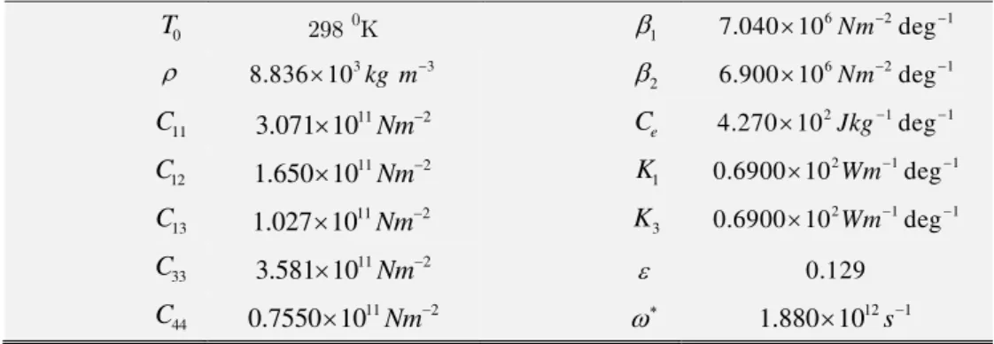
The numerical computation is carried out over a cobalt plate. Physical data for this material are given as:

0

T 298 0K 1

6 2 1

7.040 10 Nm deg

 3 3

8.836 10 kg m ₂ 6 2 1

6.900 10 Nm deg

11

C 11 2

3.071 10 Nm Ce

2 1 1

4.270 10 Jkg deg

12

C 11 2

1.650 10 Nm K1

2 1 1

0.6900 10 Wm deg

13

C 11 2

1.027 10 Nm K3

2 1 1

0.6900 10 Wm deg

33

C 11 2

3.581 10 Nm  0.129

44

C 11 2

0.7550 10 Nm  1.880 10 12s1

Table 1: Physical data for a single crystal of cobalt.

Figures 1-3 depict the slowness surfaces for the thermoelastic single crystal of cobalt whose physi-cal data is given in Table-1. Each figure exhibit the four surfaces one for quasi-longitudinal, two for quasi-shear and one for quasi-thermal. Figure 1-3 represent the slowness surfaces for when

thermal relaxation time increases from 13

1 10  secs to1 10 11secs. From the figures it is observed

that on increasing the thermal relaxation time slowness surfaces for quasi-shear modes have no effect on varying the thermal relaxation time, whereas quasi-longitudinal and quasi-thermal modes are highly affected by the thermal relaxation variations. The inner two curves correspond to the quasi-longitudinal and quasi-thermal wave modes whereas the outer two curves correspond to the two quasi-shear wave modes. Shapes of all the four slowness curves are circular or ellipti-cal.

The innermost curve corresponds to the quasi-thermal (qT) wave mode, next from the inner is

the quasi-longitudinal(qL) mode the one with dimples to the quasi-shear (qSV) wave, and the

outer elliptical surface to the quasi-shear (qSH) wave. In slowness space, the four slowness

surfac-es for the qT, ql, qSV, and qSH waves are from innermost to outermost are obtained.

Figure 1: Thermoelastic slowness surfaces for crystal of cobalt when thermal relaxation time is 13

1 10  secs.

3.5104 2.1104 7105 7105 2.1104 3.5104

4104 2.4104 8105 8105 2.4104 4104

Slowness x1

Sl

ow

nes

s x

(8)

Figure 2: Thermoelastic Slowness surfaces for crystal of cobalt when thermal relaxation time is 12

1 10  secs.

Figure 3: Thermoelastic Slowness surfaces for crystal of cobalt when thermal relaxation time is 11

1 10  secs.

Figure 4: Thermoelastic Slowness surfaces for crystal of cobalt when thermal relaxation time is equalto zero.

3.5104 2.1104 7105 7105 2.1104 3.5104

4104 2.4104 8105 8105 2.4104 4104

Slowness x1

Sl

owne

ss x3

8104 4.8104 1.6104 1.6104 4.8104 8104

Slowness x1

Slowness x3

3.5104 2.1104 7105 7105 2.1104 3.5104

4104 2.4104 8105 8105 2.4104 4104

Slowness x1

Slowne

ss

(9)

Results for possessing transverse isotropy, whose x1 axis is normal to the plane of isotropy, can be

easily obtained by noting the additional conditions imposed by symmetry, namely

33 22 13 12 55 66 44 22 23 33 22 13 12 55 66 44 22 23

, , , 2

c c c c c c c c c

        

    

And for cubic symmetry

11 22 33

,

12 13 23

,

44 55 66

c



c



c



c



c



c



c

and



₁₁





₂₂





₃₃

Finally, for the isotropic case

11 22 33 2 , 12 13 23

c c c    c c  c 

44 55 66 , j , j , ( 1, 2, 3.)

c c c    K K j

For thermoelastic isotropic solids, the wave-velocity surfaces are concentric spheres in the same way as in corresponding elastic media, where transverse (t) and quasi-transverse (qt) surfaces coincide and all waves are pure mode. In generalized thermoelasticity all waves are not in pure mode, longitudinal and a thermal wave-velocity surface are coupled, and exists as quasi-

longitu-dinal (ql) and quasi-thermal (qth) mode. Shear wave mode decoupled and is not affected by the

thermal fields. Figures 5-8 exhibit polar diagrams of phase velocity (m/s) for an isotropic alumi-num material with different thermal relaxation times. Whereas Figure 9 shows polar diagrams of phase velocity (m/s) for an isotropic aluminum material when coupling constant is zero

In Figure 5, wave-velocity surface corresponding to quasi-longitudinal mode (

ql

) is a sphere with

greater radius than quasi-thermal (qth)mode wave-velocity surface are drawn, when thermal

re-laxation time 13

0 1.363 10



_ _  _{,, and they are in the order}

ql t qth, this shows that

longitudi-nal wave velocity will exceed thermal wave velocity, and the wave velocity of transverse wave

velocity lies between longitudinal and thermal wave velocities. When 13

0 1.379 10

 _ _  _,

( )

ql t qth ,

longitudinal wave velocity exceed thermal wave velocity, and transverse wave velocity become equal to thermal wave velocities is shown in Figure 6.

Figure 5: Polar diagram of phase velocity (m/s) for an isotropic aluminum

material when coupling constant 13

0 1.363 10 s

 _ _  _.

8105 6105 4105 2105 0 2105 4105 6105 8105

8105 6105 4105 2105 2105 4105 6105 8105

(10)

0 1.379 10

 _ _  _.

material when coupling constant 1 4

0 1 .0 1 0 s

 _ _  _.

When 14

0 2.293 10



_ _  _,

( )

qlqth t , and at



₀2.21 10 14, quasi-longitudinal and quasi-thermal

mode conversion take place is shown in Figure 7.

1106 8105 6105 4105 2105 0 2105 4105 6105 8105 1106

1106 5105 5105 1106

Quasi-longitudinal Quasi-thermal Quasi-transverse Transvetrse

8105 6105 4105 2105 0 2105 4105 6105 8105

8105 6105 4105 2105 2105 4105 6105 8105

(11)

0 2.293 10 s

 _ _  _.

……. Wave Surface (ql) *** Wave Surface (qth)

─ Wave surface (transverse t)

material when coupling constant is zero.

8105 6105 4105 2105 0 2105 4105 6105 8105

8105 6105 4105 2105 2105 4105 6105 8105

Quasi-longitudinal Quasi-thermal Quasi-transverse Transvetrse

8105 6105 4105 2105 0 2105 4105 6105 8105

(12)

From the above discussion it is observed that thermo-mechanical stability requires that

vq

_thermal,

5 5

thermal

2.938.10 ( / )m s vq  7.208.10 ( / )m s, while thermal relaxation time 14 13 0

2.293 10 sec  s  1.379 10 sec  s, Thus

,

l th

q q and

t

surfaces cannot cross in the thermo isotropic–solid case, for mechanical stability

requires that

v

l exceed vt 4 / 3. Thus l and

t

surfaces cannot cross in the isotropic–solid case.

Quasi-longitudinal and quasi-thermal surfaces mean that a transverse wave velocity will exceed a longitudinal wave velocity. A longitudinal- transverse mode conversion means that both longitu-dinal and transverse modes exit on the wave surfaces.

6 CONCLUSIONS

In this article analysis for general closed form solution of the thermoelastic waves in anisotropic heat conducting materials is obtained and the solution technique for the secular equation in the framework of the generalized theory of thermoelasticity is employed. Obtained results are general in nature and can be applied to the materials of higher symmetry classes such as transversely isotropic, cubic, and isotropic materials. Uncoupled and coupled thermoelasticity are the particu-lar cases of the obtained results. Numerical computations are carried out for a crystal of cobalt modeled as a transversely isotropic media. The two dimensional slowness curves corresponding to different thermal relaxations are presented graphically and characteristics displayed are analyzed with thermal relaxations. Slowness surfaces for the thermoelastic single crystal of cobalt are ob-tained at different values of thermal relaxation time. Each figure exhibit the four surfaces one for quasi-longitudinal, two for quasi-shear and one for quasi-thermal. It is also observed that on in-creasing the thermal relaxation time, there is no effect of thermal relaxation time on slowness surfaces for quasi-shear modes, whereas quasi-longitudinal and quasi-thermal modes are highly affected by the thermal relaxation variations. Further inner two curves correspond to the quasi-longitudinal and quasi-thermal wave modes whereas the outer two curves correspond to the two quasi-shear wave modes and the shapes of all the four slowness curves are circular or elliptical.

For thermo elastic isotropic solids, the wave-velocity surfaces are concentric spheres in the same way as in its counterpart elastic media, where transverse (t) and quasi-transverse (qt) surfa-ces coincide and all waves are pure mode. In generalized thermoelasticity all waves are not in pure mode, longitudinal and a thermal wave-velocity surface are coupled, and exists as

quasi-longitudinal (ql) and quasi-thermal (qth) mode. Shear wave mode decoupled and is not affected

by the thermal fields. It is observed that thermo-mechanical stability in the case isotropic

mate-rial requires that quasi-longitudinal velocity mode should exceed 4 / 3 times the quasi-transverse

velocity. It is observed that for thermo-mechanical stability in case of quasi-thermal requires,

5 5

2.938.10 ( / ) quasi-thermal 7.208.10 ( / )m s  m s , and thermal relaxation time should be in the range

14 13

0

2.293 10 sec  s  1.379 10 sec  s. Further studies using the above equations and results can be made

(13)

References

Achenbach, J. D.(1975). Wave Propagation in Elastic Solids, North-Holland, Amsterdam. Auld, B. A. (1973). Acoustic waves and fields in solids, vol. 1, New York, NY: Wiley.

Banerjee D. K. and Pao Y. K., (1974). Thermoelastic waves in anisotropy solids”, J. Acoust. Soc. Am. 56:1444-1454.

Bernard C., and Yves, B. (1992). Photoacoustic interactions by modulation and laser impact: Applications in mechanics and physics of anisotropic solids ' J. Acoustique 5: 417-453.

Chandrasekharaiah, D. S. (1986).Thermoelasticity with second sound-A Review, Appl. Mech. Rev., 39: 355-376. Chandrasekharaiah, D. S. 1998. Hyperbolic thermoelasticity.-A review of recent literature. Applied Mechanics Review, 51(12): 705-729.

Chiriţă Stan (2013). On the Rayleigh surface waves on an anisotropic homogeneous thermoelastic half space, Acta Mechanica, 224(3): 657-674.

Dhaliwal, R.S., and Sherief, H. H.(1980) Generalized thermoelasticity of anisotropic media. Quart. Appl. Math. 38: 1-8.

Ewing, W. M., Jardetzky, W. S., and Press, F. (1957). Elastic Waves in Layered Media. McGraw-Hill, New York,.

Graff, K. F. (1975). Wave Motion in Elastic Solids, Oxford University Press, New York, NY, USA. Green, A. E. and Lindsay, K. A. (1972). Thermoelasticity, Journal of Elasticity, 2(1): 1–7.

Kumar, R., Kaur, M. and Rajvanshi S.C., (2014). Propagation of waves in micropolar generalized thermoelastic materials with two temperatures bordered with layers or half-spaces of inviscid liquid, Latin American Journal of Solids and Structures 11:1091-1113.

Lord, H. W. and Shulman Y. A. (1967). Generalized dynamical theory of thermoelasticity, Journal of the Me-chanics and Physics of Solids, 15(5): 299–309.

Love, A. E. H. (1927). Some Problems of Geodynamics. University Press, Cambridge, (reprint: Dover, New York 1967).

Musgrave, M.J.P. (1970). Crystal Acoustics. Holden-Day, San Francisco. (reprint: Acoustical Society of America, New York .

Nayfeh, A. H. (1995). Wave propagation in layered anisotropic media with applications to sites,. North Holland, Amsterdam. Holland, Amsterdam.

Nowacki, W. (1986). Dynamic Problems of Thermoelasticity, P. H. Francis and R. B. Hetnarski, Eds, PWN-Polish Scientific, Warszawa, Poland, 2nd edition,

Sharma, M. D. (2008). Inhomogeneous waves at the boundary of a generalized thermoelastic anisotropic medium, International Journal of Solids and Structures 45: 1483–1496.

Singh Baljeet (2013).Wave propagation in dual-phase-lag anisotropic thermoelasticity, Continuum Mechanics and Thermodynamics , 25( 5): 675-683.

Sura A. and Kanoria, M. (2014). Fractional heat conduction with finite wave speed in a thermo-visco-elastic spherical shell, Latin American Journal of Solids and Structures 11: 1132-1162.

Ting, T. C. T. (1996). Anisotropic Elasticity: Theory and Applications. Oxford University Press, New York. Verma, K. L. (1997). Propagation of generalized thermoelastic free waves in pates of anisotropic media. Proceed-ing of second International Conference on Thermal Stresses and related topics, 199-201.

(14)

Verma, K. L., and Hasebe, N. (2002). Wave propagation in transversely isotropic plates in generalized thermoe-lasticity. Arch. Appl.. Mech. 72(6-7): 470-482.

Verma, K. L., (2002). On The Propagation of Waves In Layered Anisotropic Media in Generalized Thermoelastic-ity, International Journal of Engineering Science, 40(18): 20772096.

Verma, K. L., and Hasebe, N. (2004). On The Flexural and extensional thermoelastic waves in orthotropic with thermal relaxation times,Journal of Applied Mathematics, 1: 69–83.

Verma K. L., (2012). Thermoelastic wave propagation in laminated composites plates, Applied and Computatio-nal Mechanics,6 : 197–208