Dissertation submitted to obtain the degree of Master in Environmental Management Systems Supervisor: Ana Maria Nobre, Postdoctoral Researcher, CIIMAR Co-supervisor: João Gomes Ferreira, Tenured Associate Professor with Agregação, FCT-UNL

(1)

Filipe Miguel Ramos da Cruz Soares

Degree in Environmental Engineering Sciences

Development of tools for the

management of oyster nurseries: static

and dynamic modelling

Dissertation submitted to obtain the degree of Master in Environmental Management Systems

Supervisor: Ana Maria Nobre, Postdoctoral Researcher,

CIIMAR

Co-supervisor: João Gomes Ferreira, Tenured Associate

Professor with Agregação, FCT-UNL

Jury:

President: Prof. Maria Helena Costa Examiner: Prof. Paulo Alexandre Diogo

Examiner: Dra. Ana Maria Nobre

(2)

(3)

Filipe Miguel Ramos da Cruz Soares

Degree in Environmental Engineering Sciences

Development of tools for the

management of oyster nurseries: static

and dynamic modelling

Dissertation submitted to obtain the degree of Master in Environmental Management Systems

Supervisor: Ana Maria Nobre, Postdoctoral Researcher,

CIIMAR

Co-supervisor: João Gomes Ferreira, Tenured Associate

Professor with Agregação, FCT-UNL

Jury:

President: Prof. Maria Helena Costa Examiner: Prof. Paulo Alexandre Diogo

Examiner: Dra. Ana Maria Nobre

(4)

(5)

iii Development of tools for the management of oyster nurseries: static and dynamic modelling

(6)

(7)

v

Acknowledgments

First of all, I would like to thank my supervisor, Ana Nobre, for the opportunity, guidance, support, and for all the trust placed in me. It was a pleasure to work with her, in which I learned a lot. I'm really grateful.

In second, I would like to thank my co-supervisor and professor, João G. Ferreira, the availability and helpful comments during this work. I cannot fail to mention all the guidance, and awareness for certain themes, provided during my years of study. It was very inspiring to me.

I would like to thank Rui Moreira and François Hubert, from Bivalvia, for the opportunity to develop the case study for Bivalvia’s nursery, as well as their availability to provide me all the necessary knowledge and data about the system.

To Richard Langton, for the kindness to provide me some additional information about the experimental conditions of one of his published experiments.

To Joana, for the helpful review of the grammatical construction of writing.

To Julia, for all the patience, support, discussions, and funny moments, which help me a lot during this work.

(8)

(9)

vii

Abstract

Ecological models have been applied for carrying capacity assessments of oyster aquaculture, and have shown to be very useful in guiding the planning and management towards production optimization. However, the existing models are mostly directed to the grow-out phase (production of adult oyster), lacking models to be applied in nurseries (production of juvenile oyster).

This work presents two models to support the management of oyster nurseries that are targeted to farmers:

- A static mass balance model for oyster nurseries, which estimates the maximum stock for typical external food concentrations of the nursery. Part of the work developed herein contributed to its development (available online at:

http://seaplusplus4.com/oysterspatbud.html).

- A dynamic model for oyster nurseries, which simulates the individual growth, food availability and stock evolution over time. The model was conceptualized and implemented as part of this work, and further validated with three data sets from the scientific literature.

In this work, it is shown the application of both models to simulate a commercial nursery. The results show that both models can provide useful information, and thus guidance to farmers, even when there is a lack of data or knowledge about some features of the system, required to properly drive the models.

(10)

(11)

ix

Resumo

Modelos ecológicos têm sido aplicados para a avaliação da capacidade de carga da aquacultura de ostra, demonstrando serem muito úteis na orientação do planeamento e gestão em direção à otimização da produção. No entanto, os modelos existentes são na sua maioria direcionados à fase de engorda (produção de ostra adulta), faltando modelos para serem aplicados em berçários (produção de ostra juvenil).

Este trabalho apresenta dois modelos para apoiar a gestão de viveiros de ostra, e direcionam-se aos produtores:

- Um modelo estático de balanço de massas para viveiros de ostra, o qual para típicas concentrações de alimento no exterior do berçário estima o máximo estoque a sustentar. Parte do trabalho desenvolvido aqui contribuiu para o seu desenvolvimento (disponível online em: http://seaplusplus4.com/oysterspatbud.html).

- Um modelo dinâmico para viveiros de ostra, que simula o crescimento individual, a disponibilidade de alimento e a evolução do estoque ao longo do tempo. O modelo foi conceptualizado e implementado como parte deste trabalho, e validado para três conjuntos de dados da literatura científica.

Neste trabalho, mostra-se a aplicação de ambos os modelos para simular um viveiro comercial. Os resultados mostram que ambos os modelos podem fornecer informações úteis e, portanto, orientações aos produtores, mesmo quando há falta de dados ou conhecimento sobre algumas características do sistema, necessários para correr adequadamente os modelos.

(12)

(13)

xi

List of Figures

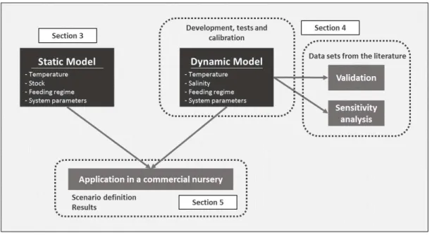
Figure 2.1 - Thesis Framework. ... 5

Figure 2.2 - Commercial nursery location: A) Portugal; B) Ria Formosa; C) and D) – Satellite view of the commercial nursery. ... 6

Figure 2.3 - Scheme of the commercial nursery FLUPSY (top view), where the arrows represent the direction of the water flow and: A) Oyster silos with mesh bottom; B) Central water

channel; C) Rearing tank; D) Intermediate tank; E) Propeller; F) Floaters. ... 7

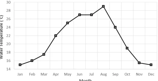
Figure 2.4 - Mean monthly water temperature in the commercial nursery. ... 8

Figure 3.1 - Conceptual model for the oyster nursery. ... 14

Figure 3.2 - Overall organization of model interface. Four menus: Nursery parameters, Output for food requirements, Output for optimum stock, Biological advanced settings. Full online interface available at http://seaplusplus4.com/oysterspatbud.html. ... 21

Figure 3.3 - Model interface: nursery parameters. Full online interface available at

http://seaplusplus4.com/oysterspatbud.html... 22

Figure 3.4 - Model interface: model outputs for minimum external food concentration for a given stock. Full online interface available at http://seaplusplus4.com/oysterspatbud.html. .. 23

Figure 3.5 - Model interface: model outputs for maximum stock that can be sustained for a given food input and considering a given stock distribution per grades. Full online interface available at http://seaplusplus4.com/oysterspatbud.html. ... 24

Figure 3.6 - Model interface: advanced biological parameters (user defined). Full online

interface available at http://seaplusplus4.com/oysterspatbud.html. ... 25

Figure 3.7 - Model application for quantification of general rules of thumb about biomass stock that can be sustained by blooming ponds: a) model setup, b) model outputs considering spat of about 0.38g, b) model outputs considering spat of about 0.04 g. ... 28

Figure 4.1 - Scheme of the oyster spat individual bioenergetic model (based on Kobayashi et al., 1997; Bayne, 1999; Gosling, 2004). ... 32

Figure 4.2 - Conceptual food mass balance model for an oyster spat production unit, where M_index represents mass and _MFindex represents mass flows (based on Chapra, 1997). ... 39 Figure 4.4 - Simulated and observed growth of Crassostrea gigas spat, for Exp A from Langton and McKay (1976) dataset (Table 4.3). ... 44

(16)

xiv

Figure 4.6 - Simulated and observed growth of Crassostrea gigas spat, for Exp Favorable from Claus et al., (1983) dataset (Table 4.3). ... 45

Figure 5.1 - Relative increase in maximum simulated stock due to water temperature effects, in

relation to a standard stock simulated at 19˚C. ... 54

Figure 5.2 – Simulations of Crassostrea gigas spat individual growth and tank concentration for Scenario 1. The individuals are classified by batch according to the initial weight (T4, T6, T8). 58

(17)

xv

List of Tables

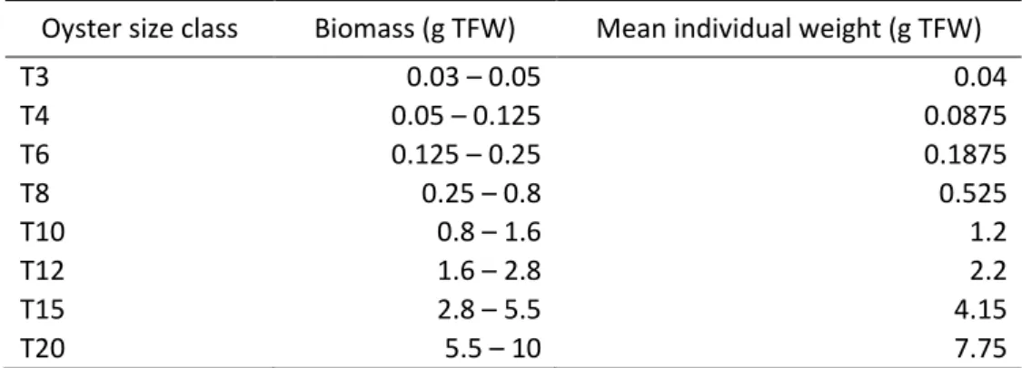
Table 2.1 - Biomass and mean individual weight of the commercial nursery oyster size class. ... 7

Table 3.1 - Oyster food indicators and corresponding model units... 14

Table 3.2 - List of model parameters. ... 16

Table 3.3 - Model parameterization for Pacific oyster (Crassostrea gigas Thunberg). ... 19

Table 3.4 - Model settings to simulate Langton & McKay (1976) experiments. ... 20

Table 3.5 - Examples of nursery system definition for different types of nurseries (FLUPSY, Land-based with blooming tanks and closed systems). ... 22

Table 3.6 - Model outputs for Langton & McKay (1976) experiments. ... 26

Table 4.1 – Variables, parameters, conversion factors and functions of the model. ... 32

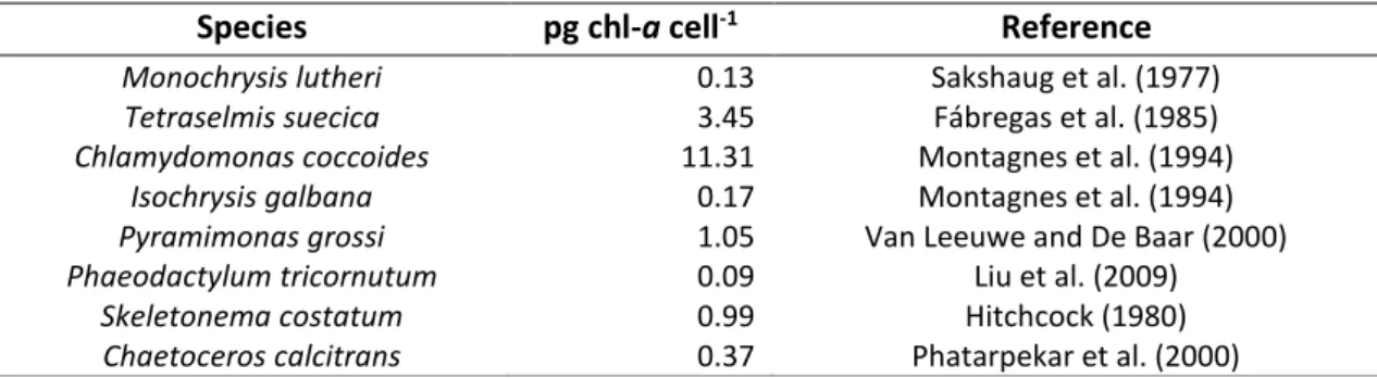
Table 4.2 –Chl-a content, by phytoplankton species, expressed as pg chl-a cell-1_{. ... 34}

Table 4.3 – Settings of the dynamic model for oyster nurseries to simulate Langton and McKay (1976) and Claus et al. (1983) experimental conditions. ... 43

Table 4.4 –Statistical tests, Pearson’s correlation coefficient (r) and index of agreement (d2). 46 Table 4.5 – Sensitivity analysis of the dynamic oyster model, for changes in plus and minus 10% on model parameters, applied for Exp Favorable from Claus et al., (1983) dataset. ... 46

Table 5.1 – Stocking scenarios and distribution per oyster size class, for the application of the static mass balance model for oyster nurseries. ... 49

Table 5.2 – Model settings for the application of the static mass balance model for oyster nurseries, for different scenarios. ... 50

Table 5.3 – Maximum stock, expressed by weight (kg) and number of individuals (x106 individuals), for each scenario concerning different stock distributions. ... 52

Table 5.4 – Model settings for the application of the dynamic oyster model on different scenarios... 55

(18)

(19)

xvii

List of Abbreviations

ADCP – Acoustic Doppler Current Profiler Chl-a– Chlorophyll-a

DEB – Dynamic Energy Budget DW – Tissue Dry Weight

FAO – Food and Agricultural Organization of the United Nations FLUPSY – Floating Upwelling System

IMTA – Integrated Multi-Trophic Aquaculture NEB – Net Energy Balance

NOAA – National Oceanic and Atmospheric Administration NS – North System

POC – Particulate Organic Carbon POM – Particulate Organic Matter SFG – Scope For Growth

SMR – Standard Metabolic Rate SS – South System

(20)

(21)

1

1. Introduction

Aquaculture was responsible for 53% of the global seafood production (in quantity) in 2015 (FAO, 2017a). At global level stands as the fastest growing food sector, with production increasing at an average of about 6% per annum since the start of the millennium (FAO, 2017a). Prospects point that in the future aquaculture will play an increasingly important role in the

supply of seafood (Msangi et al., 2013; Kobayashi et al., 2015). On the one hand world’s human

population is increasing fast (FAO, 2017b; Samir & Lutz, 2017), which means a higher demand for food in the future, on the other hand the marine biodiversity is being threatened by overfishing, pollution and habitat destruction (Lotze et al., 2006; Halpern et al., 2007; Zhou et al., 2015), which can lead to a crisis in global fisheries by mid-century (Worm et al., 2006; Pauly & Zeller, 2017). Bringing new solutions to the aquaculture sector, aiming a sustainable improvement of its production potential, is a key-point to maintain the growth of the sector. One important share of this sector is the bivalve production. Latest data from FAO (2017), relative to 2015, point that bivalve production accounts for 14% of global aquaculture production (in quantity), of which oysters represent 36%. Aquaculture stands as the main source of oyster production (~97%), being the Asian continent the larger contributor with around 95% of the global farmed volume, followed by the American and European continents (around 3% and 2%, respectively). The Pacific Oyster (Crassostrea gigas, Thunberg) stands out as the most significant species from all the world’s oyster production (FAO, 2017a). It presents a considerable economic value and it is seen as an attractive species by farmers due to its rapid growth in comparison with other oyster species (Ruesink et al., 2005).

Oyster production in aquaculture typically involves three stages: (i) hatchery, specialized in the development of early stages of these organisms (i.e. larvae and small spat), occurring these operations generally in land-based farms; (ii) nursery, focused on rearing oyster spat (seeds) until reaching a sufficient size to be planted in the field, with operations occurring in closed or open upwelling systems (e.g. FLUPSY); and (iii) grow-out, the oyster farming in the field (e.g. estuaries) until they reach the harvestable size to be commercialized, whereby several farming methods can be used, including on-bottom and off-bottom cultures (Flimlin, 2000; Helm & Bourne, 2004; Doiron, 2008).

(22)

2 production cycle rely on the availability of food in the surrounding environment, with exceptions for hatchery operations where the early stages of this organisms are fed with cultured microalgae (Helm & Bourne, 2004). As oysters do not need external feed inputs, like other non-fed cultures (e.g. seaweeds, carps, and other filter-feeding shellfish), their production is seen as attractive. Furthermore, oyster farming can be included in an integrated multi-trophic aquaculture (IMTA), in which organic waste from other adjacent fed aquacultures (e.g. of finfish) can contribute as an additional source of food, thus enhancing the oyster growth or the production capacity, while the oysters, on the other hand, can act as reducers of the environmental impact of organic waste from fish-farming activities (see e.g. Ferreira et al., 2012; Jiang et al., 2013). Other potential ecosystem and ecological benefits, provided by oyster farming, are nowadays widely recognized, including nutrient cycling, top-down control of primary symptoms of eutrophication, benthic-pelagic coupling, refuge from predators, and among others (Dumbauld et al., 2009; Forrest et al., 2009; Higgins et al., 2011). Of relevant importance for farmers are the processes of nutrient cycling and the benthic-pelagic coupling, which may in some cases be translated into an opportunity for additional profit, either by the potential of farmers to benefit, in the near future, from nutrient credit trading programs (Jones et al., 2010; Newell & Mann, 2012; Filgueira et al., 2015a; Ferreira & Bricker, 2016), or by the potential of inclusion of other cultures, in an IMTA, to reuse the deposited organic waste of oyster farms (see e.g. Paltzat et al., 2008).

(23)

3 Ecological models have proven to be useful in this assessment (see e.g. Duarte et al., 2003; Nunes et al., 2003; Grant et al., 2007; Ferreira et al., 2007; Guyondet et al., 2010), thus becoming powerful tools to be used by shellfish farmers or consultants related with this sector. Models developed in this scope usually incorporate a different set of sub-models, as: (i) a hydrodynamic model, which simulates the motion, transportation and transfer of particles or substances (e.g. food and nutrients); (ii) a primary production model, that simulates the primary production within the considered system; and (iii) a bioenergetic model, which simulates the energy allocation in a certain bivalve species under different food and environmental conditions. Some of this models include other components (e.g. ecological and economic), and couple the bioenergetics modelling of more than one species (Nunes et al., 2003; Ferreira et al., 2007). Bioenergetic models of bivalves are constructed based on mathematical functions that represent the physiological processes of an organism, which requires a broader knowledge of its physiology. In the majority of the cases, this functions derive from laboratory experimental data, depending its formulation on the conditions of the experiments, e.g. temperature, salinity, suspended matter quality and quantity, among others (e.g. Bayne, 1999; Ren et al., 2000). The conceptualization of this models is based on theories of energy allocation. Traditional bioenergetics theories, e.g. net energy balance (NEB) or scope for growth (SFG), describe energy acquisition from feeding and its partitioning among processes as respiration, activity, reproduction, excretion and growth (Winberg, 1960), whilst the energy budget (DEB) theory (Kooijman, 2000) describes the individual in terms of structural body and reserves, being that the energy acquired from feeding is allocated to the reserves before being used for somatic maintenance, growth, maturity maintenance, maturation and reproduction (van der Meer, 2006).

(24)

4 Given that oyster nurseries are commonly extensive systems, as they hinge on the food available in the surrounding environment, and in some cases from phytoplankton blooming ponds (used to induce phytoplankton growth), ecological models may play an important role in the nursery management and sustainability assessments (e.g. models to assess the production carrying capacity). However, models of this type, applicable in oyster nurseries, are lacking from the scientific literature.

1.1. Objectives

The work developed herein intends to fill the lack of ecological models applicable to oyster nurseries, aiming:

- A simplified simulation of the oyster nursery to assess the maximum stock sustained, by means of a static model.

- A dynamic simulation of oyster spat individual growth, food availability within the farming system and stock biomass, by means of a dynamic model.

It is expected that these models can be used as tools for the management of oyster nurseries, by providing knowledge about the system behavior under different conditions.

(25)

5

2. General approach

2.1. Overview

Taking into account that the level of knowledge about the system conditions may differ among oyster nurseries managers, it was followed two modelling approaches: (i) a static and simplified, which requires a lower level of input data, but which in turn provides limited output data; and (ii) a dynamic, which requires a higher level of input data, thus providing a wider range of output data. Despite the differences, both approaches have the common objective of guiding the management for production optimization.

For an overall assessment of the maximum stock for typical external food concentrations at the nursery a static mass balance model for oyster nurseries was used (Section 3, available online

at: http://seaplusplus4.com/oysterspatbud.html). This model resulted from a collaborative

work, in which part of it was developed within the scope of this thesis. The final work was consolidated into a research paper (presented in Section 3), which was accepted for publication by the Journal of Shellfish Research.

Figure 2.1 - Thesis Framework.

(26)

6 Both models were applied in a commercial nursery, operated by Bivalvia – Mariscos da Formosa, Lda (Section 5). Hypothetical scenarios were defined and guided by the farm operational manager and aimed at the identification of key-factors for production optimization.

2.2. Case study

–

Bivalvia

’s

commercial nursery

Bivalvia’s nursery is located within the Ria Formosa (37°00'58.6"N and 7°52'55.8"W, Figure 2.2), a complex inshore coastal system located in southern Portugal, with the status of marine protected area. With an extent of 55 km (W-E) and 6 km (N-S), the Ria Formosa is separated from the sea by sandbanks and several barrier islands. The tidal range is between 0.9 and 3.0 m (Ferreira et al., 2014), being considered as mesotidal. About 50 to 75% of its water volume is renewed daily due to the tides (Newton & Mudge, 2003), becoming the large mudflats exposed at low tide and submerged at high tide (Neves, 1988).

Figure 2.2 - Commercial nursery location: A) Portugal; B) Ria Formosa; C) and D) – Satellite view of the commercial nursery.

At the national level the Ria Formosa stands as the most productive aquaculture zone, being simultaneously the home of multiple socio-economic activities such as tourism, salt extraction, fisheries, effluent discharges, among others (Ceia et al., 2010; Ferreira et al., 2013; Ferreira et al., 2014).

(27)

7 The FLUPSY (Figure 2.3) is a shellfish nursery system designed to increase the water flow efficiency, and therefore the rate at which the food is delivered to the post-settled shellfish. Usually, this type of systems are placed in productive coastal waters and are incorporated into a floating dock (Meseck et al., 2012).

Figure 2.3 - Scheme of the commercial nursery FLUPSY (top view), where the arrows represent the direction of the water flow and: A) Oyster silos with mesh bottom; B) Central water channel; C) Rearing tank; D) Intermediate tank; E) Propeller; F) Floaters.

In the commercial nursery, the oyster spat are placed inside silos with mesh bottoms (A), divided by size classes (Table 2.1), where an upwelling current flows through it. The silos are connected to a central water channel (B), which in turn is connected to an intermediate tank (D). An electric propeller (E), installed on the boundary that separates the intermediate tank from the phytoplankton blooming ponds, induce the current by expelling the water to the phytoplankton blooming ponds.

Table 2.1 - Biomass and mean individual weight of the commercial nursery oyster size class. Oyster size class Biomass (g TFW) Mean individual weight (g TFW)

T3 0.03 – 0.05 0.04

T4 0.05 – 0.125 0.0875

T6 0.125 – 0.25 0.1875

T8 0.25 – 0.8 0.525

T10 0.8 – 1.6 1.2

T12 1.6 – 2.8 2.2

T15 2.8 – 5.5 4.15

(28)

8 The commercial nursery operates with just one phytoplankton blooming pond connected to the FLUPSY, while the other remains without use to accumulate phytoplankton biomass. The daily water renewal is about 2 to 5% of the production tank volume. Each phytoplankton blooming pond has an approximate area of 70 000 and 54 000 m2_{(NS and SS respectively) with an average}

depth of 1 m. The rearing tank has an area of about 1 000 m2_{with an average depth of 1.3 m.}

Considering a total water mix in each blooming pond, i.e. without “dead zones”, it is assumed a overall system volume of 71 300 m3_{when NS is operating, and a volume of 55 300 m}3_{for the}

case of SS being in operation.

Along the year water salinity remains at 36 psu, with minor fluctuations, and the water temperature ranges between 15 and 29˚C (Figure 2.4, François Hubert, Bivalvia, personal communication). Historic water samples indicate a phytoplankton concentration inside the production tank up to about 200 cells µL-1_{, and a phytoplankton concentration in the external}

water channel ranging between 0.3 – 1.0 cells µL-1_{(François Hubert, Bivalvia, personal}

communication). These water samples were only carried out for some months, for short intervals, and done with the production system working, not allowing a good representation of the system conditions during all the year as well as an accurate initial tank concentration.

(29)

9

3. A static mass balance model for oyster nurseries

This section presents a static mass balance model, which can be used to assess the feeding requirements of a given stock or the maximum stocks sustained for a given feeding regime within an oyster nursery.

(30)

10 This section corresponds to a manuscript currently accepted for publication to the Journal of Shellfish Research:

(31)

11

A mass balance model to assess food limitation in commercial oyster nurseries

ABSTRACT

This work presents a modelling application designed to provide practical guidance about food limitation in oyster nurseries for seed stock management. The model was implemented and evaluated for the Pacific oyster (Crassostrea gigas Thunberg). Scientific knowledge about feeding activity of oyster spat was embedded into a single compartment mass balance. This approach applies to enclosed nurseries such as floating upwelling systems (FLUPSY) or land-based tanks. The mass balance model estimates the i) optimal stock as a function of typical external food concentrations, or ii) the food concentration required for a given stock.

Overall this work aims to support oyster farming which is an important activity from a socio-economic standpoint and for the provision of ecosystem services. While existing ecological models are widely applied for understanding the interactions between the wider ecosystem and farming systems, models are seldom targeted and used directly by farmers. Oyster farmers can use the model to improve the application of general rules of thumb to estimate the stock biomass to hold in their nursery. The mass balance model presented herein is available online (http://seaplusplus4.com/oysterspatbud.html) for widespread use.

INTRODUCTION

(32)

12 by some governmental stakeholders as providing social and economic benefits besides the ecological benefits, e.g. NOAA established in 2011 the USA National Shellfish Initiative.

Most oyster farming practices depend on the natural environment, and like many other farmed species their growth and production hinge on a complex interaction of factors such as temperature, salinity, upstream freshwater flow/rainfall, current speed, density, food concentration and type of the phytoplankton community, food partitioning with other species and disease outbreaks. Modelling can be useful for understanding the feedback between the farming and environmental systems and the effects on production. As an example, carrying capacity models are often applied for management and spatial planning of filter feeder production, as reviewed by Byron & Costa-Pierce (2013) and by Filgueira et al. (2015b). Many other model applications exist for integrated management of oysters and other shellfish production including at ecosystem and farm scales (e.g., Cerco & Noel 2007, Ferreira et al. 2011, Filgueira et al. 2015b, Gangnery et al. 2011, Nobre et al. 2011). Farmers are seldom the target end-users of these models. A strategy to make available simulation models that embed scientific research to farmers is to shift from i) complex models (in terms of spatial and temporal resolutions, processes simulated) that allow detailed simulations but require dataset s that might not be feasible to gather by a commercial unit, to ii) simple models or at least with simple interfaces that can be directly used by farmers and provide estimates of key questions for production; e.g. http://www.farmscale.org/ and Nobre et al. (2017).

(33)

13 al. 1995, Cranford et al. 2011, Gerdes 1983a, Tamayo et al. 2014, Walne 1972, Ward & Shumway 2004, Winter 1978).

Mass balance models can help to translate scientific knowledge into practical guidance for commercial nurseries using simple user interfaces. The goal of this paper is to develop and evaluate this concept using the Pacific oyster (Crassostrea gigas Thunberg) spat as a case study for model implementation and evaluation for enclosed systems such as a floating upwelling system (FLUPSY) or land-based tanks, silos, or trays. The objective is to make the model available online for wider usability and it should tackle two questions that arise when planning or managing an oyster nursery: How much food is required to sustain a given stock and/or for a typical range of food available at surrounding environment what is the maximum biomass to stock in the farm. Further work can be developed for model implementation for other relevant species depending on available research literature and farmers interest: eastern oyster (Crassostrea virginica Gmelin), European flat oyster (Ostrea edulis Linnaeus), Olympia oyster (Ostrea lurida Carpenter), Portuguese oyster (Crassostrea angulata Lamarck), slipper cupped oyster (Crassostrea iredalei Faustino), Sydney rock oyster (Saccostrea glomerate Gould).

METHODOLOGY

Conceptual model description

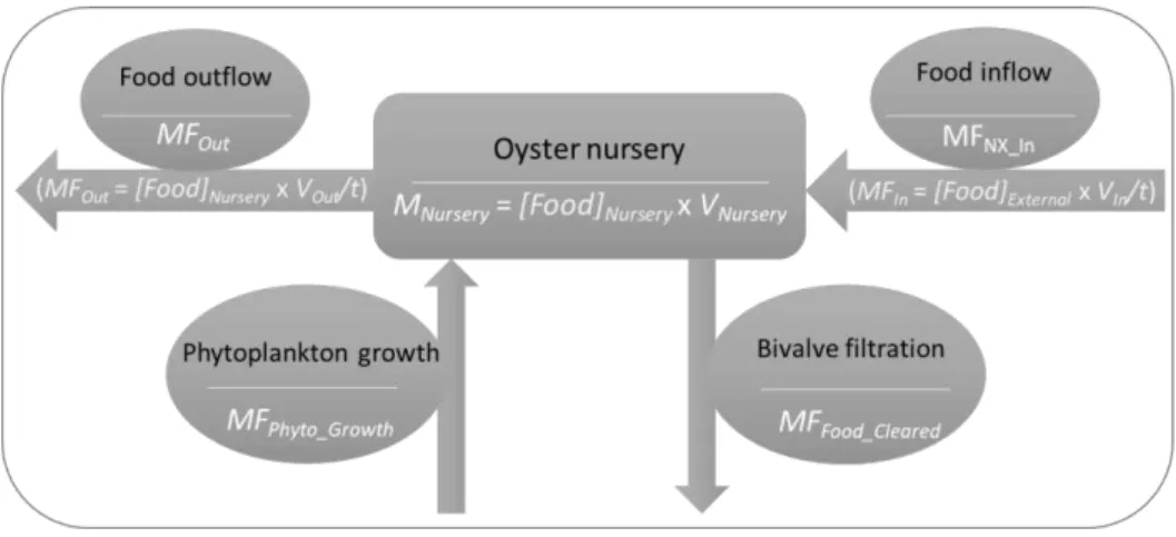
The model developed herein estimates two independent outputs: i) the required food inputs for a given stock biomass and ii) the maximum stock biomass given a typical external food concentration. It consists of a one compartment mass-balance at steady-state (Figure 3.1):

𝑀𝐹𝐹𝑜𝑜𝑑_𝑖𝑛 + 𝑀𝐹𝑃ℎ𝑦𝑡𝑜_𝐺𝑟𝑜𝑤𝑡ℎ= 𝑀𝐹𝐹𝑜𝑜𝑑_𝑜𝑢𝑡+ 𝑀𝐹𝐹𝑜𝑜𝑑_𝐶𝑙𝑒𝑎𝑟𝑒𝑑 (Eq. 3.1)

Whereby, i) the compartment represents an oyster nursery, ii) sources include food inflow (MFFood_in, Eq. 3.2) and phytoplankton growth (MFPhyto_Growth, Eq. 3.3), and iii) sinks include food

cleared by oysters (MFFood_Cleared, Eq. 3.5) and food outflow (MFFood_out, Eq. 3.4). The model is

targeted at extensive farmers that rely on external natural food resources, represented by

MFFood_in. It can also be applied to fed systems considering in that term (i.e., MFFood_in) the feed

ration. The model also includes phytoplankton growth (MFPhyto_Growth) to accommodate the cases

of nurseries with food supplied by phytoplankton blooming ponds (if that is not the case then

(34)

14

Figure 3.1 - Conceptual model for the oyster nursery.

Oyster food can be expressed using different indicators, such as phytoplankton (or its proxy

chl-a), particulate organic matter (POM) and particulate organic carbon (POC), among other. To allow model generality food parameters are expressed using several optional oyster food indicators (Table 3.1).

Table 3.1 - Oyster food indicators and corresponding model units.

Oyster food indicator

Corresponding model units Food concentration:

[Food]External and [Food]nursery

Food fluxes: MFx

Phytoplankton (or a proxy

chl-a) Algae biovolume Per w at e r v o lu m e

mm3_algae.L-1

Per ti

me

mm3_algae.day-1

Cell count algal cells.µL-1 ₁₀6_{algal cells.day}-1

Algal mass mg algae.L-1 _{mg algae.day}-1

Chl-a mass µg Chl-a.L-1 _{µg Chl-}_a_.day-1

POM Mass mg POM.L-1 _{mg POM.day}-1

POC Mass mg POC.L-1 _{mg POC.day}-1

All mass fluxes (MFX, Figure 3.1) are expressed in one of the food indicators (defined in Table

3.1) per time and are defined as follows:

MFFood_in, (Eq. 3.2) is given by the external food concentration ([Food]External, units defined in Table

3.1) multiplied by water inflow (Vin/t, in m3.d-1):

𝑀𝐹𝐹𝑜𝑜𝑑_𝑖𝑛= [𝐹𝑜𝑜𝑑]𝐸𝑥𝑡𝑒𝑟𝑛𝑎𝑙 . 𝑉𝑖𝑛⁄ . 𝑀3𝑡𝑜𝐿𝑡 (Eq. 3.2)

MFPhyto_Growth (Eq. 3.3) stands for the primary production in the nursery system (if applicable),

which is given by the phytoplankton specific growth rate (Growthphyto, d-1) multiplied by the

phytoplankton mass inside the nursery:

𝑀𝐹𝑃ℎ𝑦𝑡𝑜_𝐺𝑟𝑜𝑤𝑡ℎ= 𝐺𝑟𝑜𝑤𝑡ℎ𝑝ℎ𝑦𝑡𝑜 . [𝐹𝑜𝑜𝑑]𝑛𝑢𝑟𝑠𝑒𝑟𝑦 . 𝑉𝑛𝑢𝑟𝑠𝑒𝑟𝑦 . 𝑓𝑟𝑎𝑐𝑡𝑖𝑜𝑛𝑝ℎ𝑦𝑡𝑜 𝑓𝑜𝑜𝑑⁄ . 𝑀3𝑡𝑜𝐿 (Eq. 1.3)

(35)

15 the food. For the cases where the food indicator is phytoplankton fractionphyto/food is one, for the

cases where the food indicator is POM or POC the average fraction of phytoplankton in the food must be defined.

MFFood_out, (Eq. 3.4) is given by [Food]nursery multiplied by the water outflow (Vout/t, in m3.d-1):

𝑀𝐹𝐹𝑜𝑜𝑑_𝑜𝑢𝑡 = [𝐹𝑜𝑜𝑑]𝑛𝑢𝑟𝑠𝑒𝑟𝑦 . 𝑉𝑜𝑢𝑡⁄ . 𝑀3𝑡𝑜𝐿𝑡 (Eq. 3.4)

MFFood_Cleared (Eq. 3.5) is given by the [Food]nursery multiplied by the water volume cleared by the

standing stock in a given period of time (𝐶𝑙𝑒𝑎𝑟𝑎𝑛𝑐𝑒𝑅𝑎𝑡𝑒𝑜𝑦𝑠𝑡𝑒𝑟 . 𝑆𝑡𝑜𝑐𝑘 . 𝐷𝑊𝑡𝑜𝐹𝑊 . 𝑘𝑔_𝑡𝑜_𝑚𝑔); whereby ClearanceRateOyster (L. mg DW-1 . h-1) is the oyster specific clearance rate, Stock (in Kg) is the spat

total biomass in the tanks, and DWtoFW (-) is the conversion ratio of dry weight:fresh weight with shell:

𝑀𝐹𝐹𝑜𝑜𝑑_𝐶𝑙𝑒𝑎𝑟𝑒𝑑= [𝐹𝑜𝑜𝑑]𝑛𝑢𝑟𝑠𝑒𝑟𝑦 . 𝐶𝑙𝑒𝑎𝑟𝑎𝑛𝑐𝑒𝑅𝑎𝑡𝑒𝑜𝑦𝑠𝑡𝑒𝑟 . 𝑆𝑡𝑜𝑐𝑘 . 𝐷𝑊𝑡𝑜𝐹𝑊 . 𝑘𝑔_𝑡𝑜_𝑚𝑔 (Eq. 3.5) M3toL, kg_to_mg and kg_to_g are conversion factors for unit consistency in Eq. 3.2 to Eq. 3.6. The generic model solution for the questions that this work aims to address is given by Eq. 3.6 and Eq. 3.7. These are obtained by considering Vout/t = Vin/t and replacing Eq. 3.2 to Eq. 3.5 into

Eq. 3.1 and solving the mass balance in order to the external food concentration (Eq. 3.6) and in order to stock biomass (Eq. 3.7):

[𝐹𝑜𝑜𝑑]𝐸𝑥𝑡𝑒𝑟𝑛𝑎𝑙= [𝐹𝑜𝑜𝑑]𝑛𝑢𝑟𝑠𝑒𝑟𝑦. (1 − 𝐺𝑟𝑜𝑤𝑡ℎ𝑝ℎ𝑦𝑡𝑜 .𝑉𝑛𝑢𝑟𝑠𝑒𝑟𝑦_𝑉_𝑖𝑛_⁄_𝑡 . 𝑓𝑟𝑎𝑐𝑡𝑖𝑜𝑛𝑝ℎ𝑦𝑡𝑜 𝑓𝑜𝑜𝑑⁄ + 𝐶𝑙𝑒𝑎𝑟𝑎𝑛𝑐𝑒𝑅𝑎𝑡𝑒𝑜𝑦𝑠𝑡𝑒𝑟

𝑉𝑖𝑛⁄𝑡 . 𝑆𝑡𝑜𝑐𝑘. 𝐷𝑊𝑡𝑜𝐹𝑊. 𝑘𝑔_𝑡𝑜_𝑔) (Eq. 3.6)

Stock =[Food]External.Vin⁄ +[Food]nursery.(Growtht phyto.Vnursery.fractionphyto food⁄ −Vin⁄ )t

[Food]nursery .ClearanceRateoyster .DWtoFW .kg_to_g (Eq. 3.7)

Because of the steady-state assumption, the [Food]nursery is a constant; whereby the sinks and

sources of the mass balance are solved to ensure that concentration in the nursery system. That parameter ([Food]nursery) is used in the model as the optimum concentration to maintain in the

production unit. Depending on the available data it can be parameterized as the minimum food concentration that maximizes ingestion or as the optimum concentration for growth. Winter

(1978) argues that bivalve’s filtration efficiency depends on food concentration, whereby “From

a low threshold concentration (A) onwards, filtration rate increases rapidly and is then kept

constant up to a food concentration (B) at which a maximum amount of food is ingested. As soon

as this maximum ingestion rate is reached, the filtration rate decreases continuously in such a

(36)

16

the food concentration (C) is reached at which the production of pseudofaeces begins. At still

higher food concentrations (higher than C) however, filtration and ingestion rate are drastically

reduced”. Thus, this is a key model parameter which allows to impose a minimum concentration that optimizes growth. All the model parameters are systematized in Table 3.2. Other key aspect for model generalization in a simple mass balance while ensuring relevant outputs is the definition of the ClearanceRateOyster as a function of seed weight and water temperature (Eq.

3.8) which must be parameterized per species (or if data is available for a strain within a line): ClearanceRateoyster = f(WaterTemperature, SeedWeight) (Eq. 3.8) Table 3.2 - List of model parameters.

Parameter type Parameter (Unit) Description

Farm p ar ame te rs General settings

Vnursery (m3)

Water volume of the nursery. The boundaries of the system can be the volume encompassed by e.g. the flupsy area or can

further include adjacent ponds for naturally grown phytoplankton communities.

TurnoverRate (day-1₎ Number of volume renewals per day. Should be consistent with

the system boundary.

WaterTemperature (C) An average value should be provided. Temperature inputs are limited to the range between 4C and 30C.

SeedWeightPerGrade(g)

Food indicator To choose from Table 3.1. Model solved

for

[Food]External

StockPerGrade (kg) Stock biomass per grade.

Model solved for

TotalStock

Stock%PerGrade(-)

Fraction of the stock for a given grade relative to the total biomass.

[Food]External

Typical external food concentration or feed supplementation. The model implementation allows testing of two values. Units

depend on the food indicator chosen (Table 3.1).

Bi ol ogi cal p ar am. (ad v an ce d ) Species- specific [Food]nursery

Optimum food concentration for oyster filtration. Units depend on the food indicator chosen (Table 3.1).

DWtoFW (-) Conversion ratio of dry weight:fresh weight with shell.

ClearanceRateOyster (L. mg DW-1_{. h}-1₎

The clearance rate is a model parameter that in fact is a function of seed weight and water temperature and is

species-specific.

Site specific

Growthphyto(day-1)

Specific local phytoplankton community growth rate. If values are not known a range within two values can be tested.

fractionphyto/food (-)

Average typical values of the fraction of phyto in the food applicable for the cases where food indicator is POM or POC.

When food indicator is algae this parameter is one.

For a practical application of this model the user can define Vin/t as flow rate or by the

operational turnover rate (TurnoverRate , d-1_{) multiplied by the nursery volume (Eq. 3.9):}

(37)

17 To be useful for real farms the model was extended to consider the simultaneous cultivation of several spat grades:

i) Eq. 3.10 to estimate required external food concentration considering the summation of the volume cleared per grade (∑ 𝐶𝑙𝑒𝑎𝑟𝑎𝑛𝑐𝑒𝑅𝑎𝑡𝑒_{𝑂𝑦𝑠𝑡𝑒𝑟_𝑃𝑒𝑟𝐺𝑟𝑎𝑑𝑒}. 𝑆𝑡𝑜𝑐𝑘𝑃𝑒𝑟𝐺𝑟𝑎𝑑𝑒):

[𝐹𝑜𝑜𝑑]𝐸𝑥𝑡𝑒𝑟𝑛𝑎𝑙= [𝐹𝑜𝑜𝑑]𝑛𝑢𝑟𝑠𝑒𝑟𝑦. (1 − 𝐺𝑟𝑜𝑤𝑡ℎ𝑝ℎ𝑦𝑡𝑜 .𝑉𝑛𝑢𝑟𝑠𝑒𝑟𝑦_𝑉_𝑖𝑛_⁄_𝑡 . 𝑓𝑟𝑎𝑐𝑡𝑖𝑜𝑛𝑝ℎ𝑦𝑡𝑜 𝑓𝑜𝑜𝑑⁄ + ∑ 𝐶𝑙𝑒𝑎𝑟𝑎𝑛𝑐𝑒𝑅𝑎𝑡𝑒_{𝑂𝑦𝑠𝑡𝑒𝑟_𝑃𝑒𝑟𝐺𝑟𝑎𝑑𝑒}.𝑆𝑡𝑜𝑐𝑘𝑃𝑒𝑟𝐺𝑟𝑎𝑑𝑒

𝑉𝑖𝑛⁄𝑡 . 𝐷𝑊𝑡𝑜𝐹𝑊. 𝑘𝑔_𝑡𝑜_𝑔) (Eq. 3.10)

ii) Eq. 3.11 to estimate the total maximum stock (TotalStock, in kg) considering a weighted clearance rate (∑ 𝐶𝑙𝑒𝑎𝑟𝑎𝑛𝑐𝑒𝑅𝑎𝑡𝑒_{𝑂𝑦𝑠𝑡𝑒𝑟_𝑃𝑒𝑟𝐺𝑟𝑎𝑑𝑒}. 𝑆𝑡𝑜𝑐𝑘%𝑃𝑒𝑟𝐺𝑟𝑎𝑑𝑒):

𝑇𝑜𝑡𝑎𝑙𝑆𝑡𝑜𝑐𝑘 =[𝐹𝑜𝑜𝑑]𝐸𝑥𝑡𝑒𝑟𝑛𝑎𝑙.𝑉𝑖𝑛⁄ +[𝐹𝑜𝑜𝑑]𝑛𝑢𝑟𝑠𝑒𝑟𝑦.(𝐺𝑟𝑜𝑤𝑡ℎ𝑝ℎ𝑦𝑡𝑜.𝑉𝑡 𝑛𝑢𝑟𝑠𝑒𝑟𝑦.𝑓𝑟𝑎𝑐𝑡𝑖𝑜𝑛𝑝ℎ𝑦𝑡𝑜 𝑓𝑜𝑜𝑑⁄ −𝑉𝑖𝑛⁄ )𝑡

[𝐹𝑜𝑜𝑑]𝑛𝑢𝑟𝑠𝑒𝑟𝑦 .∑ 𝐶𝑙𝑒𝑎𝑟𝑎𝑛𝑐𝑒𝑅𝑎𝑡𝑒𝑂𝑦𝑠𝑡𝑒𝑟_𝑃𝑒𝑟𝐺𝑟𝑎𝑑𝑒.𝑆𝑡𝑜𝑐𝑘%𝑃𝑒𝑟𝐺𝑟𝑎𝑑𝑒 .𝐷𝑊𝑡𝑜𝐹𝑊 .𝑘𝑔_𝑡𝑜_𝑔 (Eq. 3.11)

Also for usability issues and to provide outputs of interest to farmers the final model equations (Eq. 3.10 and Eq. 3.11) are solved for two values of phytoplankton growth (Growthphyto ) and two

values of external food concentration ([Food]External). With this approach, the outputs encompass

the range of scenarios within which a nursery operates, given that these two parameters are highly variable within a day.

As a case study, this model is herein applied to the Pacific oyster. Parameterization for this species is presented in Table 3.3.

Model parameterization and evaluation for the Pacific oyster

[Food]nursery , DWtoFW (-), ClearanceRateOyster, are species-specific and were parameterized

(Table 3.3) for the Pacific oyster based on published data of spat growth experiments.

[Food]nursery was parameterized for the Pacific oyster spat based on Tamayo et al. (2014) which

tested three feed concentrations (0.5, 3, and 6 mm3_.L-1_{); the medium level was chosen given it}

corresponded to the highest clearance rate (for the biological meaning of [Food]nursery see the Conceptual model description section). That concentration level (which converts to 44 algal cells.µL-1_{as per rationale explained herein) is comparable with the range indicated by Walne}

(1972) as the optimum for growth, around 30 to 40 algal cells.µL-1_{. Tamayo et al. (2014) provides}

the conversion of the algal biovolume into POM (Particulate Organic Matter) and POC (Particulate Organic Carbon). Conversion into mg algal.L-1_{considered that the algal cell has the}

(38)

-18

1_{) into algal cell count (algal cells.µL}-1_{) the average cell biovolume for the species used in the}

work by Tamayo et al. (2014), Isochrysis galbana Parke, of around 68 µm3_.cell-1_{(Ishiwata et al.}

2013) was considered. Finally, conversion into Chl-a was carried out using the general conversion ratio of C:Chl-a of around 50 (Reynolds 2006). All values are shown in Table 3.3. Gerdes (1983a) carried out a set of experiments to study clearance rates of small size oysters ranging from 0.005 to 0.811 g DW and considering 3 different algal concentrations (50, 75, 100 cells. µL-1_{). Herein the clearance rate allometric function defined by Gerdes (1983a) is used for}

a food concentration around 50 cells. µL-1_{(see function in Table 3.3), given this is the}

concentration nearest to the assumption adopted in the model for [Food]nursery (around 44 cells.

µL-1_{, Table 3.3). For conversion between tissue dry weight and oyster total fresh weight it was}

considered i) the value from Gerdes (1983b) of shell weight of about 97.3% of total dry weight and ii) an average conversion factor of live fresh weight to total dry weight of around 0.5 based on Walne & Millican (1978). The resulting ratio of dry tissue weight: total fresh weight (DWtoFW) is around 0.014 (Table 3.3). The effect of temperature on clearance rate is included in this model based on a function by Bougrier et al. (1995) as in Table 3.3. Bougrier function for clearance rate (l.h-1_{) is}_[a-(b*(T-c)2_)]*DWd_{, whereby}_a_and_b_{are constants and}_c_{is the temperature that}

corresponds to maximum clearance rate (a=4.825, b=0.013, c=18.954; Bougriet et al. 1995). Bougrier allometric function with the temperature effect was converted into a dimensionless function to account only the effect of temperature, by dividing this general form by the function at optimum temperature (thus T = c). The resulting temperature dependence function [1-a/b*(T-c)2_]_{is herein multiplied by the}_CR

W (equal to CRW,T in Table 3.3) and defines the following

(39)

19

Table 3.3 - Model parameterization for Pacific oyster (Crassostrea gigas Thunberg).

Parameter Value/function Source

[Food]nursery (mm3 algae.L-1) 3.0 Tamayo et al. (2014)

(algal cells.µL-1₎ ₄₄ Tamayo et al. (2014) and cell

biovolume from Ishiwata et al. (2013)

(mg algae.L-1₎ _3.0 Tamayo et al. (2014) and conversion

factor from Suthers & Rissik (2009)

(µg Chl-a.L-1₎ _12.5 Tamayo et al. (2014) and conversion

factor from Reynolds (2006) (mg POM.L-1₎ _1.037 _{Tamayo et al. (2014)}

(mg POC.L-1₎ _0.63 _{Tamayo et al. (2014)}

ClearanceRateOyster (ml. mg DW-1 . h-1) CRW,T / (SeedWeightPerGrade* DWtoFW *1000)

Individual clearance rate as a function of:

Seed weight - CRW (ml. h-1) 17.8*TissueDryWeight(mg)0.79 From Gerdes (1983a) for a feed concentration of 50 cells. µL-1

Seed weight and temperature (T) - CRW,T

(ml. h-1₎ CRW

*[1-0.002694*(T-18.954)2_] Based on Bougrier et al. (1995)

DWtoFW (-) 0.014 Gerdes (1983b); Walne and Millican

(1978)

The model was evaluated using data presented by Langton & McKay (1976). Langton & McKay (1976) experiments include feed supply at two levels: i) daily supply of 180 algal cells. µL-1_{x 250}

L tank in Exp A, and ii) 120 algal cells. µL-1_{x 250 L in Exp B. Each daily algal cell concentration}

(Exp A and B) is supplied following four feeding regimes (ranging from all feed supplied at once or distributed continuously over 1 day). The model is herein applied to simulate the feeding regime that provides the 2 feeding levels with a 6h interval. Within this regime the feed is supplied in a concentration (180/4 = 45 algal cells. µL-1_{; 120/4 = 30 algal cells. µL}-1_{) that is most}

similar to the [Food]nursery set in the model (44 algal cells. µL-1, Table 3.3). To mimic the

(40)

20

Table 3.4 - Model settings to simulate Langton & McKay (1976) experiments. Model setting to simulate Langton & McKay (1976) experimental conditions at:

Week 0 Week2 Week 3 Week 6

Exp A Exp B Exp A Exp B Exp A Exp B Exp A Exp B

Vnursery (m3) 0.25

TurnoverRate (day-1₎ ₁

WaterTemperature (C) 20.5

Food indicator algal cells.µL-1

[Food]nursery

Pacific oyster parameterization (in Table 3.3)

DWtoFW (-)

ClearanceRateOyster

Growthphyto(day-1) 0

fractionphyto/food (-) 1

SeedWeight(mg)* 0.75 4 6 5 19 11

Estimated stock (g) in the 250 L

tanks 9.4 50 75 63 238 138

Feed given ([Food]External) algal

cells.µL-1 180 120 180 120 180 120 180 120

* Wet weight taken from plots shown in Fig.1 (Exp A) and Fig.2 (Exp B) of Langton & McKay (1976) for feeding regime 6h on:6h off.

Model application and user interaction

For widespread use the model described herein for Pacific oyster nurseries is made available online: http://seaplusplus4.com/oysterspatbud.html. It simulates enclosed nursery systems, which include several typologies of nurseries such as a FLUPSY or land-based nurseries as reviewed by Helm & Bourne (2004). Nurseries that are interconnected with large natural blooming ponds (Helm & Bourne 2004) are also simulated, since the mass-balance includes, as an option, a source of food due to phytoplankton primary production. This model does not simulate field nursery systems, e.g. spat floating bags sitting in intertidal areas of coastal ecosystems.

(41)

21

Figure 3.2 - Overall organization of model interface. Four menus: Nursery parameters, Output for food requirements, Output for optimum stock, Biological advanced settings. Full online interface available at http://seaplusplus4.com/oysterspatbud.html.

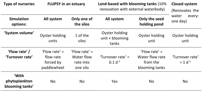
i) The nursery setup menu (Figure 3.3), is where the users enter their farm inputs such as flow rate (or turnover rate), water volume, water temperature and if the nursery includes blooming tanks. This model simulates the nursery system as a one compartment, which means for instance, if the nursery has blooming tanks the user should insert a) in the ‘System

volume’ the sum of the volume of the oyster holding unit and of the blooming tanks, b) in

the ‘Flow rate’or ‘Turnover rate’ the water exchange with the surrounding waterbody, and c) choose ‘Yes’ in “With phytoplankton blooming tanks’ box. Alternatively, that user can simulate only the oyster stock pond by inserting: a) in the ‘System volume’ the volume of that pond, b) in the ‘Flow rate’ or ‘Turnover rate’ the water exchange with the blooming

tanks, and c) choose ‘No’ in “With phytoplankton blooming tanks’ box. If the model is used

to simulate a FLUPSY in an estuary the user should insert: a) in the ‘System volume’ the volume of the FLUPSY, b) in the ‘Flow rate’or ‘Turnover rate’ the water flow rate forced by the paddlewheel into the entire FLUPSY, not of the individual silos, and c) choose ‘No’ in

(42)

22

Table 3.5 - Examples of nursery system definition for different types of nurseries (FLUPSY, Land-based with blooming tanks and closed systems).

Type of nurseries FLUPSY in an estuary Land-based with blooming tanks (10% renovation with external waterbody)

Closed system (Renovates the water every-one day) Simulation

options:

All system Only one of the silos

All system Only the seed holding pond

‘System volume’ _{Oyster holding} units

1 of the silos

Oyster holding unit + blooming

tanks

Oyster holding unit

‘Flow rate’ /

‘Turnover rate’ ‘Flow rate’ =flow rate forced by paddlewheel

‘Flow rate’ = Water flow rate into

one silo

‘Turnover rate’ = 0.1 d-1

‘Flow rate’ = Water flow rate

from the blooming tanks

‘Turnover rate’ = 1 d-1

‘With phytoplankton

blooming tanks’ No No Yes No No

Besides system definition, the nursery setup menu (Figure 3.3), is where the user inserts the average seed weight per grade. Default seed grades and average weights are provided but

the user can customize any of these by changing any of the boxes under ‘Oyster grades’ and ‘Seed weight’. ‘Choose food indicator’ allows the user to select his preferred food indicator for model inputs/outputs.

(43)

23 ii) In the output for food requirements menu (Figure 3.4), is presented the result about the food required for a given stock, which is expressed in the units chosen by the user in the previous

menu. The user should insert in this menu, below ‘Stock per grade (x103seeds)’ the amount

of seeds per grade. If the nursery includes blooming tanks then two outputs are shown that encompass a low and a high phytoplankton growth scenario (Figure 3.4).

Figure 3.4 - Model interface: model outputs for minimum external food concentration for a given stock. Full online interface available at http://seaplusplus4.com/oysterspatbud.html.

iii) In the output for optimum stock menu (Figure 3.5), are presented the results about maximum stock sustained, expressed as overall biomass and as number of seeds per grade, for two scenarios of available food. The model needs to ‘know’ the oyster biomass distribution per grade that the farmer aims, for instance 100% of small 0.04 g spat, or 50% of the biomass stock composed of small spat and 50% composed of 0.9 spat. The user can insert that input

under “Biomass % per grade” or the model calculates distribution per grade based on data

about ‘Stock per grade (x103seeds)’_{inserted in the previous menu (Figure 3.4). To test the}

(44)

24

Figure 3.5 - Model interface: model outputs for maximum stock that can be sustained for a given food input and considering a given stock distribution per grades. Full online interface

available at http://seaplusplus4.com/oysterspatbud.html.

iv) The advanced settings menu (Figure 3.6) allows the user to change the optimum food concentration for oyster filtration. That parameter ([Food]nursery) is detailed in the model description and it is not foreseen that the common user will have the data required to change this value. This menu also presents the model estimates for the clearance rate based on an allometric filtration rate function (Gerdes 1983a) and the temperature dependence effect that assumes optimum filtration rate for the Pacific oyster at 19˚C (Bougrier et al. 1995). If the nursery includes blooming tanks the user can change in this menu the phytoplankton growth rate values (Figure 3.6). The model allows the user to specify a low and a high phytoplankton growth rate to test the range of community net primary production scenarios

(45)

25

Figure 3.6 - Model interface: advanced biological parameters (user defined). Full online interface available at http://seaplusplus4.com/oysterspatbud.html.

Model limitations include:

i) Important effects that occur at a smaller scale like changes in the water flow rate due to oyster size/densities or tank shape are not simulated in the model.

ii) The option with blooming tanks assumes these are interconnected with the oyster holding tank, which together are the simulated unit. In this case the water flow is the water that enters from the outside (an adjacent ecosystem for instance) into the blooming tanks forced by tidal height or pumped.

iii) The salinity effects on filtration rate are not simulated thus it is assumed that water salinity is higher than 20.

RESULTS AND DISCUSSION

Model evaluation

(46)

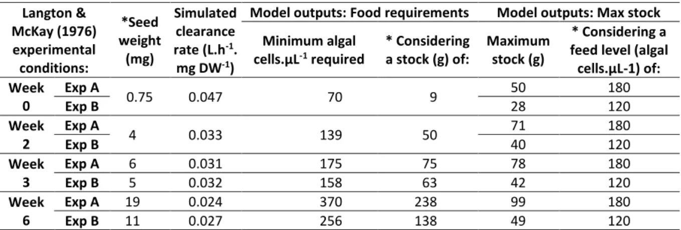
26 For a spat of 0.75 mg and a stock of approximately 9 g in the 250 L containers, which corresponds to the conditions at the beginning (week 0) of both experiments (A - high and B - low feed level) the estimated food requirement is around 70 algal cells. µL-1_{. For this spat weight and}

considering the two feed levels supplied, i.e. 180 algal cells. µL-1_{in Exp A and 120 algal cells. µL} -1_{in Exp B, the model estimates a maximum stock of 50 g and 28 g, respectively. The outputs of}

this model run indicate that at week 0 the feed supplied is much higher than the stock requirements.

The model outputs for the run that simulates week 2 indicate a food requirement around 139 algal cells. µL-1 _{for the 50 g stocked in the 250 L containers (spat around 4 mg). According to this}

simulation outputs, the feed level supplied in Exp A is still enough, nevertheless, oysters in the containers of Exp B are fed below the optimum.

In week 3 the feed level supplied is near the threshold in Exp A and does not meet the oyster requirements in Exp B, which according to the model outputs should be 175 and 158 algal cells. µL-1_{in Exp A and B, respectively. According to Langton & McKay (1976), the spat average weight}

in week 3 (6 and 5 mg in Exp A and B, respectively) already exhibit a slower growth for Exp B. In subsequent weeks the higher feed limitation experienced in Exp B (since week 2) is translated into lower weights, in week 4 spat weight is around 7.5 mg in Exp B compared with 13 mg in Exp A and by week 6 weight is around 11 mg in Exp B compared with 19 mg on Exp A (Langton & McKay 1976). These different growths measured in Exp A and B (Langton & McKay 1976) support the model predictions for food limitation. The model results also agree with the discussion of the experimental results by Langton & McKay (1976) according to which in the first 2 weeks the oyster spat are not feed limited.

Table 3.6 - Model outputs for Langton & McKay (1976) experiments. Langton & McKay (1976) experimental conditions: *Seed weight (mg) Simulated clearance rate (L.h-1_.

mg DW-1₎

Model outputs: Food requirements Model outputs: Max stock

Minimum algal cells.µL-1_required

* Considering a stock (g) of:

Maximum stock (g)

* Considering a feed level (algal cells.µL-1) of: Week

0

Exp A

0.75 0.047 70 9 50 180

Exp B 28 120

Week 2

Exp A

4 0.033 139 50 71 180

Exp B 40 120

Week 3

Exp A 6 0.031 175 75 78 180

Exp B 5 0.032 158 63 42 120

Week 6

Exp A 19 0.024 370 238 99 180

Exp B 11 0.027 256 138 49 120

(47)

27

Model application

The fact that the model implementation allows testing ranges of values for the external food concentration ([Food]External) and the phytoplankton growth rate (Growthphyt ) means that model

outputs provide a range of possible scenarios within which the nursery is operating. This facilitates model application into a given nursery whereby the user needs to provide the boundaries for this highly variable parameter (when dependent on food concentration in the surroundings). In extensive oyster nurseries, such seston concentration is unlikely to be monitored frequently. As such despite, the model simplification, it can still provide guidance for managing stock and food limitation in natural feeding oyster nurseries. These model functionalities contribute to support management of oyster nurseries. Namely, this model allows quantification of general rules of thumb regarding spat holding capacity for a given nursery. For instance, according with Helm & Bourne (2004) “Determining the biomass of spat

that can be held in a pond system is largely a matter of trial and error. A general rule is that 1

hectare surface area of shallow pond will support the production of between 1 and 3 tonnes

biomass of seed, depending on levels of algal productivity, over the course of a growing season.

This represents the maximum sustainable biomass that can be maintained with careful

management”. In order to apply the model for the described rule of thumb it is herein assumed: i) a water renovation with the external system of around 10%, ii) a system volume of about 10 000 m3_{corresponding to a surface area of 10 000 m}2_{for the blooming pond + 1 000 m}2_for

the stock pond and a 1 m water depth, iii) a water temperature around 19°C, iv) a phytoplankton concentration in the external waterbody within the range of about 0.5 - 2 µg Chl-a.L-1_{, v)}

phytoplankton growth rate that ranges between 0.5 d-1_{and 1.2 d}-1_{. The total biomass stock that}

(48)

28

Figure 3.7 - Model application for quantification of general rules of thumb about biomass stock that can be sustained by blooming ponds: a) model setup, b) model outputs considering spat

(49)

29 A wide range of other scenarios can be tested by any user in the online model (http://seaplusplus4.com/oysterspatbud.html) to better adjust a general rule of thumb to their own nursery conditions; for instance, and considering the abovementioned example, what are the changes regarding the stock biomass or number of seeds per grade that can be sustained due to lower or higher temperatures, typical of the local winter/summer? What if the local phytoplankton community growth rate is as low as 0.2 d-1_?

The inclusion in the model of a minimum concentration at the tanks that must be ensured to maximize ingestion ([Food]nursery) is one of the key elements to solve the mass balance at the

steady state. The practical implications of this assumption are that the model outputs provide i) the food requirements to ensure that minimum concentration in the nursery; considering a given water inflow, oyster filtration rate at a given stocking and seed weight, and if applicable phytoplankton natural production within the nursery; and, ii) the maximum biomass that can be stocked to ensure that minimum concentration at the nursery and thus ensure an optimized growth; considering a given food input, oyster seed weight and distribution among the oyster grades, and if applicable phytoplankton natural production within the nursery. The value adopted in the Pacific oyster model (3 mm3_.L-1_{as per rational explained in the section}_Model parameterization and validation for the Pacific oyster) was chosen from a set of 3 concentrations (0.5, 3, and 6 mm3_.L-1_{) tested by Tamayo et al. (2014). It is possible that within the interval}

between these values other solutions maximize ingestion. Further research should be developed to more accurately estimate the [Food]nursery. Given that other factors influence filtration

efficiency dependence on food concentration, such as the algae size (Winter 1978), further research should also include different feeds. For nurseries that provide cultivated algae they can improve their own model application by changing the [Food]nursery parameter (in

http://seaplusplus4.com/oysterspatbud.html) and inserting the value that best suits their own facility.

Nevertheless, the value adopted in the model parameterization for the Pacific oyster for the minimum food concentration that maximizes ingestion, i.e. [Food]nursery, (44 algae cells.µL-1 Table

3.3) is also in agreement with experiments by Langton & McKay (1976) whereby the growth was maximized for the feed supplied (120 or 180 algae cells.µL-1_{) with 6h interval which corresponds}

(50)

30

CONCLUSIONS

(51)

31

4. A dynamic model for oyster nurseries

In this section is presented a dynamic model for oyster nurseries, developed to simulate: (i) oyster spat individual growth, (ii) food availability within the farming system, and (iii) stock biomass. This model couples an individual bioenergetic model of oyster spat, upscaled to account the population dynamics of the overall stock, with a one-compartment mass balance model.

In the first sub-sections, a description of each model component (sub-section 4.1 - 4.4) is presented, as well as the results of model validation (subsection 4.5) and sensitivity analysis (subsection 4.6). In the last, are discussed the model developments (subsection 4.7).

4.1. Oyster spat individual bioenergetic model

4.1.1. Conceptual description

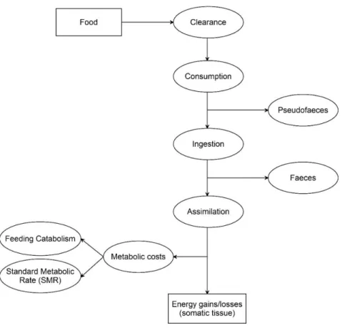
The oyster spat individual bioenergetic model (Figure 4.1) was developed to simulate the growth of Crassostrea gigas spat. The oyster energy balance was modeled based on NEB theory, which describes the net energy balance (NEB) as the difference between energy gains and energy losses (Gosling, 2004).

𝑁𝑒𝑡 𝑒𝑛𝑒𝑟𝑔𝑦 𝑏𝑎𝑙𝑎𝑛𝑐𝑒 (𝑁𝐸𝐵) = 𝑒𝑛𝑒𝑟𝑔𝑦 𝑔𝑎𝑖𝑛𝑠 − 𝑒𝑛𝑒𝑟𝑔𝑦 𝑙𝑜𝑠𝑠𝑒𝑠 (Eq. 4.1)

Energy gains result from food assimilation, the process that occurs after the consumption and ingestion of food. Generally, only a certain fraction of the food consumed is ingested, and the remaining fraction is rejected as pseudofaeces (Bayne, 2009). The food ingested is not all assimilated, being this process dependent, among others factors, on the quantity and quality of the food ingested (Bayne, 2017). The remaining food that is not assimilated is egested in the form of faeces. Energy losses are defined as the energy expended in metabolic activities, herein divided as standard metabolic rate and feeding catabolism. At this stage of model development excretion was not included in model formulation because it is a minor component of the oyster energy budget (Kobayashi et al., 1997; Bayne, 1999). Nevertheless, for a future use of the model, with the aim to calculate the oyster impact on the water/sediment biogeochemistry, this component must be included.