Article
Printed in Brazil - ©2009 Sociedade Brasileira de Química 0103 - 5053 $6.00+0.00
*e-mail: [email protected]; [email protected]
#Present address: Haagen-Smit Laboratory, California Air Resources Board, 9528 Telstar Avenue, El Monte, CA, 91731, USA.
Spark Ignition Vehicle Contributions to Atmospheric Fine Elemental Carbon Concentrations
in Coastal, Rural and Urban Communities using Polycyclic Aromatic Hydrocarbon
Tracers in the CMB Model Modified for Reactivity
Arantzazu Eiguren-Fernandez and Antonio H. Miguel*
,#Nanoparticle Chemistry Laboratory and Southern California Particle Center & Supersite, Institute of the Environment, University of California, 90095-1772, Los Angeles-CA, USA
Repartimos a parcela do componente de carbono elementar (CE) em PM2,5 atmosférico atribuível à emissões de veículos com ignição por faísca (SI) em amostras coletadas durante dois anos em doze comunidades no Sul da Califórnia, incluindo zonas costeiras, rurais e urbanas usando o Modelo de Balanço de Massa Química (CMB8) modificado para levar em conta a reatividade dos hidrocarbonetos policíclicos aromáticos (HPAs). Foram avaliadas as razões HPA/CE em amostras coletadas no túnel Caldecott para utilização como assinaturas das fontes. A reatividade dos HPAs que ocorre durante o transporte de aerossóis atmosféricos que pode afetar as estimativas de contribuição das fontes (ECF) durante o verão/primavera/outono foi considerada com o uso de constantes de decaimento medidas experimentalmente. Nossos resultados mostram que o benzo[ghi] perylene e o indeno[1,2,3-cd]pireno podem ser utilizados com sucesso como marcadores específicos de CE nas emissões por veículos com SI. A estimativa média da porção de CE atribuído pelo modelo à emissões provenientes de SI nessas comunidades foi de 39, 58 e 62%, respectivamente, durante o verão, primavera/outono, e inverno. Para todas as comunidades costeiras, as atribuições a veículos por SI representam cerca do dobro das estimativas para as áreas rurais e urbanas, antes de dezembro 2003 quando MTBE ainda era usado na California.
We apportioned the elemental carbon (EC) component of ambient PM2.5 attributable to emissions from spark ignition (SI) vehicles in samples collected over a three-year period in twelve Southern California communities, including coastal, rural, and urban areas using the chemical mass balance model (CMB8) modified for polycyclic aromatic hydrocarbon (PAH) reactivity. Selected PAH/EC ratios, measured in samples collected in the Caldecott tunnel were evaluated for use as fingerprints. PAH reactivity which occurs during atmospheric transport and affects the source contribution estimates during the summer/fall/spring months was accounted for using experimentally measured decay constants. Results showed that benzo[ghi]perylene and indeno[1,2,3-cd]pyrene can be used successfully as specific tracers of EC contributions from SI vehicles. The average EC portion of PM2.5 attributed by the model to SI emissions at these communities was 39, 58 and 62%, respectively, during the summer, spring/autumn, and winter. For all seasons, coastal community contributions represent about twice those found in the rural and urban inland communities, before December 2003 when MTBE was still in use in California.
Keywords: elemental carbon source apportionment, polycyclic aromatic hydrocarbons, spark ignition vehicles, PM2.5, chemical mass balance, MTBE
Introduction
Elemental carbon (EC) present in the atmospheric aerosol of urban and heavily industrialized locations constitutes a major component of the products of incomplete combustion (PICs) from liquid, solid and
gaseous fuels. Sources of EC in urban areas include spark ignition (SI) and compression ignition (CI) vehicular emissions, PICs generated from energy production and industrial combustion processes, tires, lubricating oil, railroad engines, boilers, aircraft, food cooking, biomass burning and many other processes that burn fossil fuel.1,2 In
the city of Los Angeles, fine elemental carbon (dp < 2.5 µm) account for 30-50% of the fine particle mass concentration.4
help improve our understanding of the impact of vehicular and other emissions sources on air quality12 and health
effects, and to monitor occupational exposure to SI and CI particulate matter.13
EC and the associated PAH components are ubiquitous in PICs14-16 and are mainly associated with fine, ultrafine,
and nanoparticles in the 10-32 nm size range.16-18
Research conducted in our laboratory has focused on the effects of fine and ultrafine (nano) particles present in ambient air on health effects.19 On going studies at
the Southern California Particle Center and Supersite (SCPCS) and the Southern California Environmental Health Sciences Center (SCEHSC) are aimed at evaluating possible correlations between EC and PAH content of the urban aerosol with indicators of in-vitro oxidative stress.20,21
Several high molecular weight PAHs (5-7 rings) associated with the atmospheric aerosol are considered carcinogenic and/or mutagenic. PAH profiles and emissions strength vary depending on their source.1,2,22,23
The ubiquity and similar emission sources of EC and PAHs creates a unique opportunity to use PAHs as source signatures in receptor modeling.15 One such model, the
Chemical Mass Balance (CMB) developed independently by Sheldon Friedlander in the early 70’s, has been widely used for source apportionment using a variety of inorganic and organic tracers.24-26 Beginning in 1986 researchers
suggested that certain PAHs may be used as tracers in receptor modeling.15
In this study we use the CMB8 model to estimate the EC component of PM2.5 attributable to spark ignition (SI) vehicles in twelve Southern California communities, during all seasons over a three-year period, by testing and selecting specific PAHs as tracers of SI vehicular emissions. The results are discussed in terms of: (i) the choice of PAH tracer; (ii) the effect of the location; (iii) the seasonal effect; and, (iv) the daily variability.
NIOSH 5040 procedure describe elsewhere.16,28 Details of the
PAH quantification procedure are described elsewhere.27,29
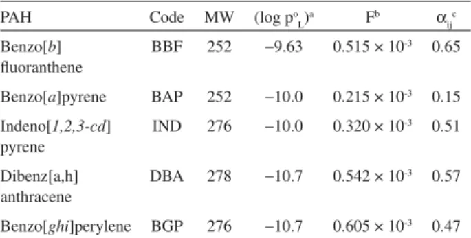
Samples for PAH quantification were extracted from the QFFs by ultrasonication using dichloromethane:acetonitrile (2:1, v/v) for 24 minutes (3×8 min). The extracts were filtered and their volumes reduced to ca. 100 µL at room temperature. Selective HPLC-Fluorescence was used to quantify 15 PAHs. The 5 PAHs tested as markers for the CMB8 model are listed in Table 1, along with their codes, molecular weight (MW), sub-cooled liquid vapor pressure, SI fractional concentration (source signature), and reactivity. PAH and EC profiles obtained in the Caldecott tunnel in 1996, and used in the present study, are reported elsewhere.1
Chemical mass balance model
The chemical composition of the emissions from individual sources can be used to estimate source contributions to atmospheric samples taken at receptor air monitoring sites.30,31 The CMB model used in this study,
together with the instruction, was obtained from the USEPA web site http://www.epa.gov/scram001/tt23.htm.
Table 1. PAH code, molecular weight, sub-cooled vapor pressure (atm), SI signatures and experimentally determined PAH reactivity factors
PAH Code MW (log po
L)
a Fb α
ij c
Benzo[b] fluoranthene
BBF 252 −9.63 0.515 × 10⁻³ 0.65
Benzo[a]pyrene BAP 252 −10.0 0.215 × 10⁻³ 0.15
Indeno[1,2,3-cd] pyrene
IND 276 −10.0 0.320 × 10⁻³ 0.51
Dibenz[a,h] anthracene
DBA 278 −10.7 0.542 × 10⁻³ 0.57
Benzo[ghi]perylene BGP 276 −10.7 0.605 × 10⁻³ 0.47
In this model, the total ambient mass concentration Ci of a specie i measured at a receptor site is expressed mathematically as:
Ci = Σ(Sj Fij) + Ei (1)
where Fij is the fraction of specie i in the emissions from source j, Sj is the total mass concentration contributed by source j at the receptor site, and Ei represents random errors in the measurement of Ci and Fij or unaccounted-for sources. As PAHs are know to react during atmospheric transport, and to overcome the implicit inert species assumption in the above equation, a reactivity factor, α, is included in the equation. The revised mass balance equation24 is given by:
Ci = Σ(Sj Fijαij) + Ei (2)
where Ci, Fij and Sj have the same meaning as the parameters used in equation 1, αij is the decay factor of specie i for source j expressed as the ratio of receptor concentration to the source concentration normalized to mass:
αij = 1/(1+kijτj) (3)
where kij is the decay constant for specie i, and τj is the average residence time in the atmosphere.
To account for decay during atmospheric transport, we reduced our individual PAH source signatures (Table 1), by experimentally calculated decay losses observed for Caldecott tunnel samples collected on filters subsequently exposed to particle-free Los Angles ambient air, under prevailing atmospheric conditions for a period up to 100 h.32
Results and Discussion
Choice of PAH tracers
The emission profiles of ten PAHs measured in Bores 1 and 2 of the Caldecott tunnel1 from SI and CI emissions,
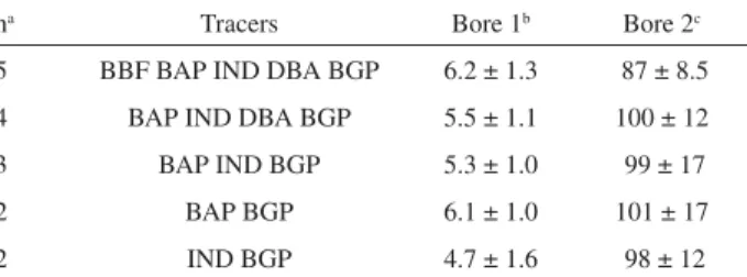
including fluoranthene, pyrene, benzo[a]anthracene, chrysene, benzo[b]fluoranthene, benzo[k]fluoranthene, benzo[a]pyrene, indeno[1,2,3-cd]pyrene, dibenz[a,h] anthracene and benzo[ghi]perylene are shown in Figure 2. It is clear that the PAHs with lower MW (FLT, PYR, BAA and CRY) are not suitable choices, as the fraction of EC from CI emissions are larger or close to those from SI emissions. For this reason, we tested different combinations of the remaining PAHs (Table 2) using the CMB model with the fractional concentrations listed in Table 1. As no reaction occurs at the tunnel no reactivity coefficient was included in these calculations.
Bore 1 of the Caldecott tunnel represents a mixed fleet of SI and CI, while Bore 2 is only open to SI traffic. Samples from Bore 1 were collected during time periods when the
Figure 1. Location of six of the twelve Southern California Children’s Health Study communities in coastal, and inland urban and rural areas. Atascadero, not sown in the map, is located ca. 70 Km north of Santa Maria.
tunnel fleet traffic mix is obtained using IND and BGP as tracers, respectively 4.7% and 98% of EC contributions in Bores 1 and 2 (Table 2).
Other PAH tracer combination that yielded accurate SCEs included BAP and DBA, but were discarded as candidates for source apportionment of field samples because BAP is the most reactive PAH in the group, and ambient concentrations of DBA are in general very low. The use of BGP as a vehicular tracer in the CMB model has been reported previously.30,33 Thus, in the present study, IND and
BGP were used as tracers to estimate the EC contributions to PM2.5 attributed by the model to SI emissions in coastal, rural inland and urban inland communities in Southern California.
or no industrial emission sources. Atascadero, a community highly impacted by traffic from the nearby freeway, showed the highest all-season average contribution (62.3%), while Lake Arrowhead, a rural community located at high altitude, had the lowest all-season average contribution of all sites (16.5%). The relatively lower SCEs observed in Riverside and Miraloma, located the furthest downwind from the metropolitan Los Angeles, suggest a larger impact from other EC sources such as CI emissions, local industries and atmospheric transport. It is noteworthy to mention that, over the last decade, the urban inland communities of Upland, Mira Loma, and Riverside are home to numerous warehouse distribution centers serviced by thousands of heavy-duty diesel trucks (CI) each day.
Table 3. Estimates of SI vehicles emission contributions to %EC in PM2.5
Spring/fall Summer Winter All-season site average
Coastal communities
Lompoc 30.6 ± 28 55.4 ± 30 49.1 ± 21 45.0 ± 26
Santa Maria 81.4 ± 20 30.6 ± 17 49.1 ± 30 53.7 ± 22
Atascadero 61.9 ± 26 50.6 ± 15 74.3 ± 23 62.3 ± 21
Long Beach 56.9 ± 35 18.3 ± 9.1 73.9 ± 39 49.7 ± 27
Season average 57.7 ± 21 38.7 ± 17 61.6 ± 14 52.7 ± 17
Rural inland communities
Lancaster 36.0 ± 37 9.70 ± 10 n/a 22.9 ± 23
Lake Arrowhead 26.7 ± 24 3.43 ± 2.7 19.4 ± 19 16.5 ± 15
Lake Elsinore 45.4 ± 34 19.3 ± 8.8 24.2 ± 25 29.6 ± 23
Alpine 57.5 ± 27 17.6 ± 13 17.2 ± 11 30.8 ± 17
Season average 41.4 ± 13 12.0 ± 7.4 20.3 ± 3.6 24.9 ± 8.0
Urban inland communities
San Dimas 35.0 ± 15 16.9 ± 9.4 37.5 ± 19 29.8 ±14.5
Upland 16.4 ± 10 19.3 ± 15 36.6 ± 23 24.1 ± 16.0
Mira Loma 22.6 ± 13 26.5 ± 14 46.8 ± 39 32.0 ± 22.0
Riverside 24.0 ± 16 16.5 ± 8.2 34.2 ± 22 24.9 ± 15.4
Season average 24.5 ± 7.7 19.8 ± 4.6 38.8 ± 5.5 27.7 ± 6.0
Seasonal variability
Samples were arranged in three different seasons: spring/autumn, summer, and winter, depending on the average ambient temperature. Average seasonal contributions for each community and group are shown in Table 3. The contribution by SI emissions in the costal communities varies from 18.3% in Long Beach during the summer to 81.4% in Santa Maria during spring/fall. For rural inland communities SCEs vary between 3.43% for Lake Arrowhead during summer, and 57.5% for Alpine during spring/fall. Among the urban inland communities Miraloma was the highest with SI contributing up to 46.8% during winter; Riverside and Upland presented the lowest contributions with ca.16.5% during summer and spring/ fall, respectively.
In general, coastal and urban inland communities showed higher SI contribution during the winter period, while spring/fall showed higher contributions for the rural inland communities.
Seasonal difference between coastal and inland sites in southern California has been reported and explained by Gray et al.,4 and our results are similar to previous
estimates reported by Manchester-Neesvig et al.,34 and
Riddle et al.35 who reported a 14-21% contribution to
PM0.1 EC by gasoline combustion (SI) products and motor oil combustion products (5-6%). The observed differences in the estimated SI contribution to EC during the three seasons may have resulted from several factors, including: (i) meteorology, (ii) a decrease in the number of SI on the road during summer, (iii) higher than-accounted-for photochemical PAH reactions during spring and summer, and (iv) increased emissions from sources that also contribute to atmospheric BGP (e.g. fire places) when the ambient temperature becomes cooler as winter approaches. In the winter, the net air mass movement is toward the off-shore direction, placing sites like Long Beach downwind of the city when wind speeds are slow and early morning surface temperature inversions are common. During the summer, the prevailing wind direction is reversed and strong on-shore flow transports the aerosol masses from the Los Angeles Basin deep into the inland communities and mountains. Vehicular cold starts during winter are known to increase exhaust aerosol emissions, a factor that may contribute significantly to the higher SCE values estimated for the urban sites during spring/fall and winter. Although one might think that during winter wood burning may be an important source of BGP, the contribution of this source to the total BGP burden is not significant.36
While newer CI engines and improved diesel fuels may have reduced EC levels found a decade ago, the lowest
EC estimates attributable to SI emissions indicate that CI emissions remain the major source of fine particle EC emissions.
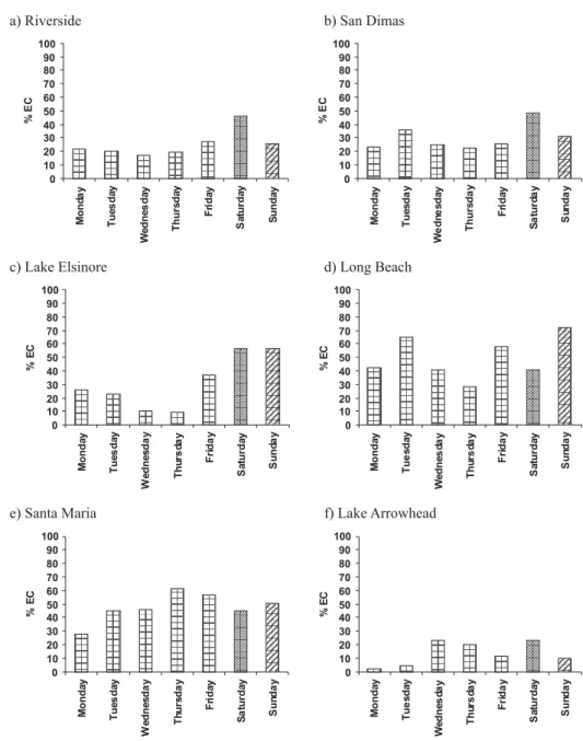
Daily variability
Sample collection occurred every 8th day, allowing the evaluation of possible day-of-the-week effects on the SI contribution to EC from SI emissions (Figure 3). In general, communities highly impacted by local commuters, or significant daily activities such as Santa Maria and Long Beach, did not show significant differences between weekdays and weekends (Figure 3). In communities such as Lake Elsinore, or communities impacted by weekdays HDD shipment traffic such as Riverside and San Dimas, the contribution of SI vehicles to the EC burden appeared to be more important during weekends.
Conclusions
The CMB model has been applied to estimate spark ignition (SI) vehicle emissions to the atmospheric elemental carbon contained in PM2.5 using IND and BGP as specific tracers. Our estimated season-averaged fraction of EC (19.8%) attributable by the model to light duty vehicles during the summer months in urban inland communities agrees well with the 14-21% found for ultrafine PM reported by Riddle et al.35 for summer measurements using
benzo(ghi)perylene+coronene as tracers of SI emissions downwind of a roadway in San Diego, California, located
ca. 120 km to the south of Los Angeles. We conclude that, at the communities studied and communities with similar major EC emission sources, BGP and IND may be used as tracers in the CMB model, corrected for reactivity during the spring/fall and summer seasons, to apportion the EC component attributable to spark ignition emissions. The model also showed both seasonal and spatial variability based on traffic intensity and geographical conditions. Regional off-shore transport during warmer seasons and on-shore transport during the winter months may have an effect in the extent of EC apportionment to SI emissions. Daily variability appeared to be only important in communities also impacted by CI emissions, before the ban of MTBE.
Acknowledgments
Figure 3. Average daily variability of %EC emissions from spark ignition at different locations.
study,27 Mahnaz Hakami for her help in the preparation of
sample matrices and carbon analysis, Richard Kamens, Joellen Lewtas, Pablo Cicero-Fernandez, and Susanne Hering, for their insights and helpful suggestions during the course of this study. This research was supported by the Southern California Particle Center and Supersite (USEPA Grants #R827352-01-0 and CR-82805901) and the NIEHS Center Grant (SP30ES07048-02). Although the research described in this article has been funded wholly or in part by the United States Environmental Protection Agency, it has not been subjected to the Agency’s required peer and policy review and therefore does not necessarily reflect the views of the Agency and no official endorsement should be inferred.
References
1. Miguel, A. H.; Kirchstetter, T. W.; Harley, R. A.; Hering, S. V.;
Environ. Sci. Technol.1998,32, 450.
2. Schauer, J. J.; Kleeman, M. J.; Cass, G. R.; Simoneit, B. R. T.;
Environ. Sci. Technol.2001,35, 1716.
3. Miguel, A. H.; Sci. Total Environ. 1984,36, 305.
4. Gray, H. A.; Cass, G. R.; Huntzicker, J. J.; Heyerdahl, E. K.;
Rau, J. A.; Environ. Sci. Technol.1986,20, 580.
5. Schauer, J. J.; Rogge, W. F.; Hildemann, L. M.; Mazurek, M.
A.; Cass, G. R.; Atmos. Environ.1996,30, 3837.
6. Gray, H. A.; Cass, G. R.; Atmos. Environ. 1998,32, 3805.
7. Allen, A. G.; Miguel, A. H.; Environ. Sci. Technol.1995,29,
8. Cooke, W. F.; Wilson, J. J. N.; J. Geophys. Res-Atmospheres
1996,101, 19395.
9. Charlson, R. J.; Heintzenberg, J.; Aerosol Forcing and Climate,
Wiley: New York, 1995.
10. (IPCC), I. P. o. C. C.; Climate Change 1994: Radiactive
Forcing of Climate Change and an Evaluation of the IPCC
IS92 Emission Scenarios; Cambridge University Press: New York, 1994.
11. Venkataraman, C.; Habib, G.; Eiguren-Fernandez, A.; Miguel,
A. H.; Friedlander, S. K.; Science2005,307, 1454.
12. (NRC), N. R. C.; Protecting Visibility in National Parks and
Wilderness Areas; National Academy Press: Washington D.C., 1993.
13. Schauer, J. J.; J. Exp. Anal. Environ. Epidemiol.,2003,13, 443.
14. Oanh, N. T. K.; Reutergardh, L. B.; Dung, N. T.; Environ. Sci.
Technol. 1999,33, 2703.
15. Daisey, J. M.; Cheney, J. L.; Lioy, P. J.; J. Air Pollut. Control
Assoc. 1986,36, 17; Rocha, G. O.; Lopes, W. A.; Pereira, P. A. P.; Vasconcellos, P. C.; Oliveira, F. S.; Carvalho, L. S.;
Conceição, L. S.; de Andrade, J. B.; J. Braz. Chem. Soc.2009,
4, 680.
16. NIOSH; Elemental Carbon (Diesel Particulate): Method 5040;
4th ed.; NIOSH: Cincinnati, 1996.
17. Miguel, A. H.; Eiguren-Fernandez, A.; Sioutas, C.; Fine, P. M.;
Geller, M.; Mayo, P. R.; Aerosol Sci. Technol.2005,39, 415.
18. Mastral, A. M.; Callen, M. S.; Environ. Sci. Technol. 2000,34,
3051.
19. Peters, J. M.; Avol, E.; Gauderman, W. J.; Linn, W. S.; Navidi, W.; London, S. J.; Margolis, H.; Rappaport, E.; Vora, H.; Gong, H.;
Thomas, D. C.; Am. J. Respir. Crit. Care Med. 1999, 159, 768.
20. Li, N.; Hao, M. Q.; Phalen, R. F.; Hinds, W. C.; Nel, A. E.; Clin.
Immunol.2003,109, 250.
21. Li, N.; Sioutas, C.; Cho, A.; Schmitz, D.; Misra, C.; Sempf, J.;
Wang, M. Y.; Oberley, T.; Froines, J.; Nel, A.; Environ. Health
Perspect. 2003,111, 455.
22. (US-EPA), U. S. E. P. A.; Air Quality Criteria for Particulate
Matter, Second External Review Draft, US-EPA, 2001. 23. Schauer, J. J.; Kleeman, M. J.; Cass, G. R.; Simoneit, B. R. T.;
Environ. Sci. Technol. 1999,33, 1578.
24. Li, C. K.; Kamens, R. M.; Atmos. Environ., Part A1993, 27, 523.
25. Schauer, J. J.; Kleeman, M. J.; Cass, G. R.; Simoneit, B. R. T.;
Environ. Sci. Technol. 2002,36, 1169.
26. Fujita, E. M.; Watson, J. G.; Chow, J. C.; Lu, Z. Q.; Environ.
Sci. Technol. 1994,28, 1633.
27. Eiguren-Fernandez, A.; Miguel, A. H.; Froines, J. R.; Thurairatnam,
S.; Avol, E. L.; Aerosol Sci. Technol. 2004, 38, 447.
28. Birch, M. E.; Cary, R. A.; Aerosol Sci. Technol. 1996,25, 221.
29. Eiguren-Fernandez, A.; Miguel, A. H.; Polycyclic Aromat.
Compd.2003,23, 193.
30. Cass, G. R.; McRae, G. J.; Environ. Sci. Technol. 1983, 17, 129.
31. Friedlander, S. k.; Environ. Sci. Technol. 1973,7, 235.
32. Miguel, A. H.; Deandrade, J. B.; Hering, S. V.; Int. J. Environ.
Anal. Chem. 1986,26, 265.
33. Venkataraman, C.; Friedlander, S. K.; Environ. Sci. Technol.
1994,28, 563.
34. Manchester-Neesvig, J. B.; Schauer, J. J.; Cass, G. R.; J. Air
Waste Manage. Assoc. 2003,53, 1065.
35. Riddle, S. G.; Robert, M. A.; Jakober, C. A.; Hannigan, M. P.;
Kleeman, M. J.; Environ. Sci. Technol. 2008,42, 6580.
36. Fine, P. M.; Cass, G. R.; Simoneit, B. R. T.; Environ. Sci.
Technol. 2001,35, 2665.
37. Calvert, J. G.; R., A.; Becker, K. H.; Kamens, R. M.; Seinfeld,
J. H.; Wallington, T. J.; Yarwood, G.; The Mechanisms of
Atmospheric Oxidation of Aromatic Hydrocarbons, Oxford University Press: New York, 2002.
Received: November 24, 2008