Density Functional Theory Method for Non-Equilibrium Charge
Transport Calculations: TRANSAMPA
Frederico D. Novaes, Antˆonio J. R. da Silva, and A. Fazzio
Instituto de F´ısica, Universidade de S˜ao Paulo, CP 66318, 05315-970, S˜ao Paulo, SP, Brazil
Received on 6 May, 2006
We describe a procedure to calculate charge transport properties across a nanosystem. This scheme is based on a Green’s Function formalism to treat a non-equilibrium problem, coupled to the Density Functional Theory to describe the electronic structure. As an illustration, we perform calculations for the charge transport across a (5,5) carbon nanotube with a vacancy.
Keywords: Charge Transport; Density Functional Theory; Non-Equilibrium Green’s Function
I. INTRODUCTION
In the past few years it has been possible to measure the charge transport across nanometric systems, such as carbon nanotubes, metallic nanowires, and molecules[1]. All these systems have the same basic physical picture, with a central scattering region connected to a certain number of leads. Even though many fundamental concepts related to the understand-ing of how charge flows in such small systems are already well established[2], there are still quite a few challenges if one wants to quantitatively calculate a property such as anI×V curve.
Any theory with this predictive power should obey a num-ber of requirements: i) a reliable description of the electronic structure properties of the atoms in the scattering region; ii) the treatment of the leads in the same footing as the scatter-ing region; iii) it should have no adjustable parameters; iv) the self-consistent calculation of the charge redistribution within the scattering region due to the application of a voltage bias; v) it should do all this for a variety of different systems. Al-beit with some drawbacks, as discussed later on, the Density Functional Theory Non-Equilibrium Green’s Function (DFT-NEGF) approach[3–5] to charge transport calculations comes very close to satisfying a good number of these requirements. One could say that DFT[6] is today the standard approach for ab initio electronic structure calculations of medium to large systems, including molecules, bulk solids, surfaces, nano-systems, etc. There are theorems that guarantee its solid foundation as an exact theory, in principle. To perform prac-tical calculations, approximations are necessary. There are, however, excellent schemes that lead to reliable and predic-tive results for properties such as structural geometries, vi-brational frequencies, energy barriers, and heats of reactions. All these properties are obtained from the total energy of the system, which is guaranteed to be a minimum of the density. The usual implementations of the DFT do not directly use an approximation of the total energy as a functional of the den-sity, but employ a more reliable scheme that introduces an auxiliary set of one-particle-like equations, the Kohn-Sham (KS) equations. This scheme is introduced in order to cal-culate with acceptable accuracy the major part of the kinetic energy. It is important to stress that although the majority of the DFT calculations employ these single-particle KS
equa-tions, this does not mean that DFT is a mean-field theory. DFT for equilibrium situations is a full many-body calcula-tion, and the only approximation is contained in the so-called exchange-correlation functional.
Even though these KS equations have an auxiliary role in the theory (the total charge density is obtained from the KS orbitals), their eigenvalues, i.e. the KS spectrum, are usu-ally used as an estimate of the true excitation spectrum of the system, and experience shows that this is in general a good approximation, except for an underestimation of the gap in semiconductors and insulators (or the gap between the highest occupied molecular orbital (HOMO) and the lowest unoccu-pied molecular orbital (LUMO) in molecules). Moreover, the KS orbitals also provide a good approximation for the quasi-particle orbitals.
In DFT-NEGF the use of DFT to describe the electronic structure of the problem does not have the same solid foun-dation as in equilibrium calculations. The idea is to use the KS orbitals and eigenvalues, or in other words, the KS tonian, as a good description for the scattering-region Hamil-tonian as well as for the leads HamilHamil-tonian and for the cou-pling between the leads and the scattering region,i.e., the sys-tem Hamiltonian is written as
H=
∑
In
εInc†IncIn+
∑
α
εαd†αdα+
+
∑
Inα
(VIn,αc†Indα+c.c), (1)
wherec†In(cIn)creates (destroys) an electron in a KS orbital
with KS energyεIn, for theIlead (I=L,R), anddα†(dα) cre-ates (destroys) an electron in a scattering region KS orbital with KS energyεα. The indicesnandαgenerically represent all the necessary quantum numbers to label the eigenstates. As it can be seen, DFT is used here in a mean-field like spirit. There will be, therefore, limitations associated with this ap-proximation. However, there is the enormous gain that the whole system is treated fully ab initio with a powerful method, and realistic systems can be described at an atomistic level.
a vacancy.
II. METHOD
A. Conductance Calculation
A given potential biasV applied between two electrodes will cause a currentIto flow across the system.
The relation betweenI andV is provided by the conduc-tanceG, given by
G= I
V. (2)
A general expression for the currentI has been obtained by Meir and Wingreen [9] within the Non-Equilibrium Green’s Function formalism[10], where arbitrary interactions can oc-cur within the scattering region. For the particular situation where the Hamiltonian describing the scattering region has a non-interacting form, the formula for the current is given by
I=e h
Z ∞
−∞T(E) ¡
nLFD(E)−nRFD(E)¢
dE, (3)
whereT(E)is the transmission function [4, 5, 9],
T(E) =Tr[ΓLGr(E)ΓRGa(E)], (4)
with,
ΓL(R)(E) =i
³
Σr
L(R)(E)−
¡
Σr L(R)(E)
¢†´
, (5)
ΓL(R)(E) =−2Im[ΣrL(R)(E)], (6)
and we have assumed time reversal symmetry. In the above formulas,nL(R)FD (E)is the Fermi-Dirac distribution function for the left (right) electrode, and the definitions and discussion re-garding all the Green’s functions and self-energies used above will be presented in the next section.
In the limitV →0,T→0, where T is the temperature, we assume a linear regime, with a mean valueT(E)¯ in thesmall range of integration in (3),
I→e
hT(E)¯
¡
EFL−EFR¢=e 2
hT(E)V¯ , (7) whereEFL(R)is the left (right) chemical potential. The conduc-tance may, thus, be evaluated with an equilibrium calculation,
G=2e 2
h T(EF), V →0,T→0, (8) considering spin degeneracy[11].
The main goal of the present implementation, as in pre-vious ones [3–5, 12], is to devise a scheme to calculate the above Green’s functions, and thus the current, from a fully
ab initio method. We then use a DFT formalism. As al-ready mentioned, in DFT the total energy and other properties are obtained via auxiliary one-particle equations, the Kohn-Sham equations. Both the resulting one-particle orbitals as well as the energies have no formal use in DFT. Albeit this caveat, they are usually considered to be a good approxima-tion to the true quasi-particle wave-funcapproxima-tions and excitaapproxima-tion spectrum, respectively. Note, however, that there is the well known gap-problem within the DFT[13], as well as problems with the current exchange-correlation potentials, such as self-interaction errors[13].
In a mean-field spirit, the DFT formalism is used together with the NEGF to calculate the Green’s functions and then the current. In the DFT formalism, the potential in the Kohn-Sham Hamiltonian depends on the electronic density. Thus, there is the need to solve these non-linear equations self-consistently. For equilibrium situations, the density matrix is traditionally obtained via the Kohn-Sham orbitals, through an appropriate application of either open (finite systems) or pe-riodic boundary conditions, plus the self-consistent solution of the Kohn-Sham equations. The procedure presented below describes how to obtain the density matrix self-consistently, for both equilibrium and non-equilibrium situations, using Green’s functions and open boundary conditions, for infinite systems.
The model consists of inserting two (large) electrodes (leads), to the left and to the right of a (nanoscale) region whose transport properties will be investigated (see Fig. 1). This partitioning in different regions, and the possibility to work with finite size matrices to simulate an open, non-periodic infinite system, is made possible by the use of lo-calized basis sets[4]. Here we use all the developments that have already been implemented in the SIESTA code, in par-ticular, localized atomic orbitals (which are strictly zero be-yond certain cutoff radii). We then extend the code to be able to simulate open, non-periodic systems.
FIG. 1: Scheme for the geometrical structure used in the transport calculations, showing the left lead (L) and the right lead (R) connect-ing the scatterconnect-ing (central) region (C). The system displayed here is a (5,5) carbon nanotube, and there is a single vacancy in the scattering region. This procedure of splitting the system in three regions is a general feature of the DFT-NEGF implementation.
B. Green’s function and the Density matrix
smallest group of neighboring atoms, instead of infinite slabs (see Fig. 2).
FIG. 2: Illustration of a small region of a (5,5) carbon nanotube bulk, containing 3 principal layers (PL, see text for details), shown in al-ternate shades of gray. Note that each PL contains three bulk unit cells, composed of 20 carbon atoms. The size of the PLs is chosen such that, due to the strictly localized character of the basis functions, there is only coupling between nearest neighboring PLs. For exam-ple, in the (5,5) nanotube shown, the leftmost PL does not couple to the rightmost PL.
We may thus consider to be working with tri-diagonal ma-trices, where thediagonalelements are matrices representing a PL. Then, for an infinite system, a Hamiltonian (or Overlap -S) matrix, will have the general form,
H=
. .. ... ... ... ... . .. · · · H0,0 H0,1 0 0 . . .
· · · H1,0 H1,1 H1,2 0 . . .
· · · 0 H2,1 H2,2 H2,3 . . .
· · · 0 0 H3,2 H3,3 . . . . .. ... ... ... ... . ..
(9)
where each element of the above matrix is itself a matrix whose size is the number of basis set elements contained in a PL. For example, in the example shown in Fig. 2, each PL has three bulk unit cells. Each bulk unit cell has 20 C atoms, so that there are 60 C atoms in a PL. If we use 13 basis functions for each C atom, each PL has a total of 780 basis function, and this is the dimension of each one of these block matrices. All theHI,Imatrices are identical, as are also theHI,JPL coupling
matrices.
When we use Greek letters as matrix indices, they represent specific atomic orbitals, and when L, R or C are used, they represent whole regions, the left or right electrodes (that are infinite) and the central (scattering) region, respectively. Bold letters symbolize matrices. Here we emphasize that the term Bulkmeans a periodic infinite system, and that it may not be a three dimensional one (as the example in Fig. 2, an infinite carbon nanotube that simulates the leads).
1. Equilibrium Situation
We start by considering how to solve a DFT problem for an open system, still in an equilibrium situation, i.e., when there is no potential bias between the left and right leads.
The usual approach for this type of situation is to use a su-percell approximation, where the “defect” region, plus a bulk buffer region, are periodically repeated in space. This artifi-cial periodicity usually provides quite accurate results. Care must, however, be taken in order to prevent (or at least re-duce) that the spurious interactions between images affect the final results/conclusions. In some cases, such as carbon nan-otubes, we have observed that it is quite hard to reduce these interactions to an acceptable level, since the periodically re-peated defects introduce a periodic potential that opens up gaps at every band degeneracies at the Brillouin zone bound-aries, which are mainly due to the zone folding due to the su-percell approximation. In cases like these, the use of Green’s functions to exactly treat an open boundary situation is quite advantageous. This type of application is a quite general use of Green’s functions[15, 16], and is not particularly related to NEGF. Moreover, the construction outlined below can be used as part of a procedure to obtain the transmittance in the linear response regime.
We start with the formal definition of the retarded Green’s function [15],
¡
E+ˆ1−Hˆ¢ˆ
Gr(E) =ˆ1, (10)
where
E+= lim
δ→0+E+iδ. (11)
Representing the set of basis orbitals by{|φµi}, theDualset,
{|φµi}, is such that
hφµ|φ
νi=δµν. (12)
Using the completness relation,
ˆ1=
∑
µ
|φµihφµ|=
∑
µ|φµihφ
µ|, (13)
we obtain the matrix form of (10),
∑
λ ¡
E+Sµ,λ−Hµ,λ¢Grλ,ν(E) =δµ,ν, (14)
with
Sµ,ν=hφµ|φνi, (15)
Hµ,ν=hφµ|HˆKS|φνi, (16)
Grµ,ν(E) =hφµ|Gˆr(E)|φνi, (17) where ˆHKS is the Kohn-Sham Hamiltonian. The matricesH
andSare obtained using the SIESTA code[7], which is based on DFT.
ˆ
HKS|ψii=Ei|ψii, (18)
one solves the generalized eigenvalue problem,
∑
λ
Hµ,λcλi =Ei
∑
λ
Sµ,λcλi (19)
with
cλi =hφλ|ψii. (20)
From this, one can obtain the density matrix,
ρµ,ν=
∑
i
cµicνi∗nFD(Ei), (21)
wherenFD(E)is theFermi-Diracfunction. Since we now
par-tition the system in three regions, left and right infinite elec-trodes and a central (scattering) region, this is no longer pos-sible.
SinceGrµ,ν(E)can be written in aspectralform[4, 15],
Grµ,ν(E) =
∑
i
cµicνi∗ E+−Ei
, (22)
and using the relation (we consider thatx0lies in the interval [a,b]), we have
Zb
a
f(x)
x−x0±iδ dx=PV
·Z b
a
f(x) x−x0dx
¸
∓iπf(x0), (23) with
PV
·Zb
a
f(x) x−x0
dx
¸
=lim
δ→0
·Z x0−δ
a
f(x) x−x0
dx+
Z b
x0+δ
f(x) x−x0
dx
¸ ,
(24)
which is theCauchy principal value. We see that Z ∞
−∞ ¡
Grµ,ν(E)−Gaµ,ν(E)¢
nFD(E)dE=−2iπρµ,ν, (25)
whereGaµ,νis the advanced (matrix) Green’s function, defined in similar way as the retarded function, with E+ being re-placed byE−,
E−= lim
δ→0+E−iδ. (26)
Considering that the system has time reversal symmetry, the retarded and advanced matrices are related,
Ga(E) =¡
Gr(E)¢†
=¡
Gr(E)¢∗
, (27)
and we obtain the (well-known) expression that is used to cal-culate the equilibrium density matrixρC,C,
ρC,C=−
1 πIm
·Z ∞
−∞G
r
C,C(E)nFD(E)dE
¸
. (28)
In this way, we see that this procedure is entirely equivalent to the usual scheme where one first obtains the Kohn-Sham orbitals, and from them the density matrix. However, we can now obtain the density matrix of an open system.
2. Non-Equilibrium
If the system is in non-equilibrium, the expression to ob-tain the density matrix is more involved than equation (28). We then use the NEGF technique, which is developed follow-ing the contour path formalism to calculate the expectation values of time dependent operators[17], in particular, Green’s Functions, like the retarded and correlation (or lesser) Green’s Function, which are defined, respectively, as
Gr(x,x′) =−iθ(t−t′)h[ψˆH(x),ψˆ†H(x′)]+i, (29)
G<(x,x′) =ihψˆ†H(x′)ψˆH(x)i, (30)
wherex≡(r,t), and ˆOH(t) is a general operator ˆO in the
Heisenberg picture. More details can be found in references [18, 19]. For a derivation of the equations in the case of a representation in a non-orthogonal basis set, see the work of Thygesen [20].
It is established that, if thecentral(scattering) region is in contact with two reservoirs that do not interact directly with each other, but that are each one in thermodynamic equilib-rium characterized by a different electrochemical potential, the density matrix of the central region can be obtained by
ρC,C=
1 2π
Z
GCr,C(E)¡
nLFD(E)ΓL(E)+
nRFD(E)ΓR(E)¢GCa,C(E),
(31)
where all the matrices have the size of the number of basis elements of the central region. All the matrices above will be properly defined below.
C. Retarded Green’s Function of the Central Region
Now we need a scheme to calculate the retarded Green’s function of the central region, and the self-energies that repre-sent the coupling to the leads. Due to the fact that a localized set of basis functions is used, the matricesHandS can be written in tri-diagonal form. This makes it possible to obtain an expression for the retarded matrix Green’s function for the central region[4]. Note that the left and right electrodes do not have a direct interaction, that isHL,R=SR,L=0 [21]. We
hA,B=E+SA,B−HA,B(AandB=L,C,R). (32)
It is then possible to show that the retarded Green’s function of the central region can be written as [4]
GCr,C(E) =¡
hC,C−ΣrL(E)−ΣrR(E)
¢−1
, (33)
where the self-energies are defined as
Σr
L(E) =hC,LgrL,L(E)hL,C, (34)
ΣrR(E) =hC,RgRr,R(E)hR,C. (35)
These self-energies depend on the leads Green’s functions,
grA,A(E) =¡
E+SA,A−HA,A
¢−1
(A=L,R). (36)
This scheme would seem impractical, since equation (36) in-volves, in principle, the inversion of a semi-infinite matrix. However, the inter-block matriceshC,L,hL,C,hC,R andhR,C,
are non zero only for a finite number of elements. It is then necessary to find only a finiteportionofgL,LandgR,R, called
the surface Green’s function. In this implementation we have used the recursive algorithm described in Ref. [14], although other options can also be employed[12].
D. Density matrix of the scattering region
Either in the case of equilibrium or non-equilibrium, the density matrix of the central region is obtained via an integra-tion over the energy variable.
The importance of the expression (28) is that, for a com-plex variable Z in place of the realE,Gr(Z)is analytic for
Im[Z]>0, and that this function is smoother for complex val-ues ofZ. This integral can then be evaluated using a com-plex contour path[5], considering that nFD(E) has poles at
Z=EF+i(2n+1)πkBT, wherekBis the Boltzmann constant
and T is theelectronic temperatureused innFD(E)(formally,
it should be a step function θ(EF−E) instead of nFD(E),
which is used to facilitate numerical convergence, and ex-pected not to significantly alter the results). Using equations (28) and (33), we can determineρC,Cself consistently, as
de-scribed below.
When there is a voltage drop applied to the system, equa-tion (31) involves both the retarded (analytic forIm[Z]>0), as well as the advanced (analytic forIm[Z]<0) Green’s Func-tion. This makes it impossible to use a complex contour. However, considering that
Γ(E) =ΓL(E) +ΓR(E) =i[Σr(E)−Σa(E)], (37)
and adding and subtractingGrnL
FDΓRGato (31), we have
ρC,C=−
1 πIm
·Z ∞
−∞
GrC,C(E)nL
FD(E)dE
¸
+
1 2π
Z ∞
−∞G
r
C,C(E)ΓR(E)GCa,C(E)
¡
nRFD(E)−nLFD(E)¢
dE.
(38)
The first part of (38) can be done in a complex contour, just like in the equilibrium case, whereas the second part has to be done with real values ofE, but for a limited range of ener-gies because of the cancelation of the Fermi-Dirac distribution functions.
E. Calculation Procedure
The calculation procedure is divided in two steps:i) Elec-trode (Bulk) calculation; ii) Scattering-region calculation.
1. Electrode calculation
An electrode calculation consists of astandard super-cell (periodic boundary conditions) setup, where the cell is com-posed of an electrode principal layer, with all atoms in the “bulk” electrode geometry. Once self consistency is achieved, we can calculate the electrode self energies (equations (34) and (35)), which are stored in a file for further use. We also store the matrix elements of the Hamiltonian and density ma-trix (those that will be used in the second step, as explained below). The advantage of storing information in a file is that, for different scattering regions with the same electrodes, we do not have to recalculate the electrode part. The disadvan-tage is that these files can be quite large.
2. Scattering-Region Calculation
We then set up a geometry containing: i) one PL of each electrode on each side; ii) a middle region with the scattering region of interest plus enough extra layers of electrodes on each side in such a way that all the screening will occur within this region, i.e., the Hamiltonian elements and charge density will already have the bulk value in the PL regions defined in i). This middle region is sometimes referred to (like we do here) as theextended molecule[4]. The whole composition is what we call the central region (Fig. 3).
FIG. 3: Illustration of a central region geometry used in the calcula-tions of the transmittance properties of a vacancy in a (5,5) carbon nanotube. The lighter gray atoms represent the two PLs (left and right) of the central region. The black spheres represent the atoms in the pentagon that is formed after the vacancy is created, which contains two nearest neighbor atoms to the vacancy (NNV), plus the
thirdNNV.
1. GivenρC,C, the elements whose indices belong to the
electrode regions (either left or right) are substituted by the corresponding electrode (bulk) values, including the inter-cell elements. This specifies a real-space elec-tronic density ρ(r), which is used to calculate a new HC,Cmatrix.
2. Given the newHC,C, theelectrode matrix elements(as
ρC,C) are substituted by the (bulk) stored values. Using
the previously calculated self energies, the matrix ap-pearing in (28) is inverted, thenGC,Cis obtained giving
a newρC,C.
This procedure is repeated until a desired accuracy of self-consistency is achieved, defined by the relation
|(ρµ,ν)i+1−(ρµ,ν)i|<∆ρmax, µ,ν∈C, (39)
where(ρC,C)iis thei-thiteration density matrix.
Additional care is taken regarding the Hartree potential, which is obtained in SIESTA with a fast Fourier transform (FFT) algorithm[5, 7], with the choice of setting its average value to zero. This means that
Z
supercell
VH(r)dr=0. (40)
Since the forms ofVH(r) are different within the supercells
used in bulk and central region calculations, even withρ(r) exactly equal (at the PLs of the central region) to the bulk values, the solutions to the Hartree potential in these regions could be shifted in order to satisfy equation (40). We then compare the average value of VH(r)at regions close to the
border of the bulk and at the central region of the supercells. The central regionVH(r)is then shifted so that at the PL
re-gions it matches the bulk values.
When a bias is applied, we consider that
VH(r)→V˜H(r) +VL, z<zL; (41)
VH(r)→V˜H(r) +VR, z>zR, (42)
where zL and zR define the borders between the extended
molecule and the left and right PLs within the scattering re-gion, respectively. We are considering that the transport oc-curs along thezdirection. ˜VH(r)is the Hartree potential
solu-tion obtained via a FFT [5]. All this means that (using atomic units)
HII→HII+SIIVI, I=L,R, (43)
and
ΣrI(E)→ΣrI(E−V), I=L,R. (44)
In the extended molecule we have
VH(r)→V˜H(r) +VL+
³VR−VL
zR−zL
´
(z−zL), (45)
which satisfies the Poisson equation with the appropriate boundary conditions.
F. Spin Polarized Calculations
We perform spin polarized calculations as in a regular SIESTA calculation, namely, we obtain two different density matricesραC,CandρβC,C, for the spin componentsαandβalong thez-axis. These are used to obtain the DFT Kohn-Sham ef-fective potentials[7]vαe f f(r)andvβe f f(r).
G. General considerations
To end this section we briefly comment on a few relevant aspects.
i) Matrix inversion algorithm: Inversion of (large) matrices is a crucial part of the Green’s functions techniques, and it is where numerical problems might occur. These matrices can be numerically close to being singular, and depending on the algorithm used, the process can easily fail. Different ways of handling this step might be quite important[12];
ii) Numerical value of the infinitesimalδ: In principle, it is an infinitesimal; in practice, it is asmallnumber. We usually use a value of 1×10⁻⁵Ry;
iii) Calculating the DOS and PDOS in the extended mole-cule region: For this calculation we use the relation
N(E) =−1
πTr
£
Im[GS]¤
, (46)
whereN(E)is the density of states, and the trace is taken ei-ther over the whole set of orbitals (DOS) or over specific or-bitals (PDOS) that belong to the extended molecule region;
perform an iteration procedure to converge the density matrix for open systems, it might also be important to evaluate the forces and eventually relax again the atoms, within the open boundary condition. This step may be more critical when a (large) bias is present. So far this is not performed in our im-plementation, and we use the geometry mentioned above as an approximation;
v) Mixing the DM or H: In standard SIESTA calculations, the iterative process involves the mixing of the density ma-trix obtained from different iteration steps. Apparently, for open systems, mixing the Hamiltonian matrix works better [5, 12]. We are currently using this latter option, even though TRANSAMPA can handle both types of mixing.
III. RESULTS
The main goal of the following calculations is to compare the TRANSAMPA results with the ones obtained with a sim-ilar, well-established implementation, TranSIESTA [5, 22]. For this purpose, we briefly study the transmittance of a sin-gle vacancy in a (5,5) metallic carbon nanotube. Carbon nanotubes[23–25] have been attracting a great deal of atten-tion as a promising material for nanoscale applicaatten-tions [26]. It has been recently shown that defects can alter in a dramatic way the transport properties of carbon nanotubes[27]. Even though it is believed that double vacancies are responsible for these large changes in the transport properties of metallic nan-otubes, the influence of single vacancies in the transmittance has also been theoretically investigated[27, 28].
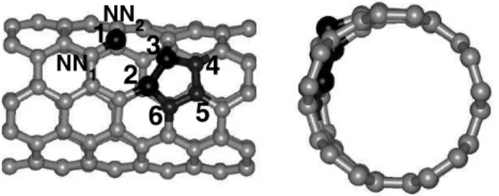
FIG. 4: Two different views of a detail of the (5,5) nanotube with a single vacancy, lateral (left) and frontal (right). The nearest-neighbor atoms to the vacancy are marked from 1 to 3, and are represented by larger spheres, and the atoms that reconstruct forming a pentagon are marked from 2 to 6. The relevant interatomic distances are given in Table I.
We begin by studying the single vacancy using a regu-lar supercell approximation. The calculations are simiregu-lar to what we have performed before for doped single wall car-bon nanotubes (SWNT) [29–33]. They are all based on first-principles density-functional theory calculations using the SIESTA code[7], which performs a fully self-consistent calculation solving the standard Kohn-Sham equations using a numerical, strictly localized basis set to expand the Kohn-Sham orbitals. For the exchange and correlation energy and potential we use the PBE-GGA [34]. In the geometry relax-ation calculrelax-ations we have used a split-valence double-zeta
TABLE I: Interatomic distances ( ˚A) between the marked atoms in Fig. 4. As a reference, the distance between two carbon atoms in a pristine (5,5) SWNT is also shown ((CC)bulk). The number in
paren-thesis for the 2-3 distance is the distance between these atoms in a pristine nanotube,i.e., before relaxation.
NN1-1 NN2-1 2-3 3-4 4-5 5-6 6-2 (C-C)bulk
1.42 1.42 1.59 (2.47) 1.48 1.43 1.44 1.44 1.45
basis set with a confining energy shift of 0.1 eV[35]. Stan-dard norm-conserving Troullier-Martins pseudopotentials[36] are used. A cutoff of 250 Ry for the grid integration was used to represent the charge density. We only considered a (5,5) SWNT (diameter of 6.92 ˚A). Our supercell has a lat-eral separation of 19 ˚A between image tube centers to make sure that they do not interact with each other. The supercell used in the geometry relaxations had 220-1=219 atoms (11 unit cells), which resulted in the value of 27.445 ˚A for the distance between a vacancy and its image in the next super-cell. This is the structure shown in Fig. 3. We have used 5 Monkhorst-Packk-points for the Brillouin zone integration along the tube axis, and the structural optimizations were per-formed using the conjugate gradient algorithm until the resid-ual forces were smaller than 0.05 eV/ ˚A. The atoms shown in lighter gray in Fig. 3 were held fixed at their bulk positions throughout the calculations. They will be the PL atoms within the central region.
A detail of the final geometry is shown in Fig. 4, both from a lateral as well as from a front view. The three atoms that are nearest-neighbors to the vacancy are shown as larger spheres, and are marked from 1 through 3. Atom 1 moves outward with respect to the original diameter, and atoms 2 and 3 get closer together and move inward. The distance between these atoms in a pristine (5,5) SWNT is 2.47 ˚A, since they are origi-nally second nearest neighbors. After the relaxation, this same distance becomes 1.59 ˚A, and there is the formation of a pen-tagon, as indicated in Fig. 4. This pentagon suffers an inward relaxation, as can be seen in Fig. 3. This flexibility of SWNT that allows these inward relaxations with relatively low energy cost has as a consequence that defects can have a much lower formation energy as compared to graphene sheets[37]. All the other relevant distances are presented in Table I.
We now turn to the charge transport calculations. All the details of the calculation, such as basis set, energy shift and real space grid, are the same as in the geometry relaxation calculations. In fact, the size of the supercell was suggested by the requirements of the transport calculations, since due to the localization range of the used basis set, the PL region needs to have three bulk unit cells[38]. Therefore, the central region contains two PL regions, one to the left and one to the right side of the extended molecule, which has 5 bulk unit cells (this is the region where the vacancy is located). For the leads (bulk) calculations we thus have to also use a supercell with three bulk unit cells, since this is exactly one PL region.
FIG. 5: Comparison between the transmittance and the band struc-ture for the geometry used as leads in the transport calculation.
the transmittance at a certain energy is equal to the number of right (or left) propagating Bloch states with the same energy. These are equivalent to “positive” (or “negative”)kz, wherek
is the wave vector characterizing a Bloch state in the Brillouin zone (BZ) of this periodic system, andzis thetransport direc-tion. Thus, the transmittance in this case could also be directly extracted from the band structure, whereT(E)is equal to the number of bands that are crossed at this energy, increasingkz
from either theΓpoint to BZ boundary (right propagating) or from the BZ boundary to theΓpoint (left propagating)[39]. With this procedure, we can check that the surface Green’s function is properly calculated, and know the upper bound for the transmittance obtained in the scattering calculation, spe-cially at the Fermi energy.
Using the relaxed geometry described above, that already includes the electrode regions of the left and right leads that are needed, we did a scattering region calculation, and ob-tained the transmittance shown in Fig. 6. As can be seen, the agreement with TranSIESTA is very good.
FIG. 6: Transmittance of a single vacancy in a (5,5) carbon nanotube. We show results obtained with TranSIESTA[5] and TRANSAMPA.
We can see that our calculation predicts a reduction of the
transmittance at the Fermi level by∼25%, when a single va-cancy is present (T(EF)drops from 2 G0toT(EF)∼1.5 G0, with G0=2e2/h). The important feature in the present calcu-lation is not the particular value ofT(EF), which may change
with the use of a larger basis set, but the almost perfect agree-ment between TRANSAMPA and TranSIESTA.
IV. CONCLUSION
In summary, we presented the details of a numerical imple-mentation of the DFT-NEGF method for charge transport cal-culations, which we have called TRANSAMPA. The DFT part of the method is based on the SIESTA code, and all the flex-ibilities of this program can be used in TRANSAMPA, such as multiple-ζbasis functions and spin polarized calculations. We illustrated the use of TRANSAMPA with the calculation of the transmittance of a single vacancy in a (5,5) SWNT. We compared our results with the TransSiesta code, and the agree-ment is excellent. Even though we only show results for a carbon nanotube, the method is very flexible, and can be used for a variety of situations of charge transport across nanos-tructures, such as, for example, molecules connecting two Au leads [40], or metallic nanowires with or without impurities. Of course the DFT-NEGF as implemented here is not the final answer to the challenging problem of quantitatively predict-ing the charge transport properties across nanosystems. How-ever, it is an important first step that will allow us to learn a great deal about those physical problems, even though in some cases we can only learn why it does not work.
V. ACKNOWLEDGEMENTS
We would like to thank Prof. E. Z. da Silva and Prof. S. R. A. Salinas for many helpful discussions.
We acknowledge support from FAPESP and CNPq, and CENAPAD-SP for computer time.
APPENDIX A: TIME REVERSAL SYMMETRY
If the system has time reversal symmetry, we have
ˆ
T−1HˆTˆ =Hˆ (A1)
where ˆT is the (antilinear) time reversal operator [41]. The operator definition of the Green’s function,
¡
E+ˆ1−Hˆ¢Gˆr(E) =ˆ1, (A2)
¡
E+ˆ1−Tˆ−1HˆTˆ¢Gˆr(E) =ˆ1, ¡
E−Tˆ−HˆTˆ¢Gˆr(E) =Tˆ, ¡
E−ˆ1−Hˆ¢ˆ
TGˆr(E)Tˆ−1=ˆ1, ¡ˆ
Ga(E)¢−1ˆ
TGˆr(E)Tˆ−1=ˆ1,
(A3)
so that
ˆ
TGˆr(E)Tˆ−1=¡ˆ
Gr(E)¢†
. (A4)
Given an operator ˆQ[41] such that
ˆ
TQˆTˆ−1=
( ˆ
Q, Qˆreal.
−Qˆ, Qˆcomplex, (A5)
we can decompose ˆGr(E)into its real and imaginary parts, ˆ
TGˆr(E)Tˆ−1=¡ˆ
Gr(E)¢∗
=¡ˆ
Gr(E)¢†
. (A6)
[1] See articles and references inIntroducing Molecular Electron-ics (Lecture Notes in PhysElectron-ics), Eds. G. Cuniberti, G. Fagas, and K. Richter, Springer-Verlag, Berlin, 2005.
[2] S. Datta. Electronic Transport in Mesoscopic Systems. Cam-bridge University Press, CamCam-bridge, 2001.
[3] J. Taylor, H. Guo, J. Wang, Phys. Rev B63, 245407(2001) [4] Y. Xue, S. Datta, and M. A. Ratner, Chem. Phys. 281,
151(2002).
[5] M. Brandbyge, Jos-Luis Mozos, P. Ordejn, J. Taylor, and K. Stokbro, Phys. Rev. B65, 165401 (2002).
[6] P. Hohenberg and W. Kohn, Phys. Rev136, 864B (1964); W. Kohn and L. J. Sham, Phys. Rev.140, 1133A (1965); W. Kohn, Rev. Mod. Phys.71, 1253 (1999).
[7] J. M. Soler, E. Artacho, J. D. Gale, A. Garc´ıa, J. Junquera, P. Ordej´on, and D. S´anchez-Portal, J. Phys.-Cond. Matt.14, 2745 (2002).
[8] This acronym is related to two words, TRANsport and SAMPA, which is by itself an acronym from the portuguese: Simulac¸˜oesAplicadas aMateriais: PropriedadesAtom´ısticas. To obtain the code, please contact either [email protected] or [email protected].
[9] Y. Meir and N. S. Wingreen, Phys. Rev. Lett.68, 2512 (1992). [10] L. V. Keldysh, Sov. Phys. JETP 20, 1018 (1965); L. P.
Kadanoff and G. Baym,Quantum Statistical Mechanics, Ben-jamin, Menlo Park, 1962.
[11] R. Landauer, Philos. Mag.21, 863 (1970); M. B¨uttiker, Y. Imry, R. Landauer, and S. Pinhas, Phys. Rev. B31, 6207 (1985); M. B¨uttiker, Phys. Rev. Lett.57, 1761 (1986).
[12] A. R. Rocha, V. M. Garcia-Surez, S. W. Bailey, C. J. Lambert, J. Ferrer, and S. Sanvito, Phys. Rev. B73, 085414 (2006). [13] For a general discussion and references, see K. Capelle,
cond-mat/0211443.
[14] M. P. L. Sancho, J. M. L. Sancho, and J. Rubio, J. Phys F:Met. Phys.14, 1205 (1984).
[15] E. N. Economou. Green’s Functions in Quantum Physics. Springer-Verlag, Berlin, 1990
[16] A. R. Williams, Peter J. Feibelman, and N. D. Lang, Phys. Rev. B26, 5433 (1982).
[17] H. Haug, AP. Jauho.Quantum Kinetics in Transport and Optics of Semiconductors. Springer-Verlag, Berlin, 1996
[18] Mathias Wagner, Phys. Rev. B44, 6104 (1991)
[19] J. Rammer and H. Smith, Rev. Mod. Phys.58, 323 (1986) [20] Kristian S. Thygesen, Phys. Rev. B73, 35309 (2006)
[21] This is not a restriction, since theextended molecule(as dis-cussed further in the text) can always be made larger, including more layers of the bulk geometry, such that this condition is satisfied
[22] Since TranSIESTA is a commercial code, the results we present were obtained during its trial period.
[23] S. Iijima, Nature354, 56 (1991).
[24] S. Iijima e T. Ichihashi, Nature 363, 603 (1993).
[25] Bethune, D. S.; Klang, C. H.; de Vries, M. S.; Gorman, G.; Savoy, R.; Vazquez, J.; Beyers, R. Nature363, 605 (1993). [26] See, for example, Carbon Nanotubes: Synthesis, Structure,
Properties and Applications, Eds. M. S. Dresselhaus, G. Dres-selhaus, and P. Avouris, (Topics in Applied Physics Series, Springer, Heidelberg, 2001).
[27] C. G´omez-Navarro, P. J. de Pablo, J. G´omez-Herrero, B. Biel, F. J. Garcia-Vidal, A. Rubio, and F. Flores, Nature Mat.4, 534 (2005).
[28] H. J. Choi, J. Ihm, S. G. Louie, and M. L. Cohen, Phys. Rev. Lett.84, 2917 (2000).
[29] R. J. Baierle, S. B. Fagan, R. Mota, A. J. R. da Silva, and A. Fazzio Phys. Rev. B64, 085413 (2001).
[30] S. B. Fagan, A. J. R. da Silva, R. Mota, R. J. Baierle, and A. Fazzio Phys. Rev. B67, 033405 (2003).
[31] S. B. Fagan, R. Mota, A. J. R. da Silva, and A. Fazzio Phys. Rev. B67, 205414 (2003).
[32] S. B. Fagan, R. Mota, A. J. R. da Silva, and A. Fazzio J. Phys.: Condens. Matter.16, 3647 (2004).
[33] S. B. Fagan, R. Mota, A. J. R. da Silva, and A. Fazzio Nano Lett.4, 975 (2004).
[34] J. P. Perdew, K. Burke, and M. Ernzerhof, Phys. Rev. Lett.77, 3865 (1996).
[35] E. Artacho, D. S´anchez-Portal, P. Ordej´on, A. Garcia, and J. M. Soler, Phys. Status Solidi B215, 809 (1999).
[36] N. Troullier and J. L. Martins, Phys. Rev. B43, 1993 (1991). [37] A. J. R. da Silva, A. Fazzio and A. Antonelli, Nano Lett.5, 1045
(2005).
[38] The size of the PL is determined in the electrode calculation, where it is chosen in such a way that, due to the strictly local-ized nature of the basis functions, one PL interacts only with its nearest neighbors. This is checked using the fact that the SIESTA code is designed to work with sparse matrices, and therefore easily provides which matrix elements are not strictly zero, allowing us to know if the supercell is interacting only with its two neighboring images.
[39] K. S. Thygesen, M. V. Bollinger, and K. W. Jacobsen, Phys. Rev. B67, 115404 (2003).
[40] R. B. Pontes, F. D. Novaes, A. Fazzio, and A. J. R. da Silva, J. Am. Chem. Soc.128, 8996 (2006).