610 Brazilian Journal of Physics, vol. 36, no. 3A, September, 2006
Dense Packings
H. J. Herrmann, R. Mahmoodi Baram, and M. Wackenhut
Institute for Computer Applications 1, University of Stuttgart, Pfaffenwaldring 27, D-70569 Stuttgart [email protected], [email protected], [email protected]
Received on 4 August, 2005
Dense packings of granular systems are of fundamental importance in the manufacture of hard ceramics and ultra strong concrete. We generalize the reversible parking lot model to describe polydisperse dynamic packings. The key ingredient lies in the size distribution of grains. In the extreme case of perfect filling of spherical beads (density one), one has Apollonian tilings with a powerlaw distribution of sizes. We will present the recent discovery of 3D packings which also have the freedom to rotate (bearings) in three dimensions.
Keywords: Granular systems, Dense packings, Polydispersive dynamics packings
I. INTRODUCTION
The search for the perfect packing has a long history [1] and although much is known about monodisperse or bidisperse systems, the real challenge lies in polydispersity. Materials of very high resistance made of an originally granular mix-ture as it is the case for high performance concrete (HPC) [2] and for hard ceramics are manufactured by trying to reach the highest possible densities. From the fracture mechanics point of view, higher densities imply less and smaller micro-cracks and therefore higher resistance and reliability. This goal can be reached as shown clearly for the case of HPC by mixing grains of very different sizes (gravel, sand, ordinary cement, limestone filler, silica fume), where the size distribution of the mixture follows as closely as possible a powerlaw distribution. In fact it is known that configurations of density one are ob-tained for spherical particles in so-called Apollonian packings (albeit not yet physically realisable) and constitute the ideal-ized final goal of a completely space filling packing having absolutely no defects.
In the studies presented here, on the one hand we general-ize a toy model for granular compaction, namely the reversible parking lot model to size distributions following a powerlaw. On the other hand we will discuss possible different realisa-tions and self similar packings in three dimensions.
II. A REVERSIBLE PARKING LOT MODEL FOR POLYDISPERSE SIZE DISTRIBUTIONS
Parking lot models have served as simple representations of compaction phenomena. Ben-Naim and Krapivski [3] in-troduced a reversible parking lot model to describe the com-paction dynamics of monodisperse packings. They found an asymptotically logarithmic approach to a final density which was confirmed experimentally by Knight et al. [4]. The model is defined within a one-dimensional interval on which parti-cles of fixed size are randomly absorbed with a ratek+and desorbed with a ratek−
. The density reached after an infinite time depends on the ratiok−/k+and is unity when this ratio
vanishes.
For strongly polydisperse size distributions, this model must be considerably modified in order to still make sense [5].
• A finite reservoir of particles must be considered in or-der to keep the distributions the same and this reservoir must be essentially not larger than the actual particles one would need to fill the interval.
• The system must be initialized very carefully by putting first the large particles, otherwise small particles will create huge voids.
• A size dependent desorption probability must be con-sidered, otherwise the large particles will easily leave the system without being able to be reinserted.
Our model is defined in the following way: Letribe the di-ameter of the ith-particle. Then the reservoir is filled with K particles following a distribution proportional to r−b
i for ri ∈[rmin,rmax] and fulfilling the constraint∑Ki ri=l where lis the length of the interval. The system is initialized by in-serting the particles according to their size, starting with the largest one. Each particle getsIattempts to find a free space in the interval and when it does, it will be left there. IfIis large enough, most particles will actually already be placed in this initial state. Once this procedure is finished, i.e. all particles in the reservoir have had theirIattempts, the real compaction dynamics is switched on by choosing randomly one of the re-maining particles from the reservoir and attempting to absorb it and then choosing randomly a particle in the interval with probabilityp(r)in order to desorb it. Each such step is called a time unit and typically we performt=109such units. The desorption probability is defined through
p(r) =
K1
∑
i=1
′
(hi−r)/l (1)
whereK1is the number of particles on the interval,hithe size of the ith-hole and the prime at the sum denotes that the sum only goes over positive terms and the negative ones are dis-carded.
In Fig. 1 we see an example for the evolution of the density as function of time. The first part with the steepest increase corresponds to the initialization (up tot=107) and the density reached at this point is calledρinit. From there we continue
H. J. Herrmann et al. 611
0.55 0.6 0.65 0.7 0.75 0.8 0.85 0.9 0.95 1
1 10 100 1000 10000
ρinit
I (density as function of time)
rmin=0.001
FIG. 1: Density as function of time.
the same time scale untilt=109. The full line is a fit using
the equation
ρinit(I) =ρmax−
∆ρ
1+B·ln(1+I/τ)I
−fn (2)
while the dotted line is obtained when the quotient in Eq. (2) is removed,∆ρ,B,τandfnare essentially fit parameters. One sees that on a logarithmic time scale eventually densities close to unity can be obtained. A particularly interesting result of this model is presented in Fig. 2 where the finally reached density at fixedIis shown as a function of the exponent of the powerlaw size distribution. We see that there exists an opti-mal value forbaround 1.6. Generalising the above model to higher dimensions should therefore be a way to help design-ers of stronger materials optimizing the size distribution of the grain mixture.
0.944 0.946 0.948 0.95
1.3 1.35 1.4 1.45 1.5 1.55 1.6 1.65 1.7 1.75 1.8 1.85
ρinit
b I=100
FIG. 2: Density after the initialization as function of the exponentb of the size distribution.
III. SPACE FILLING PACKINGS
In this section, we show how the, so-called,inversion al-gorithm [7] can be used to construct four new packings of spheres, including a packing with the important property of having only two classes of spheres such that no spheres from the same class touch each other. We refer to this packing as thebichromaticpacking [8]. As we will see, for special con-figurations of angular velocities of the spheres, this packing acts like a three dimensional bearing.
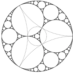
FIG. 3: Apollonian packing of circles. The dashed circles are the inversion circles.
A. Packings in two dimensions
Figure III B illustrates how the inversion algorithm can be employed to construct a simple packing of circles within an envelopping circle of unit radius. Initially three mutually touching circles are inscribed inside a circular space which is to be filled. Four inversion circles are set such that each of them is perpendicular to three of the four circles (three initial circles and an envelopping unit circle.)
Beginning with this configuration, if all pointsoutsidean inversion circle are mapped inside, one new circle is gener-ated, since the image of a circle perpendicular to the inversion circle falls on itself [10]. If the same is done for the other in-version circles, four new circles are generated inside the cor-responding inversion circle. In this way in the limit of infinite iterations we obtain the well-known Apollonian packing, in which the circular space is completely filled with circles of many sizes.
612 Brazilian Journal of Physics, vol. 36, no. 3A, September, 2006
B. Generalization to three dimensions
As a first guess for extending inversion algorthim to three dimension, one can set the initial spheres on vertices of a reg-ular polyhedron, namely, the fivePlatonic Solids, all inside a unit sphere. In this case, there will be one inversion sphere correspoding to each face of the Platonic Solid, perpendicular to the unit sphere plus the initial spheres forming that face. In addition, an inversion sphere is set in the center perpendicu-lar to all initial sphere. Using this configuration of initial and inversion spheres, the process of filling space is similar to in two dimensions, that is, iterative inversion of initial spheres and their images.
This algorithm was first used by Peikert et al [7] to re-produce the classic Apollonian, the only previously-known, packing of spheres, which is tetrahedron-based. Examining other Platonic Solids, we could produce four new packings; twobased on octahedron, one based on cube, one based on octahedron andnonebased on icosahedron.
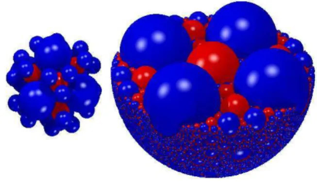
Figures??and 5 show two of obtained packings. The im-age on the left of each figure shows the packing afterone gen-eration and the one on the right shows the same packing in-cluding all spheres with radii larger than 2−7. The spheres are
grouped into different classes (assigned by different colours) such that no spheres having the same colour touch each other. Among the packings, there is one with only two colours (see Fig. 5.) We call this packing bichromatic. This has an immediate implication, that every loop of spheres in this pack-ing contains an even number of spheres. We now show that this is a sufficient condition for the spheres in contact to rotate without slip or even twist, which leads us to construction of the first space filling bearing in three dimension.
FIG. 4: The cube-based packing.
C. Space-filling bearings in three dimensions
In this section, we discuss the existence of a space filling bearing in three dimensions. We find out that the only
topo-FIG. 5: The bichromatic packing which is the second octahedron-based packing. No spheres of the same colour touch each other.
logical condition, under which the packing can work like a bearing, is that the packing be bichromatic, or equivalently, any loop of touching spheres consists of even number of spheres. Fulfilling this condition, one needs only to choose the right angular velocities for each sphere in order to no two spheres slip on each other, as will be discuss below.
First, we consider a single loop ofnspheres. The no-slip condition implies each pair of touching spheres have the same tangent velocities~vat their contact point. This condition for the contact between the first and the second sphere can be written as:
~v1=~v2
⇒ R1rˆ12×~ω1=−R2rˆ12×~ω2
⇒ (R1~ω1+R2~ω2)×rˆ12=0, (3)
whereR1,R2,~ω1and~ω2are the radii and the vectorial angular
velocities of the first and second sphere, respectively. ˆr12is the
unit vector in the direction connecting the centers of the first and the second sphere. From Eq.(3) the vector(R1~ω1+R2~ω2)
should be parallel to ˆr12:
R2~ω2=−R1~ω1−α12rˆ12, (4)
whereα12is an arbitrary parameter. Equation (4) is a
connec-tion between the rotaconnec-tion vectors~ω1and~ω2of the two spheres
in contact. Similarly for the third sphere in contact with the second, we have
R3~ω3=−R2~ω2−α23rˆ23. (5)
Putting Eq.(4) into Eq.(5) we find the relation between the angular velocities of the first and third sphere:
R3~ω3=R1~ω1+α12rˆ12−α23rˆ23. (6)
H. J. Herrmann et al. 613
by:
Rj~ωj= (−1)j −1R
1~ω1+
j−1
∑
i=1
(−1)j−iαi,i+1rˆi,i+1. (7)
As long as the chain is open, the spheres can rotate without slip with the angular velocities given by Eq.(7) and no restric-tions onαi,i+1. But, for a loop ofnspheres in contact, spheres
jandj+nare identical, so that
R1~ω1= (−1)nR1~ω1+
n
∑
i=1
(−1)n−i+1αi,i+1rˆi,i+1. (8)
A similar equation holds for every sphere j=1,· · ·,nin the loop.
Although for a single loop there are many solutions of Eq.(8), not all will serve our purpose. In a packing, each sphere belongs to a very large number of loops and all loops should be consistent and avoid frustration. In other words, the angular velocity obtained for a sphere as a member of one loop should be the same as being a member of any other loop. If the loop contains an even number n of spheres, Eq.(8) becomes a relation between the hitherto arbitrary coefficients of connectionαi,i+1,
n
∑
i=1
(−1)iαi,i+1rˆi,i+1=0. (9)
Using the fact that the loop is geometrically closed: n
∑
i=1
(Ri+Ri+1)rˆi,i+1=0, (10)
a solution for Eq.(9) is
αi,i+1=c(−1)i(Ri+Ri+1), (11)
wherecis an arbitrary constant. Putting this in Eq.(7), yields the angular velocities
~ωj= 1 Rj
(−1)j
³
−R1~ω1+c~R1j
´
, (12)
where~R1jis the vector which connects the centers of the first and jth sphere. As can be seen, the angular velocities only depend on the positions of the spheres, so that the consistency between different loops can be automatically fulfilled provid-ing that the parametercis the same for every loop of the entire packing.
In Eq.(12), all the angular velocities are calculated from~ω1
andc, which can be chosen arbitrarily. (c=0 corresponds to the case when all angular velocities are parallel.)
The no-slip condition (4) then reads
R1~ω1+R2~ω2=c~R12, (13)
so that the vectors~ω1,~ω2and~R12 are coplanar (the plane of
Fig.3, containing the two centers and the point of contactA). They are in general not collinear. Similarly, the angular veloc-ity of all spheres, under which the packing acts as a bearing, can be obtained.
IV. CONCLUSION
The highest possible densities are reached by polydis-perse granular packings. We have presented a simple one-dimensional model, showing that one can logarithmically slowly attain densities above 95 % and that one can optimize this number by tuning the exponent of the distribution. We have also seen that the idealized completely dense case can be self-similar in five topologically different configurations, only one of them having the property of being a bearing, i.e. allowing for slipless rotations around an arbitrary axis.
A full three-dimensional model or simulation of a system is still far from being realised because of the difficulties to deal with the large amount of very small particles. Our contribu-tions are just a small step in this direction. From the theo-retical point of view one has also to consider non-self-similar perfect packings and non spherical particles, understand the settling and demixing dynamics and calculate for each size the corresponding mobilities. From a numerical point of view, one has to organize the data hierarchically, eventually using quad-trees for a generalized linked cell algorithm and consider size classes in representative volume elements. We think that in the future much progress can still be achieved.
[1] T. Aste and D. Weaire, The pursuit of perfect packing. Institute of Physics Publishing, Bristol and Philadelphia 2000.
[2] F. de Larrard, Concrete Mixture Proportioning. Eds. E & FN Spon, London, New York 1999.
[3] E.R. Nowak, J.B. Knight, E. Ben-Naim, H.M. J¨ager, and S.R. Nagel, Physical Review E,57(2), 1982 (1998).
[4] J.B. Knight, C.G. Frandich, Chun Ning Lau, H.M. J¨ager, and S.R. Nagel, Physical Review E,51(1), 3957 (1995).
[5] M. Wackenhut and H.J. Herrmann, Searching for the perfect packing. Preprint, 2003.
[6] D.W. Boyd, Math. Comp.27(122), 369 (1973).
[7] M. Borkovec, W. de Paris, and R. Peikert, Fractals2(4), 521 (1994).
[8] R. Mahmoodi Baram, H.J. Herrmann, and N. Rivier, Phys. Rev. Lett.92, 044301 (2004).
[9] R. Mahmoodi Baram, H. J. Herrmann, Fractals12(3), 293 (2004).