doi: 10.1590/0101-7438.2016.036.02.0301
MONITORING THE STATOR CURRENT IN INDUCTION MACHINES FOR POSSIBLE FAULT DETECTION: A FUZZY/BAYESIAN APPROACH
FOR THE PROBLEM OF TIME SERIES MULTIPLE CHANGE POINT DETECTION
Marcos F.S.V. D’Angelo
1*, Reinaldo M. Palhares
2,
Renato D. Maia
1, Jo˜ao B. Mendes
1, Petr Ya. Ekel
3,
Camila K.S. Cangussu
1and Lucas A. Aguiar
1Received January 27, 2016 / Accepted May 18, 2016
ABSTRACT.This paper addresses the problem of fault detection in stator winding of induction machine by a multiple change points detection approach in time series. To handle this problem a new fuzzy/Bayesian approach is proposed which differs from previous approaches since it does not require prior information as: the number of change points or the characterization of the data probabilistic distribution. The approach has been applied in the monitoring the current of the stator winding induction machine. The good results obtained by proposed methodology illustrate its efficiency.
Keywords: Fuzzy/Bayesian, multiple change points detection, fault monitoring.
1 INTRODUCTION
Fault detection and analysis is a very important strategy that is commonly employed in the in-dustry with the purpose of allowing a cost-effective maintenance policy, keeping productivity standards and ensuring safety. The fault analysis gives support for the design of corrective ac-tions, system redundancies, and safety policies in order to mitigate the effects of a fault [33]. A fault diagnosis procedure is typically divided into three tasks:
i) fault detection, indicating the occurrence of some fault in a monitored system;
*Corresponding author.
1Universidade Estadual de Montes Claros – UNIMONTES, Departamento de Ciˆencia da Computac¸˜ao, Av. Rui Braga, s/n, 39401-089 Montes Claros, MG, Brasil. E-mails: [email protected]; [email protected]; [email protected]; [email protected]; [email protected]
2Universidade Federal de Minas Gerais, Departamento de Engenharia Eletrˆonica, Av. Antˆonio Carlos, 6627, Pampulha, 31270-901 Belo Horizonte, MG, Brasil. E-mail: [email protected]
ii) fault isolation, establishing the type and/or location of the fault; and
iii) fault identification, determining the magnitude of the fault.
After a fault has been detected and diagnosed, in some applications it is required that the fault be self-corrected, usually through controller reconfiguration. This is usually referred to as fault accommodation.
The literature presents several classes of strategies to deal with fault detection and isolation (FDI) [14]. These strategies can be, in general, divided in approaches based on quantitative models [68] and on qualitative models [66], [67].
Most of the quantitative model-based approaches are based on the knowledge of mathematical models of the plant. Many survey papers with different emphasis on various model-based ap-proaches have been published over the past years. The main apap-proaches in this context are based on (unknown input) observers [14], [15], [16], [52], [62], [63], parity relations [14], [50] and Kalman or robust filters [1], [14], [28], [29], [72]. The requirement of a mathematical model of the plant can lead to several difficulties in the implementation of these approaches, for instance due to factors such as system complexity, high dimensionality, nonlinearities and parametric uncertainties.
On the other hand, most of the qualitative model approaches are based on some pattern analysis of the historical process data. The main related approaches are: signed directed graph [5], [13], [47], fault tree [23], fuzzy systems [18], [25], [54], qualitative trend analysis [20], [22], [26], [48], mutual information [69], neural networks [12], [17] (neural networks also can be used as observer [64], [51]), artificial immune systems [43], [44], [57], Bayesian networks [65], [70] and the combination of techniques [19], [38].
In this paper, a new quantitative approach for fault monitoring is presented. This new approach is based on a fuzzy/Bayesian representation and was extended to the detection of multiple change points, not just one or two change points as in [20] and [46], respectively. To illustrate the effi-ciency of the proposed methodology, the problem of monitoring the stator current of induction machine, for possible fault detection, has been solved.
Induction motors are the most important electric machinery for different industrial applications. Faults in the stator windings of three-phase induction motor represent a significant part of the failures that arise during the motor lifetime. When these motors are fed through an inverter, the situation tends to become even worse due to the voltage stresses imposed by the fast switching of the inverter [11]. From a number of surveys, it can be realized that, for the induction motors, stator winding failures account for approximately 30% of all failures [2], [34].
Although there is no experimental data that indicate the time delay between inter-turn and ground insulation failure, it is believed that the transition between the two states is not instantaneous. Therefore, early detection of inter turn short circuit during motor operation can be of great sig-nificance as it would eliminate subsequent damage to adjacent coils and the stator core, reducing repairing cost and motor outage time [6], [59].
However, early stages of deterioration are difficult to detect. In general, most of the previous references present approaches for dealing with abrupt faults in the stator winding, which are eas-ier to be detected than incipient faults. In spite of these difficulties, a great deal of progress has been made on induction machine stator-winding incipient fault detection. Methods that use volt-age and current measurements offer several advantvolt-ages over test procedures that require machine to be taken off line or techniques that require special sensors to be mounted on the motor [58]. Other methods, in the context of fault related to the stator-winding, can be found in [9], [10], [24], [53], [61]. There exist other type of approaches to deal with different faults in induction machine, unlike the one considered in this paper, as, for example, dynamic eccentricity, unbalanced rotors, bearing defects and broken rotor bars (see [56] for details and further references).
This paper is organized as follows. Section 2 shows the new fuzzy/Bayesian approach. Section 3 presents and analyzes the induction machine modeling considering the case of turn-to-turn short circuit in stator winding and shows the results for monitoring stator current of induction machine. Finally, section 4 presents the concluding remarks.
2 FUZZY/BAYESIAN APPROACH FOR MULTIPLE CHANGE POINTS DETECTION
Traditional methods of building models for time series are based on statistical techniques, aiming to select models that satisfactorily explain its dynamic behavior. However, some questions can be raised:
• There is regime change in the series?
• Can a single model to portray this dynamic for the whole data set?
is evaluated in identifying changes, proposed by [39], in the rate of the Poisson distribution in sequentially observed data, and a comparison being done with the one proposed by [30]. How-ever, all these researches require some a priori knowledge of the statistical behavior of the time series, for example, what type of distribution represents better its dynamic behavior. In this work, an approach that is independent of such a priori knowledge about the time series will be used, considering the empirical demonstration presented in [20] that series, after being transformed using fuzzy operations, can be adequately approximated by series with beta distribution. Thus, the parametrization of the beta distribution is used to replace a priori knowledge about the time series. Moreover, the method was extended to the detection of multiple change points, not just one or two change points as in [20] and [46], respectively.
2.1 Time Series Transformation by Fuzzy Sets
The fuzzy set theory, proposed by [71], has received much attention recently, not only in the context of theoretical developments, but also in applications. One of its main applications is in clustering methods, whereas classical methods of grouping the data intok separate categories, and in many cases some elements may not belong to a specific category, belonging to two or more categories simultaneously. Using fuzzy clustering methods is a good way to solve this problem because, unlike the classical approach, an element can belong to more than one cat-egory simultaneously.
Below it’s proposed an alternative quantization of a time series, throughfuzzyclustering, for use in theMetropolis-Hastingsalgorithm.
Definition(Fuzzy Clustering): Let y(t)be a time series, and consider a positive integer k. Define the setC = {Ci | min{y(t)} ≤Ci ≤max{y(t)},i =1,2, . . . ,k}such that it solves the minimization problem:
min k
i=1
µi(t)∈Ci
µi(t)−Ci 2, (1)
soC= {Ci,i=1,2, . . . ,k}is the set of centers of the time seriesy(t). In (1),
µi(t)
⎡
⎣
k
j=1
y(t)−Ci2 y(t)−Cj2
⎤
⎦
−1
(2)
is the fuzzy membership degree ofy(t)for each centerCi.
For illustration purposes, in this paper, the time series (3) is used:
f(t)=
⎧ ⎪ ⎪ ⎪ ⎪ ⎨
⎪ ⎪ ⎪ ⎪ ⎩
p1+0.1∗ε(t)−0.1∗ε(t−1), ift ≤m1;
p2+0.1∗ε(t)−0.1∗ε(t−1), ifm1<t ≤m2; ..
.
pk+0.1∗ε(t)−0.1∗ε(t−1), ift >mk−1.
⎫ ⎪ ⎪ ⎪ ⎪ ⎬
⎪ ⎪ ⎪ ⎪ ⎭
(3)
being p1the first operation point, p2the second operation point, pk thek−t hoperation point, ε(t)a noise with distributionπ(.)in the instantt, andmi the change points.
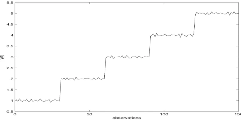
Figure 1 illustrates the time series (3) withp1=1, p2=2, p3=3, p4=4, p5=5,m1=30,
m2 = 60,m3 = 90,m4 = 120 andε(t) ∼ U(0,1)for 150 observations of the time series,
Figure 2 shows the centers of time series and the membership degreesµi(t)is illustrated by Figure 3. Note that the first and last membership degrees have a single change, which will be identified using the approach proposed by [20], and the intermediate membership degrees have two changes to be identified by the approach proposed by [46].
Figure 1–Time series with p1 =1, p2 =2, p3 =3, p4 =4, p5=5,m1=30,m2=60,m3=90,
m4=120 andε(t)∼U(0,1)for 150 observations.
The proposed fuzzy clustering to transform a given time series into a new one is described below:
1. Input the time series y(t);
2. Find the set ofk centers, C = {Ci | min{y(t)} ≤ Ci ≤ max{y(t)},i = 1,2, . . . ,k}, that minimizes the Euclidean distance as (1), considering, for example, the time series (3) (Fig. 1).
Figure 2–Centers of time series of Figure 1.
2.2 Formulation of the Metropolis-Hastings algorithm
The goal of the Metropolis-Hastings algorithm [27] is to construct a Markov chain that has a certain equilibrium distributionπ. Define a Markov chain as follows. If Xi−1 = xi−1, then
generate a candidate value X∗ from a distribution with density fX∗|X(y) = 1(xi−1,x∗). The functionq(.) is known as the core transition of the Markov chain. The candidate value X∗ is accepted or rejected with a probability of acceptance:
α(x,y)=min
1, π(x
∗)
π(xi−1)
q(x∗,xi−1)
q(xi−1,x∗)
(4)
If the candidate is accepted, do xi = Y, otherwise do xi = Xi−1. Thus, if the candidate
is rejected, the Markov chain repeats the sequence. It is possible to show that, under general conditions, the sequence X0,X1,X2, . . .is a Markov chain with equilibrium distributionπ. In
practical terms, the Metropolis- Hastings algorithm can be specified by the following steps:
1. Choose an initial valuex0, the number of simulations,R, and make the simulations counter
r=1;
2. Generate a candidate valuey∼q(xi, .);
3. Calculate the probability of acceptance as in (4) and generateu∼U(0,1);
4. Calculate the new value of the current state:
xt+1=
y, ifα(x,y) >u xt, otherwise
5. Ifr <R, return to step 2. Otherwise, stop.
Note that, as discussed in [21], the quantization technique generates a time series transformed to the first and last membership degree with the following probability distribution:
µi(t)∼Bet a(a,b), fort=1, . . . ,m µi(t)∼Bet a(c,d), fort=m+1, . . . ,n
The parameters to be estimated by Metropolis-Hastings algorithm area,b,c,d and the change pointm. In this type of algorithm, usually, uninformative priors are used, for example:
a∼Gamma(0.1,0.1)
b∼Gamma(0.1,0.1)
c∼Gamma(0.1,0.1)
d ∼Gamma(0.1,0.1)
m∼U[1, . . . ,n],withp(m)= 1
TheGammadistribution with parameters shape and scale equal to 0.1 was chosen because it is uninformative, with the goal of sweeping the entire parameter space. Considering the intermedi-ate membership degree, we have the following probability distribution:
µi(t)∼Bet a(a,b), fort =1, . . . ,mi−1 µi(t)∼Bet a(c,d), fort =mi−1+1, . . . ,mi µi(t)∼Bet a(e, f), tomi =t+1, . . . ,n
The parameters to be estimated by Metropolis- Hastings algorithm area,b,c,d,e, f and the second point of change,mi, whereas the first switch point,mi−1is identified in the previous step.
In this type of algorithm uninformative priors are commonly used, for example:
a∼Gamma(0.1,0.1)
b∼Gamma(0.1,0.1)
c∼Gamma(0.1,0.1)
d ∼Gamma(0.1,0.1)
e∼gamma(0.1,0.1)
f ∼Gamma(0.1,0.1)
mi ∼U[mi−1, . . . ,n],withp(m)=
1 n−mi
The transition kernels of the Markov chain for the model with a single point of change and for the model with two change points are presented in appendices A and B, respectively.
2.3 Example of multiple change point detection in time series presented in Figure 1
The proposed fuzzy/Bayesian multiple change points detection in time series is described below:
1. Input the time seriesy(t)(Fig. 1);
2. Find the set ofkcenters,C = {Ci |min{y(t)} ≤Ci ≤max{y(t)},i =1,2, . . . ,k}, given by Figure 2.
3. Compute thefuzzymembership degree given in (2), for each sample of the time series, y(t), with respect to each centerCi, illustrated by Figure 3.
4. Compute Metropolis-Hastings Algorithm in each membership function for change point detection as illustrated in Figure 4 (for first and last membership function is executed the detection of the one change point, and in the others membership functions is executed the detection of the two change points). The final analysis is performed as: the change point, mi, is obtained by checking where the maximum ofmi histogram occurs.
3 CASE STUDY: MONITORING INDUCTION MACHINE WITH TURN-TO-TURN
SHORT CIRCUIT IN STATOR WINDING
Figure 4–Results of proposed methodology.
due to many factors, which include thermal overload, mechanical vibration and peak voltage caused by a speed controller. The deterioration of insulation usually begins as a short circuit fault of the stator-winding. This section describes the model that is employed here for the simulation of inter-turn short circuits in the stator windings of induction machines.
This work employs a generic model for the machine [8], valid for anydq(direct and quadrature) axis speed obtained by the Park’s transformation [37]. Representing the currents, voltages and electromagnetic flows byi,vandλ, the resistance, leakage and mutual inductance byr,Ll and Lm, the phasesa,bandcby indexesa,bandc, the windings of the stator and rotor by indexes sandr, the stator and rotor voltages equations become:
[vs] = [rs][is] + d[λs]
dt (5)
[vr] = [rr][ir] + d[λr]
dt (6)
where
[vs] = [ vas1 vas2 vbs vcs ]T
[vr] = [ var vbr vcr ]T
[is] = [ ias ias−if ibs ics ]T
[λs] = [ λas1 λas2 λbs λcs ]T
[λr] = [ λar λbr λcr ]T
In the above, the indexas2represents the shorted turns andif is the current in the shorted turns. Figure 5 represents the schematic diagram of a motor with an inter-turn short circuit.
Figure 5–Representation of stator windings of a motor with inter-turn short circuit.
In the model proposed in reference [8], the stator windings voltages are given by:
Vds+ 2
3µrsifcosθ=rsids+ dλds
dt +ωλqs (7)
Vqs+ 2
3µrsif sinθ =rsiqs + dλqs
dt +ωλds (8)
V0s+ 1
3µrsif =rsi0s+ dλ0s
dt (9)
The rotor circuit equations are the same as for traditional symmetrical model.
The stator and the rotor electromagnetic flows of stator indqaxis, are given by:
λds=Lsids+Lmidr− 2
3µLsifcosθ (10)
λqs =Lsiqs+Lmiqr − 2
3µLsif sinθ (11)
λ0s =Llsi0s + µ
3Llsif sinθ (12)
λdr =Lridr +Lmids− 2
3µLmif cosθ (13)
λqr =Lriqr +Lmiqs− 2
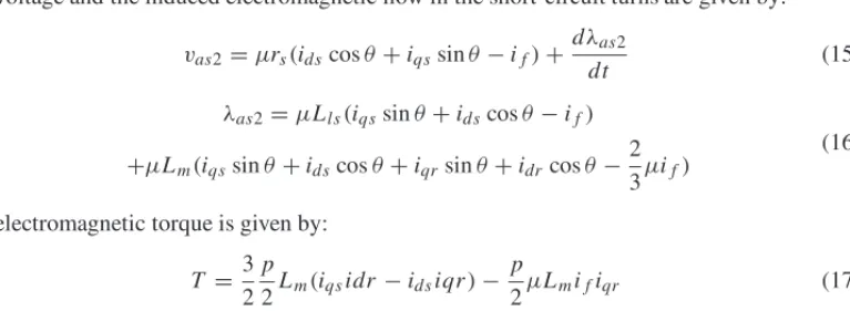
The voltage and the induced electromagnetic flow in the short-circuit turns are given by:
vas2=µrs(idscosθ+iqssinθ−if)+ dλas2
dt (15)
λas2=µLls(iqssinθ+idscosθ−if)
+µLm(iqssinθ+idscosθ+iqrsinθ+idrcosθ− 2 3µif)
(16)
The electromagnetic torque is given by:
T =3
2 p
2Lm(iqsidr −idsiqr)− p
2µLmifiqr (17)
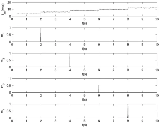
The induction machine stator current simulation results for a fault beginning which 2% of turns in the phaseabecome in short circuit after the time 2sand increase of 2% every time of 2sto reach a level of 8% of short-circuit is shown in the Figure 6. The root mean square (rms) current values is illustrated in Figure 7. The proposed monitoring for future fault detection approach here is based on finding such events of non-balanced changes in the currentrmsvalues.
Figure 6–Current of phasea.
3.1 Results of Proposed Methodology
Figure 7–rms current of phasea.
described in this Section and the change point detection methodology presented in Section 2. The centers in the induction machine currents are found by optimization of the Average Silhouette Width [55].
4 CONCLUSIONS
Figure 8–rms current of phaseaand the results of proposed methodology.
ACKNOWLEDGEMENTS
This work has been supported in part by the Brazilian agencies CNPq and FAPEMIG.
REFERENCES
[1] ALAVISMM, IZADI-ZAMANABADIR & HAYESMJ. 2008. Robust fault detection and isolation technique for single-input/single-output closed-loop control systems that exhibit actuator and sensor faults.IET Control Theoty and Applications,2(11): 951–965.
[2] ARKANM, PEROVICDK & UNSWORTHP. 2001. Online stator fault diagnosis in induction motors.
IEE Proceedings Electronic Power Application,148(6): 537–547, November.
[3] BEZDEKJC. 1981.Pattern recognition with fuzzy objective function algorithms. Plenum Press. [4] BARRYD & HARTIGANJA. 1993. A Bayesian analysis for change point problems.Journal of the
American Statistical Association,88(421): 309–319.
[5] BOUKHOBZAT, HAMELINF & CANITROTS. 2008. A graph-theoretic approach to fault detection and isolation for structured bilinear systems.International Journal of Control,81(4): 661–678. [6] BOQIANGX, HEMINGL & SUNLILING. 2003. Apparent impedance angle based detection of stator
winding interturn short circuit fault in induction motors. InProceedings of the Industry Application Conference, pages 1118–1125.
[8] BACCARINILMR, MENEZESBR & CAMINHASWM. 2010. Fault induction dynamic model, suit-able for computer simulation: simulation results and experimental validation.Mechanical Systems and Signal Processing,24: 300–311.
[9] BACCARINILMR, MENEZESBR, GUIMARAES˜ HN & CAMINHASWM. 2006. A method for early detection of stator winding faults. InProceedings of VII International Conference on Industrial Ap-plications, pages 1–6, Recife/Brazil.
[10] BALLALMS, SURYAWANSHIHM & MISHRAMK. 2008. Detection of incipient faults in induction motors using FIS, ANN and ANFIS techniques.Journal of Power Electronics,8(2): 181–191. [11] CRUZSMA & CARDOSOJM. 2004. Diagnosis of stator interturn short circuits in dtc induction
motor drives.IEEE Transactions on Industry Applications, 40(5): 1349–1360.
[12] CALADOJMF, KORBICZJ, PATANK, PATTON RJ &DACOSTAJMGS. 2001. Soft computing approaches to fault diagnosis for dynamic systems.European Journal of Control,7(2-3): 248–286. [13] CHENG H, NIKUSM & JAMSA-JOUNELA S. 2008. Fault diagnosis of the paper machine short
circulation process using novel dynamic causal digraph reasoning.Journal of Process Control,18(7– 8): 676–691.
[14] CHENJ & PATTONRJ. 1999.Robust model-based fault diagnosis for dynamic systems. Dordrecht: Kluwer Academic Publishers.
[15] CHENW & SAIFM. 2007. Observer-based strategies for actuator fault detection, isolation and esti-mation for certain class of uncertain nonlinear systems.IET Control Theoty and Applications,1(6): 1672–1680.
[16] CAMINHASWM & TAKAHASHIRHC. 2001. Dynamic system failure detection and diagnosis em-ploying sliding mode observers and fuzzy neural networks. InProceedings of the Joint 9th IFSA and 20th NAFIPS, pages 304–309, Vancouver.
[17] D’ANGELOMFSV & COSTAPP. 2001. Detection of shorted turns in the field winding of turbo-generators using the neural network mlp. InProceedings of the IEEE International Conference on Systems, Man, and Cybernetics, pages 1930–1935, Tucson.
[18] DETROJAKP, GUDIRD & PATWARDHANSC. 2006. A possibilistic clustering approach to novel fault detection and isolation.Journal of Process Control,16(10): 1055–1073.
[19] D’ANGELOMFSV, PALHARESRM, COSMELB, AGUIARLA, FONSECAFS & CAMINHASWM. 2014. Fault detection in dynamic systems by a fuzzy/bayesian network formulation.Applied Soft Computing,21: 647–653.
[20] D’ANGELO MFSV, PALHARES RM, TAKAHASHI RHC, LOSCHI RH, BACCARINI LMR & CAMINHASWM. 2011. Incipient fault detection in induction machine stator-winding using a fuzzy-Bayesian change point detection approach.Applied Soft Computing,11(1): 179–192.
[21] D’ANGELOMFSV, PALHARESRM, TAKAHASHIRHC & LOSCHIRH. 2011. A fuzzy/bayesian approach for the time series change point detection problem.Pesquisa Operacional,31: 217–234. [22] D’ANGELO MFSV, PALHARESRM, TAKAHASHIRHC & LOSCHIRH. 2011. Fuzzy/Bayesian
change point detection approach to incipient fault detection.IET Control Theory & Applications, 5(4): 539–551.
[24] DA SILVA AM, POVINELLIRJ & DEMERDASHNAO. 2008. Induction machine broken bar and stator short-circuit fault diagnostics based on three-phase stator current envelopes.IEEE Transactions on Industrial Electronics,55(3): 1310–1318.
[25] EL-SHALSM & MORRISAS. 2000. A fuzzy expert system for fault detection in statistical process control of industrial processes.IEEE Transactions on Systems, Man and Cybernetics, Part C,30(2): 281–289.
[26] FONGKF, LOHAP & TANWW. 2008. A frequency domain approach for fault detection. Interna-tional Journal of Control,81(2): 264–276.
[27] GAMERMAND. 1997.Markov chain Monte Carlo: stochastic simulation for Bayesian inference. Chapman & Hall.
[28] GAOH, CHENT & WANGL. 2008. Robust fault detection with missing measurements.International Journal of Control,81(5): 804–819.
[29] GAO Z, WANGH & CHAI T. 2007. A robust fault detection filtering for stochastic distribution systems via descriptor estimator and parametric gain design.IET Control Theoty and Applications, 1(5): 1286–1293.
[30] HARTIGAN JA. 1990. Partition models.Communication in Statistics-Theory and Methods,19(8): 2745–2756.
[31] HINKEYDV. 1971. Inference about the change point from cumulative sum test.Biometria,26: 279– 284.
[32] HADJILIADISO & MOUSTAKIDESV. 2006. Optimal and asymptotically optimal cusum rules for change point detection in the brownian motion model with multiple alternatives.Theory of Probability and its Applications,50(1): 75–85.
[33] ISERMANNR & BALLEP. 1997. Trends in the application of model-based fault detection and diag-nosis of technical processes.Control Engineering Practice,5(5): 707–719.
[34] IRAVANIMR & KARIMI-GHARTEMANIM. 2003. Online estimation of steady state and instan-taneous symmetrical components. IEE Proceedings Generation, Transmission and Distribution, 150(5): 616–622, September.
[35] KOHONENT. 2001.Self-organizing maps. Springer Series in Information Sciences. Springer. [36] KAUFMANL & ROUSSEEUWPJ. 1990.Finding groups in data: An introduction to cluster analysis.
John Wiley & Sons.
[37] KRAUSEPC. 1986.Analysis of Electric Machinery. McGraw-Hill.
[38] LAURENTYSCA, BOMFIMCHM, MENEZES BR & CAMINHASWM. 2011. Design of a pipeline leakage detection using expert system: A novel approach.Applied Soft Computing,11(1): 1057– 1066.
[39] LOSCHIRH & CRUZFRB. 2005. Bayesian identification of multiple change points in poisson data.
Advances in Complex Systems,8: 465–482.
[41] LOSCHIRH, GONC¸ALVESFB & CRUZFRB. 2005. Avaliac¸˜ao de uma medida de evidˆencia de um ponto de mudanc¸a e sua utilizac¸˜ao na identificac¸˜ao de mudanc¸as na taxa de criminalidade em belo horizonte.Pesquisa Operacional,25(3): 459–463.
[42] LEES, NISHIYAMAY & YOSHIDAN. 2006. Test for parameter change in diffusion processes by cusum statistics based on one-step estimators.Annals of the Institute of Statistical Mathematics,58(2): 211–222.
[43] LAURENTYSCA, PALHARESRM & CAMINHASWM. 2010. Design of an artificial immune system based on danger model for fault detection.Expert Systems with Applications,37(7): 5145–5152. [44] LAURENTYSCA, PALHARESRM & CAMINHASWM. 2011. A novel artificial immune system for
fault behavior detection.Expert Systems with Applications,38(11): 6957–6966.
[45] LEES, PARKS, MAEKAWA K & KAWAI K. 2006. Test for parameter change in arima models.
Communications in Statistics: Simulation and Computation,35(2): 429–439.
[46] MOREIRAFS, D’ANGELOMFSV, PALHARESRM & CAMINHASWM. 2010. Incipient fault de-tection in induction machine stator-winding using a fuzzy-Bayesian two change points dede-tection ap-proach. In9th IEEE/IAS International Conference on Industry Applications.
[47] MAURYAMR, RENGASWAMYR & VENKATASUBRAMANIANV. 2006. A signed directed graph-based systematic framework for steady-state malfunction diagnosis inside control loops.Chemical Engineering Science,61(6): 1790–1810.
[48] MAURYAMR, RENGASWAMYR & VENKATASUBRAMANIANV. 2007. Fault diagnosis using dy-namic trend analysis: A review and recent developments.Engineering Applications of Artificial Intelligence,20(2): 133–146.
[49] OH KJ, ROH TH & MOON MS. 2005. Developing time-based clustering neural networks to use change-point detection: Application to financial time series.Asia-Pacific Journal of Operational Research,22(1): 51–70.
[50] PLOIX S & ADROTO. 2006. Parity relations for linear uncertain dynamic systems.Automatica, 42(9): 1553–1562.
[51] PATANK & PARISINIT. 2005. Identification of neural dynamic models for fault detection and isola-tion: the case of a real sugar evaporation process.Journal of Process Control,15(1): 67–79. [52] PUIGV, STANCUA, ESCOBETT, NEJJARIF, QUEVEDOJ & PATTONRJ. 2006. Passive robust
fault detection using interval observers: Application to the DAMADICS benchmark problem.Control Engineering Practice,14(6): 621–633.
[53] RODRIGUEZPVJ & ARKKIOA. 2008. Detection of stator winding fault in induction motor using fuzzy logic.Applied Soft Computing,8: 1112–1120.
[54] RAGOTJ & MAQUIND. 2006. Fault measurement detection in an urban water supply network.
Journal of Process Control,16(9): 887–902.
[55] ROUSSEOUWPJ. 1987. Silhouettes: a Graphical Aid to the interpretation and Validation of Cluster Analysis.Computacion and Applied Mathematics,20: 53–65.
[57] SILVAGC, PALHARESRM & CAMINHASWM. 2012. Immune inspired fault detection and diagno-sis: A fuzzy-based approach of the negative selection algorithm and participatory clustering.Expert Systems with Applications,39(16): 12474–12486.
[58] SOTTILEJ, TRUTTFC & KOHLERJL. 2000. Experimental investigation of on-line methods for incipient fault detection in induction motors. InProceedings of the Industry Application Conference, pages 2682–2687.
[59] THOMSONWT & FENGERM. 2001. Current signature analysis to detect induction motor faults.
IEEE Industry Applications Magazine,7: 26–34, July/August.
[60] TALLAMRM, LEESB, STONEG, KLIMANGB, YOOJ, HABETLERTJ & HARLEYRG. 2003. A survey of methods for detection of stator faults in induction machines. InProceedings of SDEMPED, Diagnostics for Electric Machines, Power Eletronics and Drives, pages 35–46.
[61] TALLAMRM, LEESB, STONEGC, KLIMANGB, YOOJ, HABETLERTG & HARLEYRG. 2007. A survey of methods for detection of stator-related faults in induction machines.IEEE Transactions on Industry Applications,43(4): 920–933.
[62] TAKAHASHIRHC & PERESPLD. 1999. Unknown input observers for uncertain systems: A unify-ing approach.European Journal of Control,5(2–4): 261–275.
[63] TAKAHASHI RHC, PALHARES RM & PERES PLD. 1999. Discrete-time singular observers:
H2/H∞optimality and unknown inputs.International Journal of Control,72(6): 481–492. [64] UPPALFJ, PATTONRJ & WITCZAKM. 2006. A neuro-fuzzy multiple-model observer approach to
robust fault diagnosis based on the DAMADICS benchmark problem.Control Engineering Practice, 14(6): 699–717.
[65] VERRONS, LIJ & TIPLICAT. 2010. Fault detection and isolation of faults in a multivariate process with Bayesian network.Journal of Process Control,20(8): 902–911.
[66] VENKATASUBRAMANIANV, RENGASWAMYR & KAVURISN. 2003. A review of process fault detection and diagnosis – part II: Qualitative models and search strategies.Computers and Chemical Engineering,27: 313–326.
[67] VENKATASUBRAMANIANV, RENGASWAMYR, KAVURISN & YINK. 2003. A review of process fault detection and diagnosis – part III: Process history based methods.Computers and Chemical Engineering,27: 327–346.
[68] VENKATASUBRAMANIANV, RENGASWAMYR, YINK & KAVURISN. 2003. A review of process fault detection and diagnosis – part I: Quantitative model-based methods.Computers and Chemical Engineering,27: 293–311.
[69] VERRON S, TIPLICA T & KOBI A. 2008. Fault detection and identification with a new feature selection based on mutual information.Journal of Process Control,18(5): 479–490.
[70] XUBG. 2012. Intelligent fault inference for rotating flexible rotors using Bayesian belief network.
Expert Systems with Applications,39(1): 816–822.
[71] ZADEHLA. 1965. Fuzzy sets.Information and Control,8(3): 338–353.
APPENDIX A
This appendix is intended to build the probabilities of acceptance for the posterior distribution of the parametersa,b,c,d and mdescribed in theMetropolis-Hastingsalgorithm. The reference distributions used in the work are the prior distributions, i.e., theGamma(0.1,0.1), that have been chosen to be uninformative.
1. For the parametera:
(a∗) (ai−1)
q(a∗,ai−1)
q(ai−1,a∗) =
Ŵ a∗+bi−1
Ŵ(a∗)
mi−1mi−1
j=1
yaj∗−1
ai−1 a∗
0.9
e−0.1
a∗−ai−12
Ŵ(ai−1+bi−1)
Ŵ(ai−1)
mi−1mi−1
j=1
yaji−1−1
2. For the parameterb:
(b∗) (bi−1)
q(b∗,bi−1)
q(bi−1,b∗) =
Ŵ ai+b∗
Ŵ(b∗)
mi−1mi−1
j=1
1−yj b∗−1
bi−1 b∗
0.9
e−0.1b∗−bi−1
2
Ŵ(ai−1+bi−1)
Ŵ(bi−1)
mi−1mi−1
j=1
1−yjb
i−1−1
3. For the parameterc:
(c∗) (ci−1)
q(c∗,ci−1)
q(ci−1,c∗) =
Ŵ c∗+di−1
Ŵ(c∗)
n−mi−1 n
j=mi−1+1 ycj∗−1
ci−1 c∗
0.9
e−0.1c∗−ci−1
2
Ŵ(ci−1+di−1)
Ŵ(ci−1)
n−mi−1 n
j=mi−1+1 ycji−1−1
4. For the parameterd:
(d∗)
(di−1)
q(d∗,di−1)
q(di−1,d∗) =
Ŵ ci+d∗
Ŵ(d∗)
n−mi−1 n
j=mi−1+1
1−yj
d∗−1
di−1 d∗
0.9
e−0.1d∗−di−1
2
Ŵ(ci−1+di−1)
Ŵ(di−1)
n−mi−1 n
j=mi−1+1
5. For the parameterm:
m∗ mi−1
q
m∗,m
q
mi−1,m∗ =
Ŵai+bi
Ŵ ai
Ŵ bi
m∗
Ŵci+di
Ŵ ci
Ŵ di
n−m∗ m∗
j=1
yaji−1 1−yjb
i−1 n
j=m∗+1
ycji−1 1−yjd
i−1
Ŵ ai+bi
Ŵ ai
Ŵ bi
mi−1
Ŵ ci+di
Ŵ ci
Ŵ di
n−mi−1mi−1
j=1
yaji−11−yjb
i−1 n
j=mi−1+1
ycji−11−yjd
i−1
APPENDIX B
This appendix is intended to show the probabilities of acceptance for the posterior distributions of the parametersa, b, c, d, e,f,m1 andm2 described in theMetropolis-Hastingsalgorithm
for the model with two changes and remembering that the pointm1will always be obtained by
the previous series, it is not necessary then that will be treasured. The reference distributions used here are his own prior distributions, which in this work distributionsGamma(0.1,0.1)were chosen to be uninformative.
1. For the parametera:
(a∗) (a)
q(a∗,a)
q(a,a∗) =
0.10.1[Ŵ (0.1)]−1a∗0.1−1e−0.1a∗2
0.10.1[Ŵ (0.1)]−1a0.1−1e−0.1a2
m1
i=1
Ŵ(a∗+b)
Ŵ(a∗)Ŵ(b)ya ∗−1 i
m1
i=1 Ŵ(a+b) Ŵ(a)Ŵ(b)y
a−1
i
2. For the parameterb:
(b∗) (b)
q(b∗,b)
q(b,b∗) =
0.10.1[Ŵ (0.1)]−1b∗0.1−1e−0.1b∗2
0.10.1[Ŵ (0.1)]−1b0.1−1e−0.1b2
m1
i=1
Ŵ(a+b∗)
Ŵ(a)Ŵ(b∗)yb ∗−1 i
m1
i=1 Ŵ(a+b) Ŵ(a)Ŵ(b)y
b−1
i
3. For the parameterc:
(c∗) (c)
q(c∗,c)
q(c,c∗)=
0.10.1[Ŵ (0.1)]−1c∗0.1−1e−0.1c∗2
0.10.1[Ŵ (0.1)]−1c0.1−1e−0.1c2
m2
i=m1+1
Ŵ(c∗+b)
Ŵ(c∗)Ŵ(d)yc ∗−1 i
m2
i=m1+1
Ŵ(c+d) Ŵ(c)Ŵ(d)y
c−1
i
4. For the parameterd:
(d∗)
(d)
q(d∗,d)
q(d,d∗) =
0.10.1[Ŵ (0.1)]−1d∗0.1−1e−0.1d∗2
0.10.1[Ŵ (0.1)]−1d0.1−1e−0.1d2
m2
i=m1+1
Ŵ(c+d∗)
Ŵ(c)Ŵ(d∗)yd ∗−1 i
m2
i=m1+1
Ŵ(c+d) Ŵ(c)Ŵ(d)y
d−1
5. For the parametere:
(e∗)
(e)
q(e∗,e)
q(e,e∗)=
0.10.1[Ŵ (0.1)]−1e∗0.1−1e−0.1e∗2
0.10.1[Ŵ (0.1)]−1e0.1−1e−0.1e2
n
i=m2+1
Ŵ(e∗+f)
Ŵ(e∗)Ŵ(f)ye ∗−1 i
n
i=m2+1
Ŵ(e+f) Ŵ(e)Ŵ(f)y
e−1
i
6. For the parameter f:
(f∗)
(f)
q(f∗, f)
q(f, f∗) =
0.10.1[Ŵ (0.1)]−1 f∗0.1−1e−0.1f∗2
0.10.1[Ŵ (0.1)]−1 f0.1−1e−0.1f2
n
i=m2+1
Ŵ(e+f∗)
Ŵ(e)Ŵ(f∗)y f∗−1
i
n
i=m2+1
Ŵ(e+f) Ŵ(e)Ŵ(f)y
f−1
i
7. For the parameterm2:
m∗2
(m2)
q
m∗2,m1
q
m2,m∗2
=
Ŵ(c+d) Ŵ(c)Ŵ(d)
m∗2−m1 Ŵ(e+f)
Ŵ(e)Ŵ(f)
n−m∗2
Ŵ(c+d) Ŵ(c)Ŵ(d)
m2−m1
Ŵ(e+f) Ŵ(e)Ŵ(f)
n−m2
× m∗2
i=m1+1
yci−1(1−yi)d−1 n
i=m∗2+1
yei−1(1−yi)f−1
m2
i=m1+1
yci−1(1−yi)d−1 n
i=m2+1