PHM Data Challenge
Pavle Boškoski1
, and Anton Urevc2
1Jožef Stefan Institute, Ljubljana, Slovenia [email protected]
2Centre for Tribology and Technical Diagnostics, Faculty of Mechanical Engineering,
University of Ljubljana, Slovenia [email protected]
ABSTRACT
Mechanical faults in the items of equipment can result in par-tial or total breakdown, destruction and even catastrophes. By implementation of an adequate fault detection system the risk of unexpected failures can be reduced. Traditionally, fault detection process is done by comparing the feature sets ac-quired in the faulty state with the ones acac-quired in the fault– free state. However, such historical data are rarely available. In such cases, the fault detection process is performed by ex-amining whether a particular pre–modeled fault signature can be matched within the signals acquired from the monitored machine. In this paper we propose a solution to a problem of fault detection without any prior data, presented at PHM’09 Data Challenge. The solution is based on a two step algo-rithm. The first step, based on the spectral kurtosis method, is used to determine whether a particular experimental run is likely to contain a faulty element. In case of a positive deci-sion, fault isolation procedure is applied as the second step. The fault isolation procedure was based on envelope analysis of band–pass filtered vibration signals. The band–pass filter-ing of the vibration signals was performed in the frequency band that maximizes the spectral kurtosis. The effectiveness of the proposed approach was evaluated for bearing fault de-tection, on the vibration data obtained from the PHM’09 Data Challenge.
1. INTRODUCTION
Stable and predictable condition of process equipment, high process availability and reliability are key factors that keep a company competitive. However, wear, material stress and en-vironmental influences can cause mechanical faults which re-sult in equipment breakdowns. Since the emergence of faults
Boškoski et al. This is an open-access article distributed under the terms of the Creative Commons Attribution 3.0 United States License, which permits unrestricted use, distribution, and reproduction in any medium, provided the original author and source are credited.
is inevitable, it is of utmost importance to construct an effec-tive fault detection system capable of detecting these faults in their incipient phase. Such early detection will prevent un-scheduled interruptions in the machine operation, which ef-fectively will increase the overall performance.
In the research domain there is an impressive body of liter-ature that addresses the issues of fault detection. One group of authors mainly focuses on modeling the vibration signals generated by a specific mechanical element, like gears, bear-ings etc. In that manner, (Bartelmus, 2001) developed model for vibrations produced by meshing gears. (Endo, Randall, & Gosselin, 2009) developed models for gear vibrations un-der specific tooth faults. Similarly, (Tandon & Choudhury, 1999) derived the relations for the principle frequencies com-ponents in the vibration signals produced by localized bearing faults. Although the fault signatures have been thoroughly ex-amined, the detection of the faults in their incipient phase has proved to be a difficult task. Many authors have addressed this issue by employing variety of signal processing techniques. The envelope spectrum analysis of the vibration signals has been one of the most commonly used methods (Rubini & Meneghetti, 2001; Ho & Randall, 2000). However, several authors have shown that a significant increase in the sensitiv-ity of the envelope analysis can be achieved by calculating the envelope spectrum of a filtered signal. In that manner (Wang, 2001) proposed filtering the vibration signals around the sys-tem’s resonance frequency, (Staszewski, 1998) used wavelet denoising techniques, (Sawalhi, Randall, & Endo, 2007) used spectral kurtosis method for determining the most suitable frequency band.
2009). In absence of a base–line determining the fault–free runs, the fault detection procedure was implemented using a two–step approach. The first step is used to decide whether the observed experimental run is likely to belong to a faulty machine or not. Provided the observed run is associated to the faulty condition, the second step is applied. This step consists of a fault diagnosis process, in which the fault origins are de-termined.
The decision whether a machine state is faulty or fault–free was based on the maximal value of the spectral kurtosis (SK) of the acquired vibration signals for a particular run. Such a choice is based on the property of SK for detection of tran-sients, which is explained in more details in Section 4. Addi-tional results of the SK calculation process are the frequency band parameters, central frequency fc and bandwidth Bw, where the SK maximum resides. These parameters are used to filter the vibration signals. The filtered signals are then used to calculate the envelope spectrum. The resulting spectrum is afterward used as a starting point for the fault detection proce-dure. Despite the lack of data from the fault–free motor run, the proposed two–step fault detection approach has proved capable of detecting bearing faults on the PHM’09 test–rig (PHM, 2009).
The presentation of the proposed algorithm in this paper is organized as follows. In Section 2 we present the basics of the bearing fault frequency and the used bearing model. A brief overview of the envelope analysis and spectral kurtosis methods are given in Section 3. A detailed description of the proposed fault detection algorithm, with a proposed simplifi-cation procedure are presented in Section 4.
2. BEARING FAULTS
In a presence of localized bearing fault, impacts occur ev-ery time bearing’s roller element passes over the damaged area. Each of these impacts excites an impulse response of the observed bearing, i.e. exponentially decaying oscillation
s(t). Under the assumption that the bearing rotates with con-stant rotational frequencyfrot, these impulses will be peri-odic with some periodT. The periodTis directly connected to the type of the localized fault. In can be considered that
T = 1/fe, wherefeis one of the principle bearing fault fre-quencies (Tandon & Choudhury, 1999):
fBP F O= Zfrot 2
1− d
Dcosα
fBP F I = Zfrot 2
1 + d
Dcosα
fF T F = frot 2
1− d
Dcosα
fBSF = Dfrot
2d 1−
d
Dcosα
2!
,
(1)
wherefBP F Ois the ball passing frequency of the outer race,
fBP F I is the ball passing frequency of the inner race,fF T F
is the fundamental train frequency andfBSF is the ball spin frequency,Zis the number of rolling elements,dis the rolling element diameter, D is the pitch diameter, αis the contact angle andfrotis the inner ring rotational speed.
The vibrationsx(t)produced by a localized bearing fault may be written as
x(t) = +∞
X
i=−∞
s(t−iT). (2)
Although the rotation frequencyfrot may be considered as constant, small speed fluctuations are always present. Addi-tionally the speed of the roller element which enters the load zone slightly differs from the one that is outside the load zone. Such random fluctuations are expressed as a time lag of oc-currence of each impact, in particular
x(t) = +∞
X
i=−∞
s(t−iT−τi), (3)
whereτi represents the time lag of occurrence of theith
im-pact.
In Eq. (3) we considered that all impacts have same ampli-tude. However, each impact excites an impulse with some-what different amplitude due to changes in the bearing sur-face, the way the ball enters the damaged region etc. Such random changes are incorporated by adding a factor Ai, which represents the amplitude ofithimpact
x(t) = +∞
X
i=−∞
Ais(t−iT−τi). (4)
Finally, in order to take into account all surrounding non– modeled vibrations as well as any other environmental influ-ence, a purely random component n(t)is added to Eq. (4). The final model of bearing vibrations becomes (Randall, An-toni, & Chobsaard, 2001):
x(t) = +∞
X
i=−∞
Ais(t−iT −τi) +n(t). (5)
3. METHODS OVERVIEW
The vibration signal defined by (5) is an amplitude modulated (AM) signal, where the modulation itself can be considered as a random signal. The information about the present fault is contained in the mean period T of the occurrence of the impacts. Hence all the needed diagnostic information is con-tained within the signal’s envelope. When the amplitudesAi
in (5) are high enough a fairly simple analysis of the envelope spectrum is sufficient for the fault diagnosis process. How-ever, when these amplitudes are small and dominated by the noisen(t), the simple envelope spectrum analysis turns to be
ineffective in extracting information about the fault. A way around this problem is to calculate the envelope of the signal after the vibration signal has been let through the band–pass filter centered at a selected carrier frequency. An improper selection of band–pass filtering parameters can significantly hinder the effectiveness of the fault detection process. As a re-sult of this effect, a variety of different approaches have been developed offering different solutions to the issue of band– pass filter parameter selection. In our case we adopted the spectral kurtosis method, which has proved capable of detec-tion transients buried in noise.
3.1 Spectral Kurtosis
The spectral kurtosis method was firstly introduced by (Dwyer, 1983), as a method that is able to distinguish between transients (impulses and unsteady harmonic components) and stationary sinusoidal signals in background Gaussian noise. Spectral kurtosis takes high values for frequency bands where the vibration signalx(t), defined with Eq.(5), is dominated by the corresponding impulses, and it takes low values for fre-quency bands where the signal is dominated by the Gaussian noisen(t)or stationary periodic components. If we rewrite the signal from Eq.(5) as
x(t) =y(t) +n(t), (6)
where
y(t) =X i
Ais(t−iT−τi), (7)
than the SK valuesKx(f)for the signalx(t)contaminated by additive noisen(t)can be calculated as (Antoni & Randall, 2006)
Kx(f) = Ky(f)
[1 +ρ(f)]2, (8)
whereKy(f)is the spectral kurtosis of the signaly(t), and
ρ(f)is the noise–to–signal ratio for that particular frequency
f. The value forKy(f)can be obtained using the following relation
Ky(f) = S4y(f)−2S 2 2y(f) S2
2y(f)
, (9)
whereS2y(f)andS4y(f)are the second and fourth spectral
moments respectively. The maximum of Eq.(8), actually de-termines the frequency band where the signal–to–noise ratio in the observed signal is the biggest and at the same time the observed signalx(t)is the closest to the original, uncontami-nated signal,y(t).
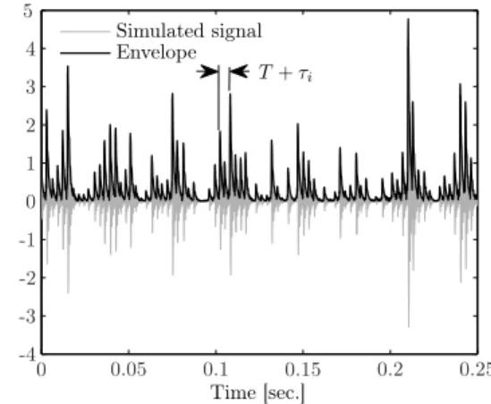
The definition of SK given by the Eq.(9) bears resemblance with the statistical definition of kurtosis. However the actual physical interpretation and its ability for detection of non-stationary transients in signals is not so obvious. One way for clarification is to observe the time–frequency characteris-tic of the simulated vibration signalx(t), defined by Eq. (5). The simulation was conducted with T = 333 Hz, s(t) =
e−100tsin(2π1500t)and SNR=1. The random time
fluctu-ationsτi and random amplitudesAi were Gaussian random processes with zero–mean withστi = 0.05T andσAi = 0.5 respectively (cf. Figure 1).
Time [sec.] Simulated signal Envelope
T+τi
0 0.05 0.1 0.15 0.2 0.25 -4
-3 -2 -1 0 1 2 3 4 5
Figure 1. Simulated signalx(t), Eq. (5)
The time–frequency characteristic of the simulated signal is shown in Figure 2. It is noticeable that the highest peaks are around 1.5 kHz, which was the chosen simulated eigenfre-quency of the impulse responses(t). The amplitudes of the spectral components around 1.5 kHz vary in time consider-ably, compared to the ones above and below this frequency band. By calculating the average over time we will obtain the standard power–spectral density (PSD).
Frequency [Hz] Time moments [sec.]
0 1000
2000 3000
4000 5000 0.1
0.2 0.3 0.4 0.5
10 20 30
Figure 2. Time–frequency characteristic of the simulated sig-nalx(t)Eq. (5)
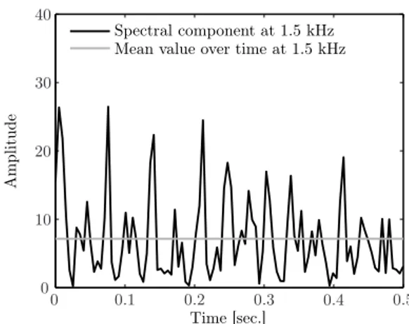
If we now consider the changes of the amplitude of particu-lar spectral components as a stochastic process, the spectral kurtosis actually searches for the frequency band where this stochastic process exhibits the highest kurtosis. For our simu-lated signal Eq. (5), the frequency band in question is around the resonance frequency of 1.5 kHz. The time change of the amplitude of that spectral component compared with its aver-age value is shown in Figure 3.
Time [sec.]
A
m
p
li
tu
d
e
Spectral component at 1.5 kHz Mean value over time at 1.5 kHz
0 0.1 0.2 0.3 0.4 0.5 0
10 20 30 40
Figure 3. Changes of amplitude of the spectral component at 1.5 kHz over time
discrepancies in amplitude of some spectral components in time will be more expressed then in the cases of stationary processes. Consequently, we can use the SK as an indicator for a frequency band where the signal’s non–stationarities are most expressed.
The estimation of the time–frequency characteristics of the simulated signal was based on the Short–time Fourier trans-form (STFT). Since the resolution in time and in frequency depends on the used window length, the search for the best frequency range is performed by examining the SK value for several window lengths (Antoni, 2007). This procedure pro-duces a diagram calledkurtogram. The kurtogram diagram for the simulated signalx(t)defined by Eq. (5) is shown in Figure 4.
Frequency [Hz]
N
u
m
b
er
o
f
fi
lt
er
s
0 1000 2000 3000 4000 0 0.2 0.4 0.6 0.8 1 1.2 1.4 0
2
4
6
8
10
12
14
Figure 4. Kurtogram of the simulated signalx(t)defined by Eq. (5)
From the kurtogram shown in Figure 4, we can see that the maximal value of SK is obtained in the frequency band with central frequencyfc = 1500Hz and bandwidthBw = 625Hz, and the maximum of SK in that frequency band is 1.4.
For a comprehensive derivation and all properties of SK one
should refer the following references (Antoni, 2006; Antoni & Randall, 2006; Sawalhi et al., 2007).
3.2 Envelope analysis
After filtering the signal in the frequency range determined by the SK method, the final step in the fault detection process is done by envelope analysis. The use of envelope analysis is justified, because the information about the fault is in the occurrence periodT of the quasi–periodic impact impulses. For the simulated signalx(t)defined by Eq. (5), the envelope is marked with black line in Figure 1.
The signal’s envelope is obtained from the Hilbert transform, i.e. by analyzing the amplitude of the analytical signalxa(t). The analytical signalxa(t) is a complex signal whose real part is the original signalx(t), and the imaginary part is the Hilbert transform of the original signalx(t)
xa(t) =x(t) +iH[x(t)], (10)
whereH[x(t)]is the Hilbert transform of the signalx(t)
H[x(t)] = 1
2π
Z +∞
−∞ x(t)
t−τdτ. (11)
Fourier transform of the analytical signalxa(t)is:
Xa(t)(f) =X(f) +jH[X(t)]
=
2X(t) forf >0, X(t) forf = 0, 0 forf <0.
(12)
This shows that the analytical signal has spectrum only in the positive frequency range. By calculating the amplitude of the analytical signal (10)
a(t) =px2(t) +H2[x(t)] (13)
we obtain the envelope of the signal.
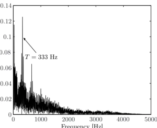
The spectrum of the envelope of the simulated signalx(t)is shown in Figure 5. From that spectrum we can easily identify the spectral component at 333 Hz, which is the period of the occurrence of the simulated impacts.
Frequency [Hz] T= 333Hz
0 1000 2000 3000 4000 5000
0 0.02 0.04 0.06 0.08 0.1 0.12 0.14
Figure 5. Envelope spectrum of the simulated signalx(t), defined by Eq. (5)
This procedure will be presented by analyzing the envelope of an amplitude modulated (AM) signalyam(t)in form:
yam(t) = [C+m(t)]cos(ωct)
=y0(t)cos(ωct), (14)
wherey0(t) = [C+m(t)]is the modulation signal, or the envelope, andωc= 2π/Tcis the carrier frequency.
The Fourier transform of the absolute value|yam(t)|can be obtained as
F{|yam(t)|}=X p
Z
Tp
yam(t)e−jωtdt
−X q
Z
T q
yam(t)e−jωtdt
=F{yam(t)}(ω)
−2X q
Z
T q
yam(t)e−jωtdt,
(15)
whereTpis one of the intervals where the signaly(t)is pos-itive, andTqis one of the intervals wherey(t)is negative. In lower frequenciesω0 < ωmax, the spectrum of the observed signal is zero, i.e. F{yo(t)}(ω) = 0,∀ω ≥ ωmax, where 0< ωmax≪ωc. Under these conditions the Eq. (15) can be rewritten as
F{|yam(t)|}(ω0) =
=−2X q
Z
T q
yam(t)e−jω0t dt
=−2X q
Z
T q
[C+m(t)]cos(ωct)e−jω0t dt.
(16)
If we now allow ωc → ∞, the intervals Tq will tend to zero, and within the observed interval the function [C + m(t)]cos(ωct)e−jω0t
may be considered as constant. The ob-served value is the value of the function in momenttq, which
is the middle of the Tq interval. Under these assumptions Eq. (16) becomes
lim
ωc→∞F{|yam(t)|}(ω0) =
=−2X q
[C+m(tn)]e−jω0tn Z
T q
cos(ωct)dt=
=−2X q
[C+m(tn)]e−jω0tn
− 2 ωc
=
= 2X
q
[C+m(tn)]e−jω0tnTc
π.
(17)
Since we have allowed ωc → ∞, consequently the period
Tc →0. In such case we can change the summation to inte-gration and the Eq. (17) becomes
lim
Tc→0F{|yam(t)|}(ω0) = 2 π
Z
[C+m(t)]e−jω0tdt. (18)
The last part of Eq. (18) is actually the Fourier transform of the signals envelope. Finally we can conclude that when
ω0≪ωcthen
F{|yam(t)|}(ω0)∝ F{C+m(t)}(ω0). (19)
4. FAULT DETECTION PROCEDURE
Traditionally, the presence of fault is determined based on a results of a spectrum comparison with previous data (fault– free data) (Sawalhi & Randall, 2008). Since such set of fault– free data was unavailable, we had to use a different approach in order to detect the faulty experimental runs. We have adopted a two step approach. Firstly we have constructed a set of experimental runs that are most likely to represent a run with faulty element. As a second step, each of these presum-ably faulty runs was analyzed using envelope spectra of the filtered signal in the frequency band that maximizes the SK value.
damage. So SK value was calculated for each measurement separately and the measurements were sorted by decreasing values of SK. Thus, the measurements at the top of the list were more likely to represent faulty runs, and those at the bot-tom of the list were considered as more likely to be fault–free runs.
In the second step, the fault isolation procedure, started by analyzing measurements from the top of the sorted list. Each signal from the list was filtered in the frequency band in which the value of SK was the highest. After that the envelope spec-trum of such filtered signal was calculated by applying the Eq. (19), although one might also opt for the calculation of the signal’s envelope based on Hilbert transform and Eq. (13). The fault detection was based on the amplitudes of spectral components at the bearing characteristic frequencies, defined by Eq. (1), obtained from the envelope spectrum. A block diagram of the described approach is shown in Figure 6.
Calculation of Envelope Spectrum Select measurements
with maximal SK Calculation of Kurtogram diagram
START
Analysis
Select measurement with next biggest value of SK
END
Selected SK larger than threshold? YES
NO
Figure 6. Block diagram of the used fault detection algorithm
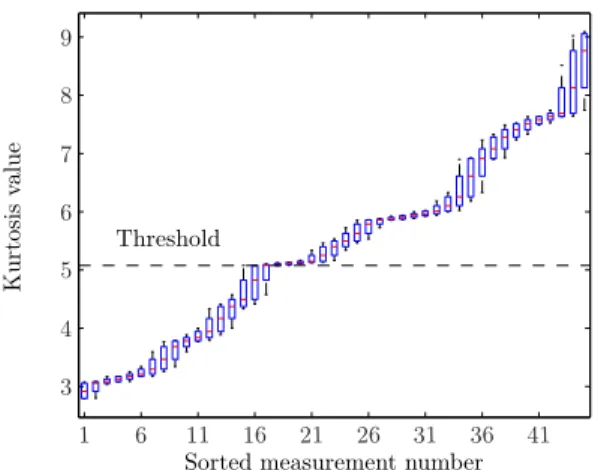
After the analysis of all experimental runs from the top of the list, the next step is to determine whether the remaining mea-surements consist of only fault–free runs. In this is the case the algorithm ends. The decision whether the remaining runs contain experiments with damaged elements is based on the value of SK. The values of SK for a group of 112 measure-ments for one particular speed is shown in Figure 7. Under assumption that the fault–free runs have the smallest value of
SK, we can determine a threshold that can serve as a boundary between faulty and fault–free runs. The procedure for selec-tion of the threshold takes into account the fact that SK val-ues for multiple measurements with same kind of fault should have similar values. Therefore, if we take a window consist-ing of several neighborconsist-ing measurements and calculate the interquartile interval on their SK values, we can use the width of the interquartile interval to determine whether the measure-ments originate from the same machine configuration or not. If they do originate from the same configuration, the width of the interquartile interval will be smaller. Otherwise it will be significantly larger. Thus, we can use the width of interquar-tile interval as an indication which neighboring measurements have been done in different machine configuration.
The first change in the machine configuration occurs when some kind of fault was introduced into a fault–free machine. In order to identify this change we analyzed the interquar-tile intervals of the measurements with lowest value of SK. The values of the interquartile intervals are shown in Figure 8 using a box plot. From the figure we can detect that the mea-surements with the smallest width of the interquartile interval are found for measurements 18,19 and 20. This leads to a con-clusion that the first change in the machine configuration oc-curred several measurements before i.e. somewhere between the 14th and the 17th measurement. In this interval the 16th measurement has the widest interquartile interval. Therefore, as a threshold we have chosen the upper interquartile value of the 16thmeasurement.
Measurment number
V
a
lu
e
o
f
S
p
ec
tr
a
l
K
u
rt
o
si
s
0 20 40 60 80 100 120 0
200 400 600 800 1000 1200
Figure 7. Values of the spectral kurtosis for 112 measure-ments
K
u
rt
o
si
s
va
lu
e
Sorted measurement number Threshold
1 6 11 16 21 26 31 36 41 3
4 5 6 7 8 9
Figure 8. Box plot for the values of SK for determining the threshold (only the lower values of SK are depicted)
the overall fault detection process.
4.1 Results
The values of SK for a batch of 112 measurements with same speed is shown in Figure 7. We can notice that some mea-surements show high values of SK compared to the rest of the batch. As already explained, the iterative procedure starts with the measurement that has the highest SK.
The kurtogram diagram for the experimental run with the highest kurtosis is shown in Figure 9. In this particular case, the frequency band with the highest SK can be ob-tained by filtering the original signal with a band–pass filter with central frequencyfc = 18.7kHz and filter bandwidth
Bw= 1.4kHz.
Frequency [kHz]
N
u
m
b
m
er
o
f
fi
lt
er
s
0 5 10 15 20 25 30
200 400 600 800 1000 0
2 4 6 8 10 12 14 16 18 20 22
Figure 9. Kurtogram for the measurement from the top of the sorted list
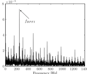
By using this filter parameters we calculated the envelope spectrum of the examined measurement, shown in Figure 10. The envelope spectrum is dominated by a single spectral com-ponent atfBP F I.
Since the spectrum is dominated by a single spectral compo-nent the fault diagnosis procedure is fairly simple. However,
Original signal
Time [sec.]
Envelope spectrum of the filtered signal
Frequency [Hz] fBP F I
0 200 400 600 800 1000 1200 1400
0 0.5 1 1.5 2
0 0.5
1×10 −7
-0.2 0 0.2
Figure 10. Envelope spectrum of the filtered vibration signal from the output shaft sensor
the final task for the data challenge was the selection which of the 6 bearings was damaged. All three shafts of the gear box rotated with different rotating speeds frot. Since all 6 bearings were of the same type, each pair of bearings on a particular shaft had its own set of bearing fault frequencies defined by Eq. (1). So, as a first step, we have located the shaft on which the faulty bearing was mounted. Afterwards, the selection which of the two possible bearings was damaged was done by observing the values of the signals acquired at both ends of the gearbox. The hypothesis is that the closer the sensor is to the fault itself the larger are the amplitudes of the corresponding bearing fault frequency. For the examined case of bearing inner race fault, the envelope spectrum of the filtered signal from the sensor mounted on the input shaft is shown in Figure 11. It is visible that the spectrum contains the spectral component atfBP F I, however the amplitude is 50 times smaller than the corresponding one from the sen-sor mounted on the output shaft, shown in Figure 10. So for this particular experimental run we can conclude that the fault was on the inner race of the bearing on the output side of the gearbox.
enve-Original signal
Time [sec.]
Envelope spectrum of the filtered signal
Frequency [Hz] fBP F I
0 200 400 600 800 1000 1200 1400
0 0.5 1 1.5 2
0 1 2 3×10⁻⁹ -0.1
0 0.1
Figure 11. Envelope spectrum of the filtered vibration signal from the input shaft sensor
lope spectrum of the filtered signal around the proposed cen-tral frequencyfcis shown in Figure 13. Similarly to the first case, the fault detection for the currently observed run is quite straightforward. The most dominant spectral component is centered atfBSF, which unambiguously points towards roller element damage.
Frequency [kHz]
N
u
m
b
er
o
f
fi
lt
er
s
0 5 10 15 20 25 30 0 1 2 3 4 0
2 4 6 8 10 12 14 16 18 20 22
Figure 12. Kurtogram for the measurement from the top of the sorted list
4.2 Procedure simplification for cases with heavy damage
Spectral kurtosis is quite efficient for cases when the tran-sient components in the measured signals have small energy compared to other vibration sources in the vicinity, like mesh-ing gears or any other environmental influence. However, for the cases where the amplitude of impulses produced by the observed fault was sufficiently high, the fault detection pro-cedure can be done by calculating the envelope spectrum of the whole unfiltered signal. Such a spectrum for the case of
fBP F I fault is shown in Figure 14. Comparing this spectrum
Original signal
Envelope spectrum of the filtered signal
frequency [Hz] fBSF
0 200 400 600 800 1000 1200 1400
0 0.5 1 1.5 2
0 1 2 3×10
−7
-0.2 0 0.2
Figure 13. Envelope spectrum of the filtered vibration signal from the input shaft sensor
with the one shown in Figure 10, we can conclude that both spectra are dominated by the same frequency component.
Frequency [Hz] fBP F I
0 200 400 600 800 1000 1200 1400
0 2 4 6 8×10
−5
Figure 14. Envelope spectrum of the unfiltered signal from the output shaft sensor
This leads to a conclusion that for cases where the severity of the fault has passed the incipient stage the use of SK, although effectual, is unnecessary. Comparably good results could be obtained by using a simple envelope analysis. Taking this finding into consideration the fault detection algorithm can be simplified, by removing the calculation of the SK for each measurement. With the removal of SK, the selection whether a particular experimental run belongs to the group of fault– free runs or not, can be done based on the amplitudes of spec-tral components of bearing principle frequencies.
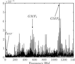
enve-lope spectrum of the unfiltered signal is shown in Figure 15. From the figure we can notice that the signal is dominated by two spectral components located at meshing gears fre-quencies, unlike the spectrum of the filtered signal shown in Figure 13 which is dominated by the spectral component at
fBSF.
Frequency [Hz] GM F1
GM F2
fBSF
0 200 400 600 800 1000 1200 1400
0 1 2 3 4 5 6×10
−5
Figure 15. Envelope spectrum of the filtered signal from the input shaft sensor
Therefore we can conclude that for experimental runs con-ducted with severely damaged bearings the calculation of SK is unnecessary. However for cases of minor damages or cases where the experimental runs were conducted under smaller loads, the calculation of SK and filtering the vibration signals prior to the analysis of the envelope spectrum is an essential step for obtaining the satisfactory results.
5. CONCLUSION
The problem of fault detection in a case when there is no ref-erence fault–free data, like in the case of the PHM Data Chal-lenge 2009, was resolved using a two step approach: combin-ing spectral kurtosis method and analysis of envelope spec-trum. In achieving our goal of bearing fault detection, the gained results of the calculation of SK were twofold. Firstly, the maximum value of SK was used as an indication whether the observed experimental run is likely to represent a run with a faulty element. Secondly, the method selects a frequency band where the impulses generated by the localized faults are most visible. This is very important step, since the amplitude of the localized bearing faults are usually significantly lower then the amplitudes of the vibrations produced by meshing gears, which effectively mask their presence. Thus a simple spectral analysis is ineffective in the process of their detec-tion. So by filtering out all other vibration influences, only spectral components originating from the localized bearing faults remain in the envelope spectrum, which additionally simplifies the fault detection procedure.
Despite all listed results, the general approach based solely on the maximal value of SK has its drawbacks. In cases of multi-ple faults, there may occur several frequency bands with sim-ilarly high values for SK. In such cases all of them should be examined and not just the one with the highest value (Combet & Gelman, 2009).
Regarding the vibration measurements obtained from PHM’09 Data Challenge, the effectiveness of SK can not be fully expressed. This is mainly due to the fact that most of the presented faults had already passed the incipient stage. As it was shown, in such cases the standard envelope analysis of the complete unfiltered signal produces satisfactory results. However, the SK pre–processing approach is effective for the cases of smaller machine loads and mild and incipient faults.
ACKNOWLEDGMENTS
The research of the first author was supported by Ad futura Programme of the Slovene Human Resources and Scholar-ship Fund. We also like to acknowledge the support of the Slovenian Research Agency through Research Programme P2-0001. The authors would like to thank Nader Sawalhi from the School of Mechanical and Manufacturing Engineer-ing, The University of New South Wales, for providing the scripts for Spectral Kurtosis.
REFERENCES
Antoni, J. (2006). The spectral kurtosis: application to the vibratory surveillance and diagnostics of rotating ma-chines.Mechanical Systems and Signal Processing,20, 308-331.
Antoni, J. (2007). Fast computation of the kurtogram for the detection of transient faults. Mechanical Systems and Signal Processing,21, 108-124.
Antoni, J., & Randall, R. (2006). The spectral kurtosis: a use-ful tool for characterising non-stationary signals. Me-chanical Systems and Signal Processing,20, 282-307. Bartelmus, W. (2001). Mathematical modelling and computer
simulations as an aid to gearbox diagnostics. Mechani-cal Systems and Signal Processing,15, 855-871. Benko, U., Petrovˇciˇc, J., Musizza, B., & Juriˇci´c, Ð. (2008).
A System for Automated Final Quality Assessment in the Manufacturing of Vacuum Cleaner Motors. In Pro-ceedings of the 17th World Congress The International Federation of Automatic Control(p. 7399-7404). Combet, F., & Gelman, L. (2009). Optimal filtering of gear
signals for early damage detection based on the spectral kurtosis. Mechanical Systems and Signal Processing, 23, 652-668.
Endo, H., Randall, R., & Gosselin, C. (2009). Differential di-agnosis of spall vs. cracks in the gear tooth fillet region: Experimental validation. Mechanical Systems and Sig-nal Processing,23, 636–651.
Ho, D., & Randall, R. B. (2000). Optimisation of bearing di-agnostic techniques using simulated and actual bearing fault signals. Mechanical Systems and Signal Process-ing,14(5), 763-788.
PHM. (2009). Prognostics and Health Man-agment Society 2009 Data Challenge. http://www.phmsociety.org/competition/09.
Randall, R. B., Antoni, J., & Chobsaard, S. (2001). The relationship between spectral correlation and envelope analysis in the diagnostics of bearing faults and other cyclostationary machine signals. Mechanical Systems and Signal Processing,15, 945 - 962.
Rubini, R., & Meneghetti, U. (2001). Application of the en-velope and wavelet transform and analyses for the di-agnosis of incipient faults in ball bearings.Mechanical Systems and Signal Processing,15(2), 287-302. Sawalhi, N., & Randall, R. (2008). Simulating gear and
bear-ing interactions in the presence of faults Part I. The combined gear bearing dynamic model and the simu-lation of localised bearing faults. Mechanical Systems and Signal Processing,22, 1924-1951.
Sawalhi, N., Randall, R., & Endo, H. (2007). The enhance-ment of fault detection and diagnosis in rolling eleenhance-ment bearings using minimum entropy deconvolution com-bined with spectral kurtosis. Mechanical Systems and Signal Processing,21, 2616-2633.
Staszewski, W. J. (1998). Wavelet based compression and feature selection for vibration analysis. Journal of Sound and Vibration,211, 735 - 760.
Tandon, N., & Choudhury, A. (1999). A review of vibration and acoustic measurement methods for the detection of defects in rolling element bearings. Tribology Interna-tional,32, 469-480.