herwig immervoll§ horácio levy¤ José ricardo nogueira† cathal o’donoghue ‡ rozane Bezerra de Siqueira
reSumo
Apesar de arrecadar um montante de tributos equivalente a cerca de 37% do PIB e gastar mais da metade desta receita em programas sociais, o governo brasileiro não tem sido capaz de aliviar significativamente o problema da desigualdade e da pobreza. Alguns estudos têm mostrado evidência de que esta situação é, em grande parte, devida à inadequada focalização dos gastos públicos. Entretanto, o impacto distributivo do financiamento desses gastos tem recebido menos atenção. O presente trabalho investiga o impacto conjunto dos tributos e transferências monetárias governamentais sobre a distribuição de renda entre os domicílios brasileiros e compara o Brasil com alguns outros países com carga tributária semelhante.
Palavras-chave: tributos, benefícios sociais, microssimulação, redistribuição, desigualdade, pobreza.
aBStract
Despite raising an amount of taxes that represents nearly 37% of the country’s GDP and spending over half of this revenue on social programmes, the Brazilian government has not been able to significantly allevi-ate inequality and poverty. A number of studies have shown evidence that, to a great extent, this situation is due to the inadequate targeting of public expenditures. The distributive impact of the financing of these expenditures, however, has received less attention. This paper investigates the combined impact of taxes and government cash transfers on the distribution of income among Brazilian households and compares Brazil’s redistributive performance with that of some countries with a similar tax burden.
Key words: taxes, socials benefits, microsimulation, redistribution, inequality, poverty.
Jel classification: H22, H23, C81.
* An earlier version of this paper was presented at the WIDER International Conference on Inequality, Poverty and Human Well Being, May 2003, Helsinki, and at the Encontro Nacional de Economia – ANPEC, December 2003, Porto Seguro. We wish also to thank an anonymous referee for useful comments. Remaining errors are ours alone.
§ ISER, University of Essex, and IZA, Bonn. E-mail: [email protected]. ¤ ISER, University of Essex. E-mail: [email protected].
† Department of Economics, Universidade Federal de Pernambuco. E-mail: [email protected]. ‡ National University of Ireland, Galway and IZA, Bonn. E-mail: [email protected].
Department of Economics, Universidade Federal de Pernambuco. E-mail: [email protected].
To contact the authors: Departamento de Economia, Universidade Federal de Pernambuco, Cidade Universitária, Recife - PE – CEP: 50.670-901.
1 i
ntroductionDespite raising an amount of taxes that represents nearly 37% of the country’s GDP and spending over half of this revenue on social programmes, the Brazilian government has not been able to significantly alleviate inequality and poverty. In fact, Brazil is among the 10 most unequal countries in the world and a large share of its population still lives in poverty. Brazil is an exception to the observed international pattern, where high income inequality is generally associated with low levels of tax revenue as a proportion of GDP. In Figure 1, we notice that the United Kingdom and Spain, for example, with a similar tax burden to that of Brazil, have a much lower income inequality as indicated by the Gini coefficient. On the other hand, Mexico and Chile, with Gini coefficients close to that for Brazil, have a much lower tax burden.1
figure 1 – tax Burden and gini coefficient
Source: Siqueira, Nogueira e Levy (2003).
To an extent, the relatively low Gini coefficients of developed countries reflect the impact of their tax-benefit systems. Evidence for this has been provided, for instance by studies that use mi-crosimulation techniques to simulate the redistributive effect of the tax and benefit systems of those countries.2 The purpose of this paper is to describe these techniques and apply them to examine the effect of the Brazilian tax-benefit system on household income and the effectiveness of govern-ment transfers in reducing poverty.
The paper is structured in five sections. After this introduction, section 2 discusses the me-thod used in this paper, microsimulation modelling. Section 3 briefly describes the taxes and cash transfers considered in this study and the main procedures and data used in our calculations. Sec-tion 4 presents and discusses the results. SecSec-tion 5 concludes.
1 The Gini index for Brazil was calculated using per capita household income; for the other countries, the indicators were ob-tained from the OECD and IMF statistical databases.
2 See, for example, EUROMOD (2004).
Netherlands Germany Canada
Australia Spain
Norway Belgium Sweden Denmark Brazil Mexico Chile Peru
Ecuador India USA UK -5 10 15 20 25 30 35 40 45 50 55 60 0,20 0,25 0,30 0,35 0,40 0,45 0,50 0,55 0,60 Gini Coefficient T o ta l T a x R e v e n u e /G D P (% ) Netherlands Germany Canada Australia Spain
Norway Belgium Sweden Denmark Brazil Mexico Chile Peru
2 S
tePStocreateataxBenefitmicroSimulationmodelIn order to evaluate the redistributional impact of the Brazilian tax-benefit system, one needs information about how taxes and benefits operate at the individual level. Because the necessary information is often not available in survey data, it is necessary to simulate these variables. For this we use a tax-benefit microsimulation model. In this section we consider the steps necessary to create a tax-benefit model.3
2.1 microsimulation modelling
Due to the great diversity observed among the population and the complexity of the Brazilian tax-benefit system, the redistributive analysis of the impact of social and fiscal policies requires that a high level of disaggregation be used in order to capture in fine detail their effects on the various types of individuals, families and households. Ultimately, it is the social and economic diversity ty-pically found in the national populations that determines how economic agents will be affected by the tax and benefit rules. On the other hand, as different social programs interact with each other and with the tax system, it is crucial to take explicitly into account the interdependencies within the whole tax-benefit system. The lack of analytical tools that properly focus on the poor and the neglect of the issue of how the programs are to be financed are major reasons why social and eco-nomic policies fail to significantly reduce poverty.
Typically hypothetical families have been used to examine the operation of taxes and benefits and impact of reforms. For example the OECD uses this method to calculate the Tax position of average Workers. Although a useful method for illustration purposes and for comparison across countries, the approach is not very satisfactory for looking at tax-benefit policy in a country as usually families which are considered “typical” form in fact only a very small proportion of the population. It is desirable therefore to look at the population as a whole using representative micro-datasets.
An approach that follows this method is microsimulation modelling. Recent advances in in-formation technology and the availability of large-scale datasets have allowed and stimulated the development of these models. Microsimulation models are computer programs that calculate tax liabilities and benefit entitlements for individuals, families or households in a nationally represen-tative micro-data sample of the population. The model calculates each element of the tax-benefit system in the legal order so that interactions between different elements of the system are fully taken into account. Calculations for each individual, family or household are weighted to provide results at the population level.
By incorporating the interactions of different elements of the tax-benefit system and by taking full account of the diversity of characteristics in the population, this approach allows a very detailed analysis of the revenue, distributional and incentive effects of the individual policy instruments and the system as a whole. In particular, they give a great deal of flexibility to analysts. For example:
They simulate policy instruments that may not already exist in the micro-datasets on which they are based. As micro-data is not necessarily collected every year and may take time for the data to be available to researchers, microsimulation models can be used to simulate more up to date policy rules.
3 In this paper we draw upon model development lessons learned by a number of the authors as part of the EUROMOD project and described in Immervoll and O’Donoghue (2001).
Therefore they have the capability of looking at the incidence of existing policy on an existing population and can examine the efficiency of anti-poverty measures in actually reducing po-verty.
As a simulation mechanism, they are also well placed to look at the incentive impact of existing policy. Although the model framework described here is a static framework, it is possible to measure the pressures on behaviour such as marginal tax rates and replacement rates.4
The primary advantage of microsimulation models however is that they can simulate policy reform. They can thus be used to compute the first round revenue effects of reforms. Also, con-taining both social protection programs and taxation instruments, models of this kind can look not only at changes to social policy programs but also examine different methods of financing. The first round distribution of resulting winners and losers, particularly with reference to par-ticular target populations, can also be found.
Capturing the heterogeneity of government law, they can examine the interaction of different policy instruments.
Incorporating micro-data, they can also be used to look at the distributional impact of policy reform. Thus it is possible to see how reforms are incident on households of different incomes, examine horizontal redistribution by focusing, for example, on families with children, the el-derly or the sick. Exploiting the hierarchical nature of households, they can also focus in gender dimensions by looking at within household sharing and the impact of government policy. The user-friendly nature of such models makes them suitable for a variety of uses and users, both governmental and non-governmental, informing the debate of social and economic policy, and making policy decisions more transparent in terms of their impacts on the population. The use of microsimulation models therefore, can greatly contribute to improved design and efficacy of policies (as argued, for instances, in Atkinson et al., 2002). The models provide a powerful aid to policy design and assessment, allowing users to consider how expenditure aimed at certain targeted groups is to be financed, how social spending is distributed among the population, and how fiscal and social policies impact on the different groups of the popula-tion. Thus, working with a microsimulation model, policy designers and analysts can simulate changes in the existing tax-benefit system, performing “what if ” experiments and examining their distributional and revenue implications. (Redmond, Sutherland and Wilson, 1998). For example, Piachaud and Sutherland (2000) recently used a microsimulation model to examine the policies necessary for the UK government to meet its poverty reduction targets.
However the development of microsimulation models is quite a difficult and expensive pro-cess. It involves the construction of a software environment to handle the data, policy simulation and output routines. The transformation and matching of existing micro-datasets into definitions and structures required to simulate tax-benefit laws and the translation of the law itself into a computational framework are quite time consuming. The latter is a very large task as instruments are often very complicated, with particular exemptions for different classes of individual or income source. Also the diverse policy instruments, having often been developed by different governmental organisations within government, may follow different logic and interact in peculiar ways.5 Ano-ther important expense is the actual updating of the model. Government policy tends to change year on year and population structures can change too due to the number of unemployed in
reces-4 See, for example, O’Donoghue and Utili (2000), who study both the distributional and incentive effects of the impact of reforms targeting low wage workers in Europe.
5 Ironically one side-effect of using tax-benefit models in a country is to help to streamline the actual tax-benefit code itself as government analysts prefer instruments which they can program more easily.
•
•
•
•
•
•
•
sions or through demographic changes. Hence in order for the model not to become out of date, efforts need to be made to update the model, both the data and the rules, in regular intervals. As a result of the expense, although a number of Western countries and institutions have utilised this technique, there is still not widespread use in emerging economies. Yet it could be argued that the benefits of these techniques could be relatively more important in emerging countries because of the greater proportions in poverty and because of their poorer public finance positions, with greater need being required in the design of effective government policy.
2.2 microsimulation modelling in developing countries
One of the issues this paper must consider are the fact that circumstances, systems and data may not necessarily be the same in developed economies, where the technique has been utilised, and in emerging economies. Atkinson and Bourguignon (1990) carried out a study of the lessons of Tax-Benefit modelling in OECD countries for emerging economies. They found that although of-ten more difficult to implement, simulating tax-benefit systems for these countries should “lead to a comprehensive, powerful and yet simple instrument for the design of an efficient redistribution system adapted to the specificity of developing countries.” Focusing on Brazil as a case study, they found that much of the redistribution in the existing Brazilian system in the 1980’s relied on instruments that were less important in OECD countries. For example, indirect taxes, subsidies and the provision of targeted non-cash benefits such as public education and subsidised school meals were found to be more important. Instruments more important in OECD systems and often the main instru-ments in tax-benefit models (personal income taxes, social insurance contributions and pensions), were largely confined to the modern sector in Brazil and thus of less importance to policy makers. Nevertheless they argued that sufficient data existed at the time to simulate many of the Brazilian specific instruments in addition to the “classic” ones. They stressed however that merging of data from different datasets may be necessary for this purpose. As a consequence of recent advances in the analysis of related data-sets (see Deaton, 1998) as well as improvements in the availability of data for less developed countries, the use of tax-benefit modelling techniques needs no longer be limited to countries where such models have been in use for some time.
Atkinson and Bourguignon’s paper set the scene for the construction of tax-benefit models for less developed countries. The objective of our study is to go beyond this and actually focus more on the practical issues of constructing a benefit model by reference to the precise rules of the tax-benefit systems and the detail of the available micro-data.
2.3 the design of a microsimulation model
A microsimulation framework adopts a hierarchical view of a country’s tax-benefit system. In modelling a country’s system, it is desirable to match the “real” system’s hierarchy as closely as possible so that the logical representation provides a good intuitive equivalent of the original.
income, then the entry Social Assistance Benefits would have to appear after Income Tax since income tax is a necessary input for calculating social assistance benefits.6 At the lowest level is the tax-benefit module, which performs the calculation of a certain part of the tax or benefit (e.g., a deduction, or applying a rate schedule to a tax base) on each fiscal unit. Only the modules contain actual tax-benefit rules. The other levels of the model are necessary to structure these rules and apply them in the correct sequence.
A modular structure allows one, as the model develops, to create a library of modules.7 These can be used as “building-blocks” so that when it is necessary to incorporate a new tax or benefit instrument, it will often not be necessary to program any new tax-benefit rules. Instead, it may be possible for existing modules to be used. They can be re-arranged in any order necessary. A high level of parameterisation ensures that the same modules can be used for a multitude of different purposes.
Concepts that a user may want to change in the model and thus should be parameterised for ease of use include:
Updating of dataset to year of simulation as the year of the dataset may not necessarily be the same as the year of simulation (the year policy rules are taken from), it will be necessary to update the dataset to account for differences in the intervening period. For this purpose ex-ternal information will be needed. Updating which may be required include, allowance for inflation/income growth by variable or allowance for changing population structure by altering the weights.
The definition of the fiscal unit (e.g., individual, household, married couple, families with chil-dren – including the definition of a “child”) which is relevant for the module,
Income concepts (e.g., the definition of taxable income, “means” for a means-tested benefit, etc.). In order to simulate the effect of widening the tax base or of incorporating new policies in a particular income concept such as disposable income, users may want to alter with ease the definition of these concepts.
All relevant amounts (such as thresholds, limits, allowances, rates, number of tax bands, etc.) necessary for applying the relevant tax or benefit rules should be parameterised to enable non-structural policy reforms to be simulated with ease.
Behavioural response
Behavioural Response and Sensitivity Analysis. As a static modelling framework, the model only measures the day after effect. However it is clear that reforms may have a behavioural res-ponse. For example the introduction of the Bolsa Escola program in a number of Brazilian cities which gives cash benefits to poor families whose children continue on in school until 14, saw school dropout rates decrease and school attendance increase. (Schiefelbein, 1997). Thus the cost of the program would have been higher than a static analysis would have indicated. Incorpora-ting dynamic processes like this would be beyond the scope of an initial stage of construction of a microsimulation model. It would require extra algorithms to be coded in the framework and in addition, a priori, the micro-behavioural information required would not have been available for a reform of this kind. However, as an alternative, sensitivity analyses could be carried out. It would be possible for analysts to vary the proportion of those eligible for the new instrument. Routines of
6 In a few cases, it might be desirable to deviate from a purely linear sequence of policies. If there are optional policies, which the tax payer/benefit recipient can choose from, it would be necessary to simulate all the individual options (e.g., individual or joint taxation) and then apply some rule for choosing between them (e.g., by assuming a decision which would maximise disposable income).
7 In a national model one builds up a library of historic instruments and reforms that were experimented with. •
•
•
this kind are analogous to the implementation of marginal tax-rate calculators. On this point some effort may also be necessary to specify appropriate definitions of marginal tax calculations in the framework for a Brazilian perspective.
validation
Once the tax-benefit system has been coded the data are passed through the model. At this stage, one discovers whether all the variables required by the model algorithms have in fact been included in the dataset and whether they are in the correct format. Once this works, one must de-termine whether all the interactions between the simulated components operate correctly. The va-lidation process is therefore one of the largest components in building a microsimulation model.
Typically the first stage in this process is to compare the output of the model for sets of hypo-thetical households against manually calculated taxes and benefits. Although the rules may in fact be correctly coded, simulated aggregates may not necessarily match official aggregates. The next stage of the validation process is therefore to compare the aggregate outputs against those in official statistics. Useful external sources of data for validation include official figures, other studies, other survey data, existing models, etc.
3 B
uildingthePrototyPeIn this study we implement a prototype tax-benefit microsimulation model for Brazil, the Brazilian Household Microsimulation System (BRAHMS). The model simulates household sector taxes and cash transfers based on the 1999 household survey pesquisa nacional por amostra de
Do-micílios – PNAD.8 The PNAD is the main microdata source of demographic and socio-economic
household characteristics in Brazil. It is a nationally representative rural-and-urban survey covering all Brazilian regions with the exception of the North region’s rural area. PNAD’s sample size is quite large, including more than 100,000 households and more than 300,000 individuals. However, PNAD does not contain expenditure data. Information for household expenditure comes from the pesquisa de orçamentos Familiares (POF) 1995/96, Brazil’s main expenditure survey.
The major direct and indirect taxes are simulated in the model.9 The taxes that are simulated by the model include the following income based revenue raising instruments:
Personal income tax,
Employee and the employer social security contributions.
In the case of the personal income tax and the social insurance contributions, for which there is no direct information in the PNAD, the values are simulated applying the legislation of the tax system to each individual or family in the PNAD microdata set. The estimates are then compared to available administrative data and adjusted to better reflect the effective incidence on taxes and benefits. The simulated amounts, validated against administrative data were found, on average, to be about 90% of the administrative data.
In addition the following indirect taxes are also simulated: Taxes on the circulation of goods and services (ICMS), Taxes on industrialised products (IPI),
8 Currently, the model is being prepared to incorporate the PNAD 2004 as the main dataset. 9 See Table A.2 in the Appendix for a description of these taxes.
• •
Contribution to the financing of the social security (COFINS).
Because there are no expenditure data in the PNAD and because of the time limitations in the present study preventing us from doing a statistical match between the datasets, an imputation mechanism has been used to simulate indirect taxes.
The amount of indirect taxes paid by households was calculated as follows:
The effective tax rates on final goods and services were estimated using input-output techni-ques;10
The estimated tax rates were applied to the 1995/96 household expenditure survey pesquisa de orçamentos Familiares – POF to calculate the amount of indirect taxes paid by POF households as a proportion of their incomes;
These proportions were then used to estimate the payment of indirect taxes by the PNAD hou-seholds groups defined in this paper.
It should be noted that, since POF covers only metropolitan areas, the procedure described above to impute indirect taxes assumes that the tax burden on a household elsewhere in the country is the same as that on a metropolitan household with the same income. In addition, it is assumed that the definitions of income in POF and PNAD are compatible.
BRAHMS simulates the following cash transfer programs:11 The old age assistance benefit, the unemployment benefit, the wage bonus, the family benefit (salário-família) and the
Bolsa-Es-cola programs.12 For the Bolsa-Escola programs, we have opted in the present paper to simulate the
coverage defined in the 2002 Federal Government budget rather than the 1999 situation. This is because expenditure on these programs has increased drastically since 1999 (yet it still represents only about 2% of the total benefits allocated in this paper). Thus, the benefits of these programs were imputed in our data on the basis of their 2002 coverage, with values deflated to 1999.13
On the other hand, pensions (regarding both the civil servant and private employee regimes) are taken directly from the PNAD. While for the incidence analysis conducted in this study it is not necessary to simulate these transfer instruments, future analysis of potential reforms will require this. However as is common in static microsimulation models, the simulation of contribution-based old age pensions is often difficult due to a lack of data on past income and years of contribution.
4 r
eSultSIn this section we use the BRAHMS model to describe the incidence of different types of government transfers and taxes on households. To do this, we use a set of income concepts. The starting point is initial income, which is the total annual income of all members of the household before the deduction of taxes or the addition of any social benefits. Cash benefits are added to initial income to obtain gross income. Personal income tax and employers and employees
contribu-10 Details on the methodology are presented in Siqueira, Nogueira and Souza (2001), where it is assumed that indirect taxes are fully shifted to the final consumer.
11 See Table A.1 in the Appendix for a description of these benefits.
12 The Bolsa Escola programs are cash transfer schemes targeted at families with children, conditioned to school attendance for school-aged children. Here the term actually refers to three different programs, the Bolsa Escola, the Bolsa alimentação, and the
Bolsa criança cidadã, which were grouped together for purpose of presentation in this paper.
13 A set of social expenditure items that so far have not been included but which are often relatively more important in developing coun-tries is non-cash social spending, such as health and education benefits. This is especially important for households outside the modern sector as they are often excluded from coverage of social security benefits. This is another future development of this model. •
1.
2.
tions to social security are deducted from gross income to give disposable income. Indirect taxes are then deducted to compute final income.
4.1 total redistribution
As said in section 1, the relatively low levels of income inequality of developed countries found in Figure 1, to an extent, reflect the impact of their tax and benefit systems.14 By contrast, Brazil has not been able to use tax and transfers policies effectively to reduce income inequality. This is illustrated in Table 1, which summarises the estimated impacts of cash transfers and direct taxes on the distribution of income in Brazil.15 It shows that the richest 10% of households (according to equivalent gross income) receive 45.9% of all initial income. This compares with only 0.7% for households in the bottom tenth.
table 1 – Percentage shares of household income, ratios of share of the top 20% to share of bottom 40% and gini coefficients
Household Groups (Ranked by Gross Income)
Percentage share of income
Initial Income
Gross Income
Disposable Income
Final Income
Bottom 0.7 0.8 1.0 0.9
2nd 1.5 1.7 1.9 1.8
3rd 2.3 2.5 2.7 2.5
4th 3.2 3.4 3.6 3.4
5th 4.2 4.5 4.6 4.4
6th 6.0 5.9 6.0 5.6
7th 8.2 8.1 8.1 7.7
8th 11.3 10.9 10.9 10.5
9th 16.7 16.5 16.5 16.5
Top 45.9 45.7 44.8 46.6
All households 100 100 100 100.0
Ratio of share of top 20%
to bottom 40% 8.1 7.4 6.7 7.3
Gini coeficient 0.642 0.581 0.564 0.579
Notes: 1. Households are ranked by income per adult equivalent, where the equivalence scale used is 1 for the principal adult, 0.7 for other adults, and 0.5 for children aged under 18.
2. Initial income: total annual income of all members of the household before the deduction of taxes or the addition of any state benefits.
3. Gross income: initial income plus state benefits.
4. Disposable income: gross income minus direct taxes and contributions. 5. Final income: disposable income minus indirect taxes.
The distribution of gross income, which includes government cash transfers, shows a very similar pattern as the distribution of initial income. In particular, the top tenth’s share remains virtually the same (45.7%), while the share appropriated by the first tenth remains below 1.0%. Thus, there is only a small reduction in ratio of the income share of the top 20% to the share of the
14 See, for instance, Beer et al. (2001).
bottom 40%, from 8.1 to 7.4. It should be stressed, however, that the distribution of initial income shown in Table 1 is among households ranked by gross income, which gives a less regressive picture than if households were ranked by initial income, for, as we shall see below, pension benefits pro-duce a significant reranking of households. In this case, the concentration of initial income is better captured by the Gini index, which is substantially lower than that of gross income.
The third column of Table 1 shows that the personal income tax and the employer and em-ployee social security contributions, altogether, reduce the share of the richest 10% to 44.8% and increase the share of the poorest 10% to 1.0%. This effect reflects the fact that almost all personal income taxed (97%) and about 38% of social security contributions are collected from the top tenth, while the average burden of direct taxes on the first tenth is insignificant.
The final column of Table 1 incorporates the impact of indirect taxes. As we shall see below indirect taxes are regressive and so the gap between rich and poor widens as the richest tenth now receives 46.6% of all final income and the richest fifth receives 7.3 times the final income of the poorest fifth compared with 6.7 times for disposable income. Thus indirect taxes essentially cancel out the progressive effect of direct taxes, as also indicated by the change in the Gini index.
4.2 Progressivity of individual instruments
In this section, we consider the redistributive effect and the progressivity of the individual instruments of the tax-benefit system. We use measures based on the Lorenz Curve to examine the degree of redistribution and progressivity.16 The Lorenz Curve for pre-tax market income (lM) is simply a graph of the cumulative population share versus the cumulative income for the population ranked by order of their income. The Gini coefficient is a standard index of inequality, defined in equation (1):
1
0
1 2 ( )
M M
G = −
∫
L p dp (1)where p is the cumulative population share and LM(p), the Lorenz Curve at point p.
A population with no income inequality would have a Lorenz Curve of 45° and therefore a Gini of 0. If Lorenz Curve 1 lies completely outside curve 2, then it is possible to say that popula-tion 1 has greater inequality than populapopula-tion 2, with G1 > G2. However if the Lorenz Curves cross, it is not possible to make inequality comparisons without using further value judgments.
The index used here to measure redistribution is the Reynolds-Smolensky index, which is defined as the difference between the Gini coefficients for “base” income (defined here as initial income M) and post-instrument income (M’):
L = GM – GM’ (2)
Progressivity is a measure of the difference between the level of redistribution of an instru-ment relative to an instruinstru-ment with the same revenue effect but where the effect is proportional to income. It is therefore a measure of the incidence of an instrument. If an instrument is dispropor-tionally focused on the lower (upper) half of the distribution, then it is regressive (progressive). If an instrument is regressive (progressive), the concentration curve for the instrument will fall inside
(outside) the Lorenz curve of market income. If the instrument is proportional to income, the con-centration curve will be exactly the same as the Lorenz curve for market income.
In terms of income taxes, progressivity relates to the ability-to-pay principle, whereby those with higher incomes are more able to pay higher taxes. A progressive income tax is therefore re-distributive and thus inequality reducing. On the other-hand, benefits are rere-distributive if they are regressive, so that those with lower incomes receive higher benefits.
In this paper we use the Kakwani index of progressivity, defined as:
K = CT –GM (3)
where cTis an index similar to the Gini measure, being derived from a curve, called concentration curve of the instrument T, in which the individuals are ordered according to their initial incomes, and the proportion of the population is related to the corresponding proportion of the instrument (tax paid or transfer received) incident on those individuals.
If policy instruments are based on characteristics other than income, then income units may have a different order of incomes before and after the operation of the instrument. For example pensions are targeted at households with elderly people and so households with elderly people will receive subsidies while other households will not. This type of redistribution is known as horizon-tal redistribution. Changes in the order of income units in a distribution will result in the Lorenz curve of post-instrument income being different from its concentration curve. The Atkinson-Plot-nick reranking index is the measure of horizontal equity we use, defined as:
P = (GM’ – CM’)/2GM’ (4)
The concentration index, cM’, involves ranking by M and the Gini inequality index, GM’, invol-ves ranking by M’, so that an absence of re-ranking implies that p = 0. (Creedy, 1997).
The redistributive effect of a policy instrument depends upon the size of the instrument and the progressivity or degree of targeting. For example, a well-targeted low value instrument may have a lower degree of redistribution than a poorly-targeted high value instrument.
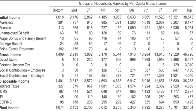
The average amounts of taxes paid by each household group are shown in Table 2. Although the income tax is usually at the centre of the tax policy debate in Brazil, one can observe that it is indirect taxes and payroll taxes that account for most of the tax burden borne by households; per-sonal income taxes only account for 3.7% of initial income compared with total taxation of 31.1%. Personal income tax is important only to the households in the top tenth, representing, in average, 6% of their gross income.
table 2 – average incomes, taxes and transfers by household group, Brazil – 1999 (r$ per year)
Groups of Households Ranked by Per Capita Gross Income
Bottom 2nd 3rd 4th 5th 6th 7th 8th 9th Top
Initial Income 1,018 2,176 2,862 4,185 3,953 6,633 8,665 11,523 16,321 38,543
Transfers 391 737 940 985 1,391 1,280 1,619 2,087 3,207 8,177
Pension 113 365 618 727 1,152 1,090 1,421 1,923 3,035 8,054
Unemployed Beneit 63 75 80 120 69 76 111 89 116 57 Wage Bonus and Family Beneit 10 65 93 116 74 106 87 76 57 66
Old Age Beneit 24 53 80 17 96 7 0 0 0 0
Bolsa-Escola Programs 182 179 70 4 0 0 0 0 0 0
Gross Income 1,409 2,913 3,802 5,170 5,344 7,913 10,284 13,610 19,528 46,720
Direct Taxes 8 101 230 477 506 996 1,368 1,953 2,898 8,457
Personal Income Tax 0 0 0 0 0 1 4 8 129 3,010
Social Contribution – Employee 3 30 61 126 133 274 387 588 847 1,406
Social Contribution – Employer 5 71 168 351 373 721 977 1,357 1,921 4,040
Disposable Income 1,401 2,812 3,572 4,693 4,838 6,917 8,916 11,657 16,630 38,263
Indirect Taxes 327 679 867 1,081 1,085 1,574 1,924 2,382 2,929 4,859
ICMS 197 411 521 646 647 965 1,183 1,429 1,777 2,897
IPI 45 90 110 140 139 182 206 259 293 467
COFINS 85 178 236 295 299 427 535 694 859 1,495
Final Income 1,074 2,133 2,705 3,612 3,753 5,343 6,992 9,275 13,701 33,404
Reflecting progressivity patterns found throughout the world, personal income taxes are the most progressive of the taxes, with a Kakwani index of 0.251. The social security contributions sho-wn in Table 2 include those paid by employees and employers, assuming that the latter shift the tax on to the former through lower wages. Overall, the burden of social security contribution borne by households is higher than the income tax burden, even for the richest tenth. Social insurance con-tributions are progressive but less so (0.023 for employee and 0.044 for employer concon-tributions) than the personal income tax system. From Table 2 we can infer that social contributions as a percentage of initial income increases up to the seventh household group, falling in the top tenth. This reflects the existence of a ceiling in the contribution of private employees. One should also note that the low level of social security contribution in the lowest income groups reflect the fact that there is a sizeable proportion of informal workers in these groups.
Indirect taxes are levied on consumption and because poorer households tend to have lower savings rates than richer households, they consume a higher proportion of their income and so pay proportionally more indirect taxes. As a result indirect taxes have a regressive effect. However, the income saved today by the rich will be spent in a future date, when it will then be taxed. Thus, to measure the incidence of indirect taxes in terms of current income tend to overestimate the regres-sivity of these taxes.17 However, independently of how the indirect tax burden varies among the income groups, it is important to stress that the burden borne by the low-income groups in Brazil is quite high, representing about one quarter of the consumption spending of the poorest 10% hou-seholds (Table 2).
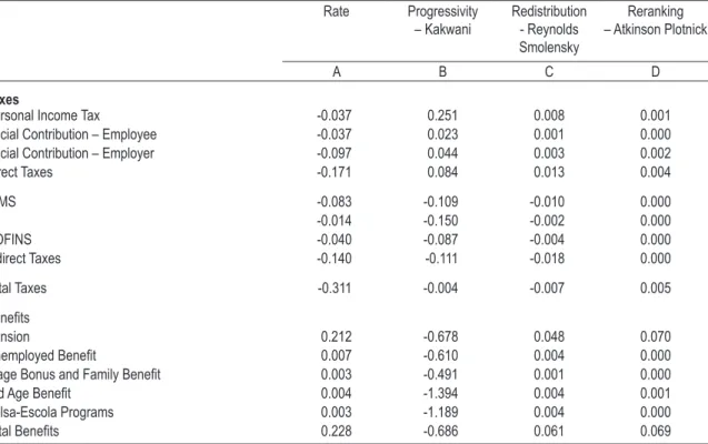
table 3 – Progressivity and redistributive effect of the Brazilian tax-benefit instruments
Rate Progressivity
– Kakwani
Redistribution - Reynolds Smolensky
Reranking – Atkinson Plotnick
A B C D
Taxes
Personal Income Tax -0.037 0.251 0.008 0.001
Social Contribution – Employee -0.037 0.023 0.001 0.000
Social Contribution – Employer -0.097 0.044 0.003 0.002
Direct Taxes -0.171 0.084 0.013 0.004
ICMS -0.083 -0.109 -0.010 0.000
IPI -0.014 -0.150 -0.002 0.000
COFINS -0.040 -0.087 -0.004 0.000
Indirect Taxes -0.140 -0.111 -0.018 0.000
Total Taxes -0.311 -0.004 -0.007 0.005
Beneits
Pension 0.212 -0.678 0.048 0.070
Unemployed Beneit 0.007 -0.610 0.004 0.000
Wage Bonus and Family Beneit 0.003 -0.491 0.001 0.000
Old Age Beneit 0.004 -1.394 0.004 0.001
Bolsa-Escola Programs 0.003 -1.189 0.004 0.000
Total Beneits 0.228 -0.686 0.061 0.069
Note: 1. All incomes have been equivalised using the scale described in Table 1.
2. The base income used is initial income. In other words, the progressivity of an income is expressed relative to the progressivity of initial income. The rate refers to the instrument as a proportion of initial income and redistribution measures the change in the distribution of income through the inclusion of the instrument in question.
Combining the size of the instruments (column A) with the knowledge we have about their progressivity (column B), we can determine how redistributive each instrument is. Personal in-come taxation although of relatively low importance, has the highest redistributive effect, driven primarily by the strength of the progressivity effect. However, because indirect taxes are regressive and because they are of greater importance than direct taxes, the total redistributive effect of taxes is marginally negative. In Table 1 where we report the Gini for gross and final incomes, we see that the net impact of taxation is marginally positive in reducing inequality. The difference results from a different base for comparison (initial income versus gross income). However, the direction of redistribution in either case is very small and so we can therefore conclude that taxation is ap-proximately neutral.
eliminated by this reranking, with pensions, as a proportion of income, distributed fairly evenly across household groups with a peak in the centre of the distribution.
Unemployment benefits are the next biggest transfer group, with progressivity similar to that of pensions. Reranking is hardly present. Wage bonus and family benefits are the least targeted transfers. On the other hand, old age and Bolsa Escola instruments, because they are not restricted to households in the formal sectors, are potentially very targeted, with Kakwani indices of respec-tively –1.394 and –1.189. It should be stressed that our simulations of Bolsa Escola programmes do not take into account target imperfections due to administrative and take-up problems, meaning that they are run under the assumption that all the recipients of the benefit satisfy the eligibility criteria.
Turning to the redistributive impact of the instruments, we see that on the whole redistribu-tion is quite small, reducing inequality by about 6% points. Most of this is driven by the pension system. However as per the discussion above, we note the degree of reranking due to the system.
4.3 comparison with other countries
How does the redistribution observed in Brazil compare with redistribution in other coun-tries? In this section we contrast redistribution in Brazil with that observed in a number of Indus-trialised countries.18
Figure 2 describes the Gini coefficient for different income concepts for the sixteen countries considered. The size of the levelling of income distribution through the benefit and tax system can be measured by means of the Gini coefficient. The difference between the Gini coefficients of the different income concepts is indicative of the degree of redistribution inherent in the difference between incomes. We notice that the reduction in the Gini coefficient due to benefits (moving from initial to gross income) and due to direct taxes/contributions (moving from gross to disposable income) is much smaller in Brazil than in the other countries. While direct taxes have a relatively small redistributive effect on the Industrialised countries, reducing the Gini coefficient by 5-6 percentage points, in Brazil the effect is even smaller, at less than 2 percentage points. The biggest difference however is in the lack of redistributive power in the benefit system. While it is the most important set of redistributive instruments in Brazil, reducing the Gini coefficient by 6 percentage points, it has a much smaller effect than instruments in the Industrialised countries, where with the exception of the USA and Australia, there are reductions of 14-20 percentage points. Even the industrialised countries with lowest redistribution, Australia and the United States, have double the reduction of Brazil. Therefore it is the lack of redistributive power in the transfer system that primarily drives the lower redistribution in Brazil compared with other countries.19
18 See Baldini, O’Donoghue and Mantovani (2004).
figure 2 – the reduction in the gini coefficient due to direct taxes and benefits
0,000 0,050 0,100 0,150 0,200 0,250 0,300
Br Fr Gr It Pt S p S w Dk No Nl Ge Be Ca UK Au US A
G
in
i R
ed
u
cti
on
Taxation
Benefits
Source: Baldini, O’Donoghue and Mantovani (2004) and Beer et al. (2001).
4.4. Poverty efficiency of Benefits
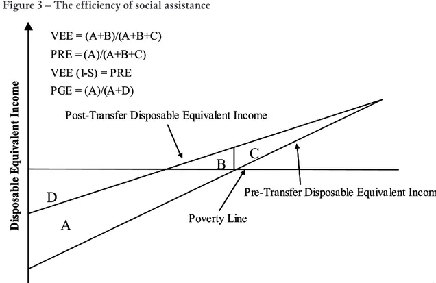
Although the reduction of income inequality is one of the objectives of taxation and transfer systems, a more focused objective is the reduction of poverty. Here we consider how effective Bra-zilian transfer instruments are at reducing poverty. In Table 4 we describe a number of measures (see Weisbrod, 1970; Beckerman, 1979) of the poverty efficiency of transfers in Brazil compared with means-tested instruments in Southern European countries, as reported in O’Donoghue et al. (2003), for each of the schemes mentioned before. Figure 3, due to Beckerman (1979), describes the impact of transfers on disposable income. The measures we use to examine the target efficiency of social assistance are based on this diagram.
The first measure is Vertical Expenditure Efficiency (VEE), meaning the share of total ex-penditure going to households who are poor before the transfer and is equal to (a + B)/(a + B +c) from Figure 3.
The next indicator is the Poverty Reduction Efficiency (PRE), defined as the fraction of total expenditure allowing poor households to reach the poverty line without overcoming it and is defi-ned as (a)/(a + B +c).
The Spillover index (S) is a measure of the excess of expenditure with respect to the amount strictly necessary to reach the poverty line, (B)/(a + B). Combining, we can see that the VEE (1 – S) = PRE.
before transfers, and with the poverty line given by 60% of median post-transfer disposable income per adult equivalent.
Table 4 reports the target efficiency results for Brazil and for the Southern European coun-tries. The Brazilian instruments can be divided into two groups, (i) the pension, unemployment benefit and wage/family benefit and (ii) the Bolsa Escola and the old age benefit. In the first group, the poverty efficiency is very low. In fact, only 15% of pension expenditure effectively reduces poverty, with the remaining proportion consisting of the amount paid to pre-pension poor hou-seholds in excess of that strictly necessary to bring them to the poverty line (25% of the total) or of payments to non-poor households (60% of the total). For the other two instruments in this group, 70% of the benefit goes to families above the poverty line pre-transfer. These instruments exhibit far less targeting than other means-tested benefits in the Southern European countries. The group (ii) instruments however exhibit a high degree of targeting, with PRE’s of nearly 90%, suggesting that they are potentially efficient anti-poverty instruments. However because these instruments are relatively unimportant in terms of expenditure, they reduce poverty by less than pensions despite the low targeting of the latter.
table 4 – Poverty efficiency of Brazilian benefits compared with social assistance instruments in Southern european countries
VEE PRE S PGE
Brazil
Pension 39.7 15.4 61.3 33.5
Unemployed Beneit 30.6 26.6 13.0 4.4
Wage Bonus and Family Beneit 30.4 28.7 5.6 3.0
Old Age Beneit 94.0 88.1 6.2 2.7
Bolsa-Escola Programs 90.7 89.5 1.4 12.7
Social Assistance (Means-tested Child Beneits)
France 45.5 36.5 19.8 41.9
Greece 26.2 24.3 7.2 4.4
Italy 63.4 56.3 11.2 19.9
Portugal 33.2 32.5 2.0 15
Spain 55.9 51.7 7.5 6.8
Social Assistance (Other Means-tested Beneits)
France 60.0 43.2 28.0 72.5
Greece 55.3 47.2 14.6 23.9
Italy 51.9 39.3 24.4 14.4
Portugal 60.5 46.4 23.3 30.9
Spain 53.5 39.9 25.4 33.0
Source: Brazil - authors’ calculations; other countries (O’Donoghue et al., 2003). Notes: 1. Poverty Gap is as a percentage of total disposable income.
2. Poverty Headcount as a percentage of total population.
3. Poverty Line in terms of Median Equivalised Disposable Income (Equivalence Scale, 1, 0.7, 0.5/Head, Other Adult/ Children Aged 17-).
figure 3 – the efficiency of social assistance
A
C
B
D
VEE = (A+B)/(A+B+C) PRE = (A)/(A+B+C) VEE (1-S) = PRE
Adult Equivale nt Ranked by Disposable Equivale nt Income PGE = (A)/(A+D)
Pre-Transfer Disposable Equivalent Income
Poverty Line Post-Transfer Disposable Equivalent Income
D
is
p
os
ab
le
Eq
u
ival
en
t I
n
come
A
C
B
D
VEE = (A+B)/(A+B+C) PRE = (A)/(A+B+C) VEE (1-S) = PRE
Adult Equivale nt Ranked by Disposable Equivale nt Income PGE = (A)/(A+D)
Pre-Transfer Disposable Equivalent Income
Poverty Line Post-Transfer Disposable Equivalent Income
D
is
p
os
ab
le
Eq
u
ival
en
t I
n
come
5 c
oncluSionSThis study offers additional evidence to the conclusion reached by Chu et al. (2002) that the redistributive effects of tax-benefit systems in developing (and transition) countries are much less expressive than those observed in developed countries. In the case of Brazil, however, the problem cannot be associated to a low tax-to-GDP ratio, but to the fact that social spending bears little re-lation to need. This is particularly true of social security pensions, which are concentrated on the most well-off households. Although assistance programs like Bolsa Escola are well focused on the most vulnerable population, the budget devoted to these programs is still a minuscule share of total social spending.
Many researchers and policy-makers in Brazil have argued that the tax side of the budget should play a more significant redistributive role. However, the predominance of indirect taxes and the way the progressivity of the personal income tax interacts with the highly unequal income dis-tribution render the tax system a poor redistributive tool. Furthermore, experience has shown that the most affluent groups have managed to benefit most from tax breaks and allowances or indeed from any opportunity for tax reduction (or evasion) provided by the tax legislation in Brazil.
through the provision of basic services and well-targeted direct transfers to households. We think that the visibility and understanding of the tax and benefit system is a key condition to motivate and empower people to demand, through the democratic process, more effective redistributive policies.
In this paper in addition to the policy implications of this study, we have also addressed a number of potential technical modelling developments that are desirable and as such create an agenda for future work:
In order to aid future policy reform analysis, it would be desirable to extend the number of instruments simulated in the model to include as many benefit instruments as is technically possible. This would allow analysts to evaluate benefit design changes.
Part of the revenue raised by some of the taxes included in the present study is used to finance government services that have an important effect on household living standard, such as health and education. However, this study has focused on the impact on current monetary incomes. A more comprehensive approach, simulating non-cash welfare services, would result in a more significant impact of the Brazilian tax-benefit system on the welfare of the lower income groups.
As the most important revenue source, indirect taxation is a large potential area for reform and analysis. However because our data source does not incorporate expenditure information, the analysis thus far has relied on relatively crude imputation methods. It is planned to improve our capacity for analysis of indirect taxation reform by statistically matching household expenditure information from other surveys into our base survey.
Finally our analysis has avoided a detailed discussion about the importance of tax evasion, again relying on relatively crude methods for adjustment. One of our next pieces of work plans to relate survey analysis with data provided by the fiscal authorities to assess and model the degree and incidence of tax-evasion.
r
eferenceSAtkinson A. B.; Bourguignon, F. Tax-benefit models for developing countries: lessons from developed countries. DElTa Working paper 90-15, Paris: Ecole Normale Superieure, 1990.
Atkinson A. B.; Bourguignon, F.; O’Donoghue, C.; Sutherland, H.; Utili, F. Microsimulation of social policy in the European Union: case study of a European minimum pension. Economica, v. 69, n. 274, 2002.
Baldini, M.; O’Donoghue, C.; Mantovani, D. Modelling the redistributive impact of indirect taxes in Europe: an application of EUROMOD. EuRoMoD Working paper N. 7/01, Microsimulation Unit, Cambridge: University of Cambridge, 2004.
Beckerman W. The impact of income maintenance payments on poverty in Britain, 1975. Economic Journal, v. 89, 1979.
Beer, P. et al. Measuring welfare state performance: three or two worlds of welfare capitalism. luxembourg income Study Working paper N. 276. New York: Maxwell School of Citizenship and Public Affairs, Syracuse University, 2001.
Chu, K. et al. Income distribution, tax, and government social spending policies in developing countries. Working paper N. 214. Helsinki: World Institute for Development Economics Research, The United Nations University, 2000.
1.
2.
3.
Creedy, J. Evaluating income tax changes and the choice of income measure. Research paper N. 577. De-partment of Economics, University of Melbourne, 1997.
Deaton, A. The analysis of household surveys: a microeconometric approach to development policy. Wash-ington, D.C.: World Bank, 1998.
EUROMOD. Distribution and decomposition of disposable income in the European union. Euromod Statis-tics on Distribution and Decomposition of Disposable Income, Microsimulation Unit, Department of Applied Economics, University of Cambridge, 2004. Available at http://www.econ.cam.ac.uk/dae/mu/ emodstats/DecompStats.pdf
Hoffmann, R. Inequality in Brazil: the contribution of pensions. Revista Brasileira de Economia, v. 57, n. 4, 2003.
Immervoll, H.; O’Donoghue, C. Towards a multi-purpose framework for tax-benefit microsimulation. Eu-RoMoD Working paper N. 2/01. Cambridge: Microsimulation Unit, University of Cambridge, 2001. O’Donoghue, C.; Albuquerque, J. L.; Baldini, M.; Bargain, O.; Bosi, P.; Levy, H.; Mantovani, D.;
Matsaganis,M.; Mercader-Prats, M.; Farinha Rodrigues, C.; Spadaro, A.; Toso, S.; Terraz, I.; Tsak-loglou, P. The impact of means tested assistance in Southern Europe. in: Atella, V. (ed.), le politiche sociali in italia ed in Europa: coerenza e convergenza nelle azioni 1999-2001. Bologna: Il Mulino, 2003.
O’Donoghue, C.; Utili, F. Micro-level impacts of low wage policies in Europe. in: Salverda, W.; Nolan, B.; Lucifora, C. (eds.), policy measures for low-wage employment in Europe, 2000.
Palme, M. Income distribution effects of the Swedish 1991 tax reform: an analysis of a microsimulation using generalised Kakwani decomposition. Journal of policy Modelling, v. 18, n. 4, 1996.
Piachaud, D.; Sutherland, H. How effective is the British government’s attempt to reduce child poverty? caSE paper 38, CASE, London: London School of Economics, 2000.
Redmond, G.; Sutherland, H.; Wilson, M. The arithmetic of tax and social security reform: a user’s guide to microsimulation methods and analysis. Cambridge: Cambridge University Press, 1998.
Schiefelbein, E. School-related economic incentives in Latin America: reducing drop-out and repetition and combating child labour. innocenti occasional papers, child Rights Series (CRS 12), Florence: UNICEF International Child Development Center, 1997.
Siqueira, R. B.; Nogueira, J. R.; Levy, H. Política tributária e política social no Brasil: impacto sobre a dis-tribuição de renda entre os domicílios. in: Benecke, D.; Nascimento, R. (eds.), política social preventiva: desafio para o Brasil. Rio de Janeiro: Fundação Konrad Adenauer, 2003.
Siqueira, R. B.; Nogueira, J. R.; Souza, E. S. Os impostos sobre consumo no Brasil são regressivos? Eco-nomia aplicada, v. 4, n. 4, p. 705-722, out./dez. 2000.
_______. A incidência final dos impostos indiretos no Brasil: efeitos da tributação de insumos. Revista Brasileira de Economia, v. 55, n. 4, 2001.
a
PPendix– r
uleSd
eScriPtionS20table a.1 – cash transfer programs
Beneit Eligibility Duration of BeneitsAmount and Financing Source
Pensions Entitlement based on contributions
made to the social security system
Earnings-based formula that takes account of years of service or contributions.
Employer and employee social contributions
Unemployment Beneit Loss of job, other than voluntary quit, for those earning less than 3 minimum wages
Up to 5 months. The amount of the beneit takes account of last wage. The lower beneit threshold is the minimum wage.
Workers Support Fund (Fundo de Amparo ao Trabalhador – FAT)
Family Allowance (salário-família)
Paid for all children less than 14 years old or disabled of any age to employees and temporary workers who earn R$429,00 or less
Monthly payments of R$9.58 child Employer and employee social contributions
Bonus PIS/PASEP Paid to employees who earn up to
2 minimum wages from employers contributors to PIS or PASEP programs
Annual payment equal to 1 minimum wage
PIS and PASEP programs
Old Age Beneit Paid to persons aged 67 years or more with no remunerated activity and to disabled individuals, who have monthly per capita family income less than ¼ the minimum wage and receives no other social beneit
Monthly payments equal to 1 minimum wage
Employer and employee social contributions
Bolsa Escola Paid to families with children 7 to
14 years old enrolled in school and with monthly per capita family income less than ½ the minimum wage
R$15 per child up to R$45 per family
Poverty Fund from inancial transactions contribution
Bolsa Alimentação Paid for pregnant women and for
children aged 6 months to 6 years and 11 months with monthly per capita family income less than ½ the minimum wage
R$15 per child up to R$45 per family
Poverty Fund from inancial transactions contribution
Bolsa Criança Cidadã Paid to families with children 7 to
14 years old enrolled in school and monthly per capita family income less than ½ the minimum wage
Rural areas, R$ 25 per child; urban areas, R$ 40 per child
Poverty Fund from inancial transactions contribution
table a.2 – taxes
Taxes Incidence Rates (%)
Direct Taxes
Personal Income Tax Taxable Income Zero for monthly incomes up to R$900; 15% for
monthly incomes from R$901 up to R$1,800; 27,5% for monthly incomes greater than R$1,800
Employee Social Contribution Salaries 7,0 – 11,0
Employer Social Contribution Payroll 20,0
Indirect Taxes
State VAT (ICMS) Sales of goods and services 18,0 basic rate + varying rates according to state and
product Tax for Social Security
Financing (COFINS)
Gross Revenue 3,0
Federal VAT (IPI) Sales and transfers of goods
Manufactured in or imported into Brazil