Fabiana rocha§
resumo
Jansen (1996) e Jansen e Schulze (1996), baseados numa amostra de países desenvolvidos, argumentam que um modelo de correção de erros seria a especificação correta para estimar a correlação poupança-investimen-to. O objetivo deste artigo é verificar se o mesmo argumento pode ser feito usando-se uma amostra de países em desenvolvimento. Quando se trata de países em desenvolvimento, um modelo de correção de erros é, de fato, superior? Quão sério é o viés potencial das regressões em níveis e em primeiras diferenças relativamente ao modelo de correção de erros? Embora a teoria implique a existência de uma relação de longo prazo entre poupança e investimento, este não parece ser o caso para a maioria dos países em desenvolvimento. Então, a equação em diferenças não tem problema de especificação. Baseado nesta equação, encontra-se evidência de um grau intermediário de mobilidade de capitais em países em desenvolvimento, de acordo com o critério de Feldstein e Horioka.
palavras-chave: solvência, modelo de correção de erros, países em desenvolvimento.
AbstrAct
Jansen (1996) and Jansen and Schulze (1996), based on a sample of developed countries argue that an error correction model would be the correct specification to estimate saving-investment correlations. The purpose of this paper is to verify if the same claim can be made using a sample of developing countries. Regarding developing countries is an error correction model indeed superior, as suggested by Jansen and Jansen and Schulze? How serious is the potential bias from using regressions in levels and in first differences instead of an error correction model?Although the theory implies that there is a long-run relationship between saving and investment, this does not seem to be the case for the majority of the developing economies individually. There-fore, the equation in differences is not poorly specified. Based on this equation it seems to be an intermediate degree of capital mobility in developing countries according to the criterion of Feldstein and Horioka.
Key words:solvency, error correction models, developing countries.
Jel classification:F2, F3.
§ Universidade de São Paulo. Endereço para contato: FEA-USP – Av. Prof. Luciano Gualberto, 908 – Cidade Universitária – São Paulo – SP – CEP 05508-010. E-mail: [email protected].
1 i
ntroductionFeldstein and Horioka (1980) suggested the correlation between saving and investment as a measure of the degree of capital mobility. Based on a sample of 16 OECD countries, they obtained evidence that saving and investment were highly correlated and concluded that the degree of capital mobility in industrialized countries was low, going against accepted wisdom that these countries had few restrictions on capital flows. Besides this, the estimated correlation was extremely stable over time, despite the belief that capital mobility had increased after the mid-1970s. Murphy (1984), Obstfeld (1986), Dooley et al. (1987) and Wong (1990) also found evidence of an association betwe-en saving and investmbetwe-ent for less industrialized and developing countries, although the estimated correlations are on average lower. Nevertheless, the estimated correlations are also lower in the period before the mid-70s than afterward. The regularity of the results has made the saving-in-vestment correlation of Feldstein and Horioka one of the most important puzzles in international macroeconomics. (Obstfeld and Rogoff, 2000).
The initial regressions were done using cross-section data. As observed by Wong (1990), this brings a serious problem of sample selection bias. To deal with this problem, various authors have estimated the saving-investment correlation for individual countries using time series, doing the regressions with the variables in levels and/ or first differences. More recently, unit root and cointe-gration techniques have been used in three main approaches. The first starts from the observation that if saving and investment are I(1), the hypothesis of Feldstein and Horioka of perfect correla-tion can be reinterpreted as the hypothesis that saving and investment are cointegrated with a (1,-1)’ cointegration vector. The second is based on the additional claim that the difference between national saving and investment is, from an accounting standpoint, equal to the current account balance of payments. Hence, the cointegration between saving and investment implies that the saving-investment linear combination, or the current account balance, is I(0). In this form, if the hypothesis that the current account balance is I(1) cannot be rejected, one can conclude that there is some degree of capital mobility. Finally, the third approach argues that an error correction model is the correct specification, for two reasons. First, investment and saving should be nonstationary variables. Second, investment and saving are bound by the intertemporal budget constraint, i.e., are cointegrated. Variables that exhibit these two characteristics must be specified using an error correction model (Engle and Granger, 1987). Besides this, as observed by Jansen (1996) and Jansen and Schulze (1996), an error correction model would be a synthesis of the other approaches in the literature, which focus either on the long-run relation (cointegration) or only on the short-term one (estimates of from the original Feldstein and Horioka regressions, in levels or first differences).
The purpose of this paper is to deal with the Feldstein-Horioka puzzle from a methodological point of view. Given the serious criticisms of the cross-section estimations, what can be said using a time series approach? Is it possible to get a common result using the three approaches described above? If not, is an error correction model indeed better, as suggested by Jansen (1996) and Jansen and Schulze (1996)? How serious is the potential bias from using regressions in levels and in first differences instead of an error correction model? In order to do this, we employ a sample of 22 developing countries during the period 1960-1996. There are two reasons for this choice. First, the available evidence for developing countries is relatively scarce and controversial. Second, we are not aware of studies that explicitly assess the cointegration between saving and investment for these countries.
presents the results of the estimations from the error correction model. The fourth section compares the results of the different approaches, and the fifth section summarizes the main conclusions.
2 t
heF
eldstein-h
orioKAequAtionAnditsdiFFerenteconometricspeci-FicAtions
Following Feldstein and Horioka (1980), Dooley et al. (1987) propose evaluating the degree of capital mobility through the correlation between saving and investment, estimating the following regression using cross-section data for developing countries:
( / )I Y i = +a b S Y( / )i +ui (2.1)
where (I/Y ) is the ratio between gross domestic investment and gross national product (GNP), (S Y/ ) is the ratio between gross domestic saving and GNP, i is a country index, a and b re-present parameters to be estimated, and u is an error term. For small countries, b should be near zero under the hypothesis of perfect capital mobility. When b is equal to zero there is no relation between domestic saving and investment. On the other hand, if b is large, capital should be highly immobile. If b is equal to 1, for example, all additional saving is used to finance domestic invest-ment.
Given that I/Y and S/Y are pro-cyclical, annual data will imply an upward bias in the coe-fficient b. Averaged data, then, is used in order to eliminate the effects of the economic cycle (see, among others, Bayoumi, 1990).1
Equation (2.1) also has also been estimated using time series for developing countries indivi-dually. The use of time series instead of cross sections should bring two advantages. First, it avoids the problem of sample selection bias typical of cross-section studies. (Wong, 1990). Second, it avoids bias against capital mobility resulting from the correlation between saving and investment intro-duced by using averaged data in an intertemporal context. (Sinn, 1992). By the solvency condition, a country cannot take or make loans indefinitely, i.e., current account surpluses (deficits) must be followed at some point by corresponding deficits (surpluses). By definition, a country’s current ac-count balance in a period is equal to the difference between its investment and saving. Given that the sum of the current account balances should be zero over the long run, the same should occur with the difference between saving and investment. Since the long-run means of the saving/GNP and investment/GNP ratios are approximately equal, the use of averaged data introduces a corre-lation between these two variables. Hence, cross-section regressions employing averaged data will erroneously signal a low level of capital mobility.
Montiel (1994) uses variables in levels:
( / )I Y t = +a b S Y( / )t +ut (2.2)
Because this specification ignores the process of dynamic adjustment, it cannot adequately capture the saving-investment dynamic.
Therefore, Montiel (1994) also estimates the equation in first differences:
∆( / )I Y t = + ∆a b ( / )S Y t +ut (2.3)
The idea behind working with first differences is to make the series stationary. However, unless there is no long-run relationship (cointegration) between saving and investment, equation (2.3) is poorly specified (it is over-identified). Since saving can be an endogenous variable, implying inconsistent estimates for both equations (2.2) and (2.3), they were estimated using ordinary least squares and instrumental variables.
With temporal data, it is necessary first to check whether I/Y and S Y/ are not stationary. If this is the case, i.e., I/Y and S Y/ are I(1), the Feldstein-Horioka test implies that S Y/ and
/
I Y are cointegrated with a (1,-1)’ cointegration vector. (Gundlach and Sinn, 1992).
The hypothesis that S Y/ and I/Y are cointegrated with a (1,-1)' cointegration vector in turn implies that the linear combination of S Y/ -I/Y is I(0). Given that by definition the current account is equal to the difference between saving and investment, if it is not posible to reject the hypothesis of non-stationarity of the current account, there is capital mobility. Bagnai and Manzoc-chi (1996) investigate whether or not the current account balance of 37 developing countries capital was stationary and conclude that in 14 of the 37 countries in the sample there is some degree of mobility.
Mamingi (1997) tests for cointegration using an error correction model. Montiel (1994) simply assumes that saving and investment are cointegrated given that the solvency condition does not allow these to diverge permanently. Mamingi (1997) estimates a time-series version of equation (2.1) adopting the fully modified OLS estimator (Phillips and Hansen, 1990), since this corrects for endogeneity and serial correlation and asymptotically eliminates sample bias. Montiel (1994), in turn, estimates the following error correction model employing ordinary least squares and ins-trumental variables:
−
∆ = ∆ + lit b st (it 1 − bˆst)+ et (2.4)
where i =( / )I Y , s =( / )S Y , b and l are constant parameters with b <bˆ and -1 < l < 0, and
ˆ
b is the least squares and instrumental variables estimates from equation (2.1).
table 1 – capital mobility in developing countries: some previous results
Country Mamingi 1970-1991
Montiel Many intervals
Bagnai/Manzocchi Many intervals
Argentina Inconclusive Immobility Brazil Intermediate Mobility Mobility Chile Intermediate Immobility Immobility Colombia Mobility Mobility Immobility Ecuador Intermediate Mobility Immobility Guatemala Immobility Inconclusive Mobility Honduras Immobility Inconclusive Immobility India Intermediate Inconclusive Mobility Indonesia Inconclusive Immobility Israel Mobility Mobility Mobility Jamaica Immobility Mobility Immobility S. Korea Mobility Mobility Mobility Malawi Immobility Inconclusive Mobility Nigeria Intermediate Immobility Immobility Paraguay Mobility Mobility Mobility Philippines Immobility Intermediate Immobility Senegal Intermediate Mobility Immobility Thailand Mobility Inconclusive Mobility Venezuela Mobility Immobility Immobility
Notes: Previous results are shown only for the countries that will be analyzed later in this work.
“Intermediate” indicates that both the hypothesis of perfect mobility as well as that of perfect immobility were rejected; “mobil-ity” means that only the hypothesis of perfect capital mobility was not rejected; “immobil“mobil-ity” indicates that only the hypothesis of perfect immobility was not rejected; and “inconclusive” means that it was not possible to discriminate between mobility and immobility.
Source: Mamingi (1997, Table 5); Montiel (1994, Table 2), results of the estimates using instrumental variables; Bagnai and Manzoocchi (1996, Table 2).
3 e
rrorcorrectionmodel:
discussionoFempiricAlresultsJansen (1996) and Jansen and Schulze (1996), argue that the error correction model is the only specification with theoretical support. Given that in steady state I/Y =S Y/
that is, the current account is in equilibrium over the long run because of the solvency condition, the dynamics of sa-ving and investment is temporary. An error correction model, then, is the best alternative to model the problem since it consists of a dynamic equation with a steady-state solution that is compatible with the equilibrium. Additionally, the error correction model includes the other specifications as special cases.
They consider the following specification:
a b g( 1 1) d 1 e
t t t t t t
i s s- i- s
-D = + D + - + + (3.1)
where e is a well-behaved error term. The parameter of interest is b. It measures the movements of saving and investment in response to shocks that affect the economy. The error correction term
1 1
t t
s- -i- captures the long-term relationship. Saving and investment are cointegrated only if g ≠
a+g(s -i)+ds =0 (3.2)
The cointegration vector is (1+d g/ , 1)'- . If d =0, the current account (s-i) is a variable that is stationary around –a / g . The current account fluctuates around zero if a =d =0.
Equation (3.1) can then be seen as a synthesis of the other approaches in the literature. Equation (2.2), which performs the regression with the variables in levels, is a static equation and therefore is conceptually comparable to the long-run relation (3.2). Equation (2.2) can be obtained from equation (3.1) by making b - =d 1 and g=1. Equation (2.3), in turn, measures the short-run correlation but has no solution in the long run because the levels of saving and investment in steady state are indeter-minate.2 Equation (2.3) is obtained from equation (3.1) by making g =d =0.3 Besides estimating the short-term dynamic, the error correction model also simultaneously estimates the long-run dynamic. In this way, equation (3.1) also takes into account the long-run relation between saving and investment that the recent application of cointegration techniques to the assessment of capital mobility tries to capture. Testing whether g =0 is the same as testing for cointegration.
Jansen (1996) and Jansen and Schulze (1996) suggest the following steps to detect capital mo-bility using an error correction model:
Non-rejection of g =0 implies that saving and investment are not cointegrated. This consti-tutes evidence of capital mobility according to the criterion of Feldstein and Horioka, as long as saving and investment are not correlated. If g is really equal to zero, it is not necessary to evaluate b and d.
Rejection of g =0 implies that there is a relationship between saving and investment. The estimate of d will determine the type of this relationship. If d =0, the current account (saving minus investment) is a constant in the long run (-a g/ ), i.e., the current account is stationary around -a g/ . This result is typical of intertemporal equilibrium models that explicitly assu-me perfect capital mobility. In this case, it is not possible to reach any conclusion regarding the degree of capital mobility. If d ¹0, saving and investment are not cointegrated with vector (1,-1)’ but with vector (1+d g/ , 1)'- . The current account balance, therefore, is a nonstationary variable and there is evidence in favor of capital mobility.
If there is cointegration (g ≠ 0 ) and d = 0, the next step is to estimate the short-run correlation,
b.
The sample consists of a set of annual observations of the ratios of investment and saving from 1960 to 1996 for 22 developing countries: Argentina, Brazil, Chile, Colombia, S. Korea, Ecuador, Philippines, Ghana, Guatemala, Honduras, Hong Kong, India, Indonesia, Israel, Jamaica, Malawi, Nigeria, Pakistan, Paraguay, Senegal, Thailand and Venezuela. The data come from the World Bank indicators (1998). Domestic investment is defined as gross investment by the private sector and by the government, and domestic saving as private-sector plus government saving. Both are divided by the gross national product to obtain investment and saving ratios.
In the appendix we summarize the augmented Dickey-Fuller (ADF) test for stationarity of investment and saving. Both variables appear to be nonstationary in levels according to the ADF test, except saving in Colombia and India. A widely used alternative to the ADF test is the Phillips-Perron (PP) test. Even using this test, the results for saving ratios in Colombia and India do not change. As the null hypothesis is rejected only at the 5% significance level, we consider that saving
2 Leachman (1991) observes that equation (2.3) is the correct specification only if saving and investment are not cointegrated. If they are cointegrated, equation (2.3) is over-differentiated and poorly specified, causing bias.
3 Since equations (2.2) and (2.3) are encompassed by the error correction model, one can test the validity of these specifications through standard parameter restriction tests.
1.
2.
in these two countries are not stationary. Although the results are not reported in the table, both variables appear to be first-difference stationary for all the countries in the sample.
Initialy, we use the same specification as Montiel (1994), i.e., the same equation as Jansen (1996) and Jansen and Schulze (1996) except for the term st-1, which is disregarded.
1 1
( )
t t t t t
i s s- i
-D = + -D +a b g - +e (3.3)
Table 2 summarizes the estimations.
The first step is to discuss the estimates of g. The associated t statistic (tECM ) is a cointegration test statistic. Kremers et al. (1992) show that tECMfollows the normal distribution in large samples. Using a standard normal distribution table and performing a single-tailed test at the 5% significan-ce level, based on the critical value 2.57, it is possible to reject the hypothesis of no cointegration for Chile, Guatemala, Honduras, Jamaica, Malawi, Paraguay, Senegal, Thailand and Venezuela. For small samples, they recommend using the critical values of the Dickey-Fuller distribution, which are higher. At these values it is possible to reject non-cointegration only for Chile. According to Jansen (1996), absence of cointegration implies capital mobility.
Once the steady-state relationship is analyzed, the next step is to assess the short-run dyna-mics of saving and investment captured by the coefficient b. Except for Colombia, Guatemala, Hong Kong, Israel, Nigeria and Venezuela, the other countries have a saving-investment correla-tion different from zero. All the countries have a correlacorrela-tion significantly different from one except India. The mean estimate of b is 0.42 (when only the positive correlations are considered, i.e., when Ecuador and Venezuela are disregarded).
Theoretical models show that the sign and size of the short-run correlation depends on the nature of the errors and the structure of the economy. (Finn, 1990; Baxter and Crucini, 1993). The-refore, the differences between the saving-investment correlations of the countries that make up the sample are fully compatible with what is expected from the theory. Besides this, these differences supply an additional empirical argument against the cross-section regressions, which assume that the saving-investment correlation is the same for each of the countries in the sample.
Using the original criterion of Feldstein and Horioka, one can conclude, then, that in Co-lombia, Guatemala, Hong Kong, Israel and Nigeria capital can be considered mobile since only the hypothesis of perfect capital mobility (b =0) was not rejected. Only in India can capital be considered immobile, since only the hypothesis of perfect immobility (b =1) was rejected.
The LM tests indicate that there is no autocorrelation, the ARCH test implies that the errors are homoskedastic and the Jarque-Bera test reveals that in most of the cases the errors are normally distributed.
For purposes of comparison, we also estimate the error correction model proposed by Jansen (1996) and Jansen and Schulze (1996), i.e., equation (3.1). The results of the estimations are pre-sented in Table 3.
table 2 – results of the estimation of the error correction model
Country Constant Dst
1
(s-i)t- R2 LM(1) LM(2) ARCH JB
Argentina -0.0037 (-1.157) 0.6444 (6.278) 0.2914 (2.147) 0.5169 1.1901 (0.2834) 1.2367 (0.3042) 0.0035 (0.9534) 0.9795 (0.6128) Brazil -0.0005 (-0.234) 0.6316 (6.327) 0.1826 (2.015) 0.5366 3.5457 (0.0688) 2.0208 (0.1496) 0.1334 (0.7123) 5.1148 (0.0775) Chile 0.0010 (0.244) 0.6449 (6.882) 0.4715 (3.797) 0.6257 0.3057 (0.5841) 2.8881 (0.0708) 2.6400 (0.1137) 1.2351 (0.5393) Colombia -0.0001 (-0.043) 0.2250 (1.376) 0.1679 (1.633) 0.1000 0.7921 (0.3801) 0.4596 (0.6358) 0.2034 (0.6549) 0.1329 (0.5393) S. Korea 0.0086
(1.458) 0.5466 (2.781) 0.1443 (1.743) 0.1913 1.1644 (0.2886) 2.0796 (0.1420) 1.1423 (0.2929) 1.1508 (0.5624) Ecuador 0.0032 (0.783) -0.0928 (-0.559) 0.2321 (2.086) 0.1140 0.1622 (0.6898) 1.5832 (0.2214) 0.1931 (0.6632) 7.6047 (0.0223) Philippines 0.0091 (1.913) 0.4304 (2.472) 0.2902 (2.409) 0.2159 4.0729 (0.0520) 2.9037 (0.0698) 8.2589 (0.0070) 1.8823 (0.3901) Ghana 0.0049 (0.847) 0.3283 (2.493) 0.1362 (1.464) 0.1247 0.0028 (0.9583) 0.1593 (0.8534) 1.4614 (0.2353) 6.6145 (0.0366) Guatemala 0.0145 (2.740) 0.2546 (1.167) 0.4392 (3.420) 0.2299 0.4929 (0.4877) 0.2394 (0.7885) 0.7632 (0.3886) 0.4713` (0.7900) Honduras 0.0207 (2.801) 0.6598 (3.888) 0.4403 (3.147) 0.3647 1.9501 (0.1721) 3.0987 (0.0593) 0.0418 (0.8392) 7.9384 (0.0188) Hong Kong -0.0057
(-0.921) 0.1145 (0.816) 0.2221 (2.438) 0.1036 2.3162 (0.1378) 1.1497 (0.3298) 3.3381 (0.0767) 1.0565 (0.5896) India 0.0049 (1.960 0.9840 (9.450) 0.2672 (2.272) 0.7239 1.6076 (0.2139) 1.1371 (0.3337) 0.0929 (0.7624) 0.5621 (0.7549) Indonesia 0.0020 (0.469) 0.3302 (3.117) 0.1261 (1.279) 0.1807 2.0196 (0.1649) 4.9411 (0.0137) 0.2928 (0.5920) 1.3042 (0.5209) Israel 0.0151 (2.053) 0.1511 (1.443) 0.1380 (2.298) 0.1084 0.3461 (0.5604) 1.4603 (0.2477) 0.8944 (0.3511) 4.1667 (0.1245) Jamaica 0.0186 (2.455) 0.2538 (2.105) 0.4018 (3.593) 0.2721 0.5762 (0.4533) 0.3693 (0.6942) 0.0637 (0.8023) 1.5681 (0.4565) Malawi 0.0576 (3.149) 0.5452 (3.035) 0.5001 (3.448) 0.3175 0.4333 (0.5151) 0.2459 (0.7834) 1.0531 (0.3122) 1.1765 (0.5552) Nigeria 0.0019 (0.312) 0.2243 (1.557) 0.2919 (2.523) 0.1233 0.2827 (0.5985) 1.1171 (0.3400) 0.4078 (0.5274) 1.1257 (0.5695) Pakistan 0.0089 (1.156) 0.3968 (2.822) 0.1086 (1.087) 0.1463 0.0458 (0.8318) 0.1677 (0.8464) 0.4935 (0.4872) 4.0578 (0.1139) Paraguay 0.0133 (2.542) 0.2741 (2.618) 0.3062 (2.878) 0.2055 4.6517 (0.0390) 3.3831 (0.0500) 0.1949 (0.6618) 0.0463 (0.9771) Senegal 0.0139 (2.771) 0.2566 (3.685) 0.1683 (2.711) 0.2934 1.4571 (0.2362) 2.0229 (0.1493) 0.2268 (0.6370) 4.3437 (0.1139) Thailand 0.0187 (3.377) 0.5489 (2.953) 0.4512 (3.359) 0.3431 0.0757 (0.7850) 0.0498 (0.9515) 0.0079 (0.9299) 0.1813 (0.9133) Venezuela -0.0273 (-2.664) -0.1278 (-0.656) 0.4352 (3.851) 0.2975 0.0832 (0.7748) 0.9666 (0.3915) 0.2363 (0.6301) 0.5806 (0.7480)
Notes: t statistics in parentheses.
2
R : R2 adjusted; LM (i): Lagrange multiplier test for serial correlation of order i (p-value in parentheses); ARCH:
table 3 – results of the estimation from the error correction model specified by Jansen (1996) and Jansen and schulze (1996)
Constant Dst
1
(s-i)t- st-1 R2 LM(1) LM(2) ARCH JB
Argentina 0.0131 0.6189 0.3259 -0.0751 0.5597 1.4551 1.0540 0.0004 1.0909 (0.806) (5.877) (2.338) (-1.054) (0.2368) (0.3611) (0.9849) (0.5796) Brazil 0.0024 0.6254 0.1892 -0.0139 0.522 3.914 2.066 0.1668 5.380
(0.086) (5.334) (1.695) (-0.105) (0.6856)
Chile 0.0286 0.5797 0.6485 -0.1407 0.6704 0.0076 1.4903 2.1223 2.2595 (1.524) (5.704) (3.829) (-1.505) (0.9309) (0.2415) (0.1546) (0.3231) Colombia 0.1007 0.1050 0.5103 -0.5331 0.2662 0.1916 0.6918 0.0315 0.7626 (2.687) (0.672) (3.228) (-2.698) (0.6647) (0.5085) (0.86030 (0.6830) S. Korea 0.0670 0.3275 0.4532 -0.1875 0.3007 1.7072 0.4848 0.2244 0.8581 (2.778) (1.614) (3.098) (-2.483) (0.2009) (0.6205) (0.6387) (0.6511) Ecuador 0.0418 -0.1036 0.3999 -0.1932 0.1838 1.1470 1.1542 1.2879 1.1513 (2.078) (-0.650) (2.919) (-1.955) (0.2924) (0.3289) (0.2646) (0.5623) Philippines 0.0127 0.4229 0.2905 -0.0169 0.1920 4.0840 3.4481 0.0335 2.3102 (0.539) (2.304) (2.375) (-0.152) (0.0520) (0.0448) (0.8558) (0.3150) Ghana 0.0211 0.2351 0.1825 -0.1803 0.1568 0.0289 2.8327 8.6603 1.8317 (1.732) (1.639) (1.893) (-1.502) (0.8660) (0.0746) (0.0059) (0.4001) Guatemala 0.0216 0.2277 0.4549 -0.0599 0.2107 0.3964 0.5512 1.4846 4.4645 (1.269) (0.994) (3.374) (-0.441) (0.5335) (0.5819) (0.2316) (0.1073) Honduras 0.0015 0.7040 0.4774 0.1281 0.3706 1.6300 4.6061 0.1164 6.8968 (0.0830 (4.063) (3.339) (1.144) (0.2111) (0.0180) (0.7351) (0.0317) Hong Kong 0.0084 0.0797 0.2595 -0.0554 0.1000 2.8111 1.3732 4.0213 0.7885 (0.482) (0.544) (2.562) (-0.859) (0.1036) (0.2687) (0.0531) (0.6742) India -0.0019 1.0037 0.2738 0.03707 0.7211 1.1892 0.6888 0.2056 1.7997 (-0.224) (9.347) (2.311) (0.819) (0.2838) (0.5099) (0.6532) (0.4066) Indonesia 0.0230 0.3741 0.3707 -0.1125 0.2647 0.4177 2.2401 0.4599 8.2016 (2.207) (3.655) (2.542) (-2.183) (0.5228) (0.1239) (0.5023) (0.0166) Israel 0.0382 0.1131 0.2171 -0.1174 0.1000 1.1003 1.3072 0.2040 4.5323 (1.323) (0.968) (1.923) (-0.828) (0.3023) (0.2855) (0.6544) (0.1037) Jamaica 0.0407 0.2175 0.4589 -0.0876 0.2844 0.4953 0.3669 0.1853 2.0258 (2.123) (1.769) (3.829) (-1.252) (0.4868) (0.6959) (0.6696) (0.3631) Malawi 0.0847 0.4564 0.6198 -0.1732 0.3469 0.0236 0.0478 1.0549 2.7386 (3.414) (2.473) (3.852) (-1.577) (0.8788) (0.9534) (0.3118) (0.2543) Nigeria 0.0526 0.1897 0.6163 -0.2822 0.2805 3.0266 2.1864 1.9299 0.5033 (2.837) (1.448) (3.995) (-2.866) (0.0918) (0.1298) (0.1740) (0.7775) Pakistan 0.0682 0.3251 0.3967 -0.3641 0.3492 0.3188 0.2214 0.0626 7.4314 (3.611) (2.609) (3.242) (-3.360) (0.5763) (0.8026) (0.8040) (0.0243) Paraguay 0.0002 0.3199 0.3211 0.0809 0.2705 3.2802 3.4894 0.0957 0.1857 (0.015) (2.759) (2.978) (0.928) (0.0798) (0.0434) (0.7590) (0.9113) Senegal 0.0243 0.2379 0.2367 -0.0856 0.2940 0.9330 1.6131 1.0868 1.1344 (2.133) (3.305) (2.582) (-1.014) (0.3415) (0.2160) (0.3047) (0.5671) Thailand 0.0001 0.5938 0.5235 -0.0188 0.3717 0.0562 0.1309 0.0000 0.0649 (0.010) (3.227) (3.764) (1.582) (0.8141) (0.8778) (0.9992) (0.9680) Venezuela -0.0218 -0.1354 0.4410 -0.2824 0.2760 0.1072 0.9454 0.2246 0.6811 (-0.564) (-0.662) (3.638) (-0.147) (0.7455) (0.3997) (0.6386) (0.7113)
Notes: t statistic in parentheses.
2
R : R2 adjusted; LM (i): Lagrange multiplier test for serial correlation of order i (p-value in parentheses); ARCH: first-order
4 c
ompArisonAmongtheApproAchesWe compare four approaches concerning the long-run behavior of saving and investment: the error correction model (ECM), the Dickey-Fuller test for current account stationarity and the coin-tegration tests of Engle-Granger and Johansen. The results are summarized in Table 4.
table 4 – long-run behavior of saving and investment
Country tECM Engle Granger Current account ADF
Johansen trace Johansen max
Argentina 2.147 -3.029 -2.835 ** No Cointegration No Cointegration Brazil 2.015 -2.126 -1.967* No Cointegration No Cointegration Chile 3.797* -2.129 -3.347** Cointegration No Cointegration Colombia 1.633 -4.308* -2.390* Cointegration Cointegration S. Korea 1.743 -2.132 -1.613 Cointegration Cointegration Ecuador 2.086 -2.188 -1.832 No Cointegration No Cointegration Philippines 2.409 -2.773 -1.384 No Cointegration No Cointegration Ghana 1.464 -1.915 -0.317 No Cointegration No Cointegration Guatemala 3.420* -3.145 -0.964 No Cointegration No Cointegration Honduras 3.147* -3.179 -0.446 Cointegration Cointegration Hong Kong 2.438 -2.317 -1.832 No Cointegration No Cointegration India 2.272 -3.409* -0.690 No Cointegration No Cointegration Indonesia 1.279 -3.165 -2.542* Cointegration Cointegration Israel 2.298 -1.569 -0.893 No Cointegration No Cointegration Jamaica 3.593* -3.163 -1.769 No Cointegration No Cointegration Malawi 3.448* -2.188 -0.917 No Cointegration No Cointegration Nigeria 2.523 -1.847 -1.438 Cointegration Cointegration Pakistan 1.087 -3.285* -0.738 No Cointegration No Cointegration Paraguay 2.878* -2.619 -0.044 Cointegration Cointegration Senegal 2.711* -2.441 -0.673 No Cointegration No Cointegration Thailand 3.359* -2.743 -0.496 Cointegration Cointegration Venezuela 3.851* -2.455 -1.890 Cointegration Cointegration
Notes: For the statistic tECM the critical value is 2.57.
For the ADF statistic, the critical values at the 5% and 1% levels of significance are, respectively, –1.95 and –2.58. For the Engle-Granger test, the critical value at the 5% level of significance is –3.24.
The Dickey-Fuller regressions for the current account do not include a constant and trend. The number of lags is chosen based on the significance of the highest lag.
* and ** mean significance at the 5% and 1% levels, respectively.
The error correction model indeed points to cointegration for a greater number of countries than does the Engle-Granger test, but not more than the Johansen test. Nevertheless, the countries where cointegration is found do not always coincide. In fact, it is difficult to establish whether or not there is capital mobility based on the unit root/cointegration approaches.
Regarding the sort-run correlation, Table 5 summarizes the estimates of b for the error correction model and for two special cases of this model, the static equation and the equation in first differences.
The static equation in general results in estimates of the sort-run coefficient greater than tho-se obtained with the error correction model.4 The mean estimate is 0.64 while the mean estimate of
the error correction model is 0.42. The estimates obtained using the equation in differences (0.34), however, are quite similar to those obtained with the error correction model.
table 5 – short-run correlation estimates
Country Error correction Static Differences
Argentina 0.6444 0.8267 0.5634
(6.278) (10.074) (5.612)
Brazil 0.6316 0.4376 0.6177
(6.327) (2.966) (5.941)
Chile 0.6449 0.6731 0.6359
(6.882) (9.984) (5.749)
Colombia 0.2250 0.0006 0.1556
(1.376) (0.005) (0.962)
S. Korea 0.5466 0.5999 0.5281
(2.781) (12.663) (2.613)
Ecuador -0.0928 0.4937 -0.2249
(-0.559) (5.093) (-1.399)
Philippines 0.4304 0.8952 0.4205
(2.472) (5.916) (2.261)
Ghana 0.3283 0.5629 0.2808
(2.493) (3.124) (2.164)
Guatemala 0.2546 0.7210 0.1883
(1.167) (4.635) (0.756)
Honduras 0.6598 1.1328 0.5868
(3.888) (9.596) (3.108)
Hong Kong 0.1146 0.7234 0.0439
(0.816) (7.622) (0.299)
India 0.9840 1.0331 0.9799
(9.450) (17.093) (8.884)
Indonesia 0.3302 0.7191 0.2772
(3.117) (17.360) (2.817)
Israel 0.1511 0.0020 0.1010
(1.443) (0.018) (0.930)
Jamaica 0.2538 0.7444 0.1747
(2.105) (8.399) (1.268)
Malawi 0.5452 0.6748 0.4487
(1.587) (3.330) (1.281)
Nigeria 0.2243 0.5028 0.1009
(1.557) (7.143) (0.692)
Pakistan 0.3968 0.3513 0.3745
(2.822) (3.549) (2.604)
Paraguay 0.2741 0.9816 0.1618
(2.618) (7.2819) (1.511)
Senegal 0.2566 0.3312 0.2020
(3.685) (3.442) (2.782)
Thailand 0.5489 1.1308 0.5574
(2.953) (19.455) (2.628)
Venezuela -0.1278 0.6368 -0.2698
(-0.656) (3.861) (-1.188)
Note: t statistic in parentheses.
table 6 – capital mobility
Country Error correction Static Differences
Argentina 0.6444 0.8267 0.5634
(6.278) (10.074) (5.612)
[-3.464] [-2.112] [-4.349]
Intermediate Intermediate Intermediate
Brazil 0.6316 0.4376 0.6177
(6.327) (2.966) (5.941)
[-3.691] [-3.812] [-3.678]
Intermediate Intermediate Intermediate
Chile 0.6449 0.6731 0.6359
(6.882) (9.984) (5.749)
[-3.789] [-4.849] [-3.290]
Intermediate Intermediate Intermediate
Colombia 0.2250 0.0006 0.1556
(1.376) (0.005) (0.962)
[-4.739] [-8.412] [-5.222]
Mobility Mobility Mobility
S. Korea 0.5466 0.5999 0.5281
(2.781) (12.663) (2.613)
[-2.307] [-8.447] [-2.335]
Intermediate Intermediate Intermediate
Ecuador -0.0928 0.4937 -0.2249
(-0.559) (5.093) (-1.399)
[-6.584] [-5.223] [-7.618]
Mobility Intermediate Mobility
Philippines 0.4304 0.8952 0.4205
(2.472) (5.916) (2.261)
[-3.271] [-0.692] [-3.116]
Intermediate Immobility Intermediate
Ghana 0.3283 0.5629 0.2808
(2.493) (3.124) (2.164)
[-5.101] [-2.426] [-5.543]
Intermediate Intermediate Intermediate
Guatemala 0.2546 0.7210 0.1883
(1.167) (4.635) (0.756)
[-3.417] [-1.794] [-3.258]
Mobility Immobility Mobility
Honduras 0.6598 1.1328 0.5868
(3.888) (9.596) (3.108)
[-2.005] [1.125] [-2.188]
Intermediate Immobility Intermediate
Hong Kong 0.1146 0.7234 0.0439
(0.816) (7.622) (0.299)
[-6.305] [-2.930] [-6.501]
Mobility Intermediate Mobility
India 0.9840 1.0331 0.9799
(9.450) (17.093) (8.884)
[-0.1534] [0.547] [-0.182]
Immobility Immobility Immobility
Indonesia 0.3302 0.7191 0.2772
(3.117) (17.360) (2.817)
[-6.322] [-6.782] [-7.344]
Intermediate Intermediate Intermediate
Israel 0.1511 0.0020 0.1010
(1.443) (0.018) (0.930)
[-8.111] [-9.263] [-8.276]
Country Error correction Static Differences
Jamaica 0.2538 0.7444 0.1747
(2.105) (8.399) (1.268)
[-6.189] [-2.885] [-5.991]
Intermediate Intermediate Mobility
Malawi 0.5452 0.6748 0.4487
(3.035) (6.968) (2.201)
[-2.532] [-3.358] [-2.704]
Intermediate Immobility Intermediate
Nigeria 0.2243 0.5028 0.1009
(1.557) (7.143) (0.692)
[-5.386] [-7.065] [-6.168]
Mobility Intermediate Mobility
Pakistan 0.3968 0.3513 0.3745
(2.822) (3.549) (2.604)
[-4.290] [-6.554] [-4.889]
Intermediate Intermediate Intermediate
Paraguay 0.2741 0.9816 0.1618
(2.618) (7.2819) (1.511)
[-6.931] [-0.137] [-7.828]
Intermediate Immobility Mobility
Senegal 0.2566 0.3312 0.2020
(3.685) (3.442) (2.782)
[-10.675] [-6.951] [-10.989]
Intermediate Intermediate Intermediate
Thailand 0.5489 1.1308 0.5574
(2.953) (19.455) (2.628)
[-2.427] [2.250] [-2.087]
Intermediate Intermediate Intermediate
Venezuela -0.1278 0.6368 -0.2698
(-0.656) (3.861) (-1.188)
[-5.787] [-2.202] [-5.594]
Mobility Intermediate Mobility
Note: t statistics in parentheses for b = 0, and brackets for b = 1.
Except for Jamaica and Pakistan, the results of the error correction model and the equation in differences are equal. For Paraguay, the three approaches lead to different results. For Ecuador, Philippines, Guatemala, Honduras, Hong Kong, Malawi, Nigeria and Venezuela the static model implies different results from the error correction model and the model in first differences. For Jamaica, the error correction model and the static model also present the same result.
5 s
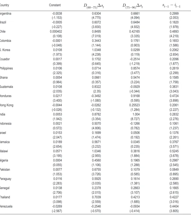
tructurAlchAngesGiven the belief that over time many countries have reduced their capital controls, one would expect a smaller correlation between saving and investment for more recent periods. To test the stability of the saving-investment relation, we estimate the following equation:
a (b1 1 b2 2) g( 1 1) e
t t t t t
i D D s s- i
-D = + + D + - + (5.1)
the literature indicates that there was a generalized trend towards greater capital mobility starting in the mid-1970s. Table 7 reports the results of the estimations. All the diagnostic tests are met.
table 7 – results of the estimation of the error correction model with structural changes
Country Constant
(60 75) t
D s
- D D(75 96)- Dst st-1-it-1
Argentina -0.0038 0.6304 0.6661 0.2999
(-1.153) (4.775) (4.094) (2.053)
Brazil -0.0005 0.6072 0.6484 0.1820
(-0.227) (3.830) (4.932) (1.978)
Chile 0.000402 0.8495 0.42165 0.4893
(0.108) (7.019) (3.335) (4.219)
Colombia -0.0001 0.3443 0.1761 0.1653
(-0.048) (1.144) (0.903) (1.586)
S. Korea 0.0108 1.0348 0.0299 0.2062
(1.973) (4.238) (0.119) (2.654)
Ecuador 0.0017 0.1702 -0.2514 0.2096
(0.399) (0.645) (-1.219) (1.877)
Philippines 0.0106 0.0714 0.8574 0.2619
(2.325) (0.316) (3.477) (2.299)
Ghana 0.0054 0.0661 0.5474 0.1585
(0.964) (0.357) (3.224) (1.758)
Guatemala 0.0108 0.8322 -0.0929 0.3831
(2.035) (2.35) (-0.344) (3.043)
Honduras 0.0217 -0.3492 0.9168 0.4724
(3.400) (-1.080) (5.595) (3.898)
Hong Kong -0.0044 -0.0262 0.25523 0.2061
(-0.026) (-0.132) (1.284) (2.227)
India 0.0053 0.8782 1.004 0.2832
(1.942) (3.354) (8.727) (2.276)
Indonesia 0.0021 0.5070 -0.1266 0.1061
(0.572) (4.806) (0.782) (1.237)
Israel 0.0153 0.1699 0.0506 0.1376
(2.047) (1.474) (0.192) (2.261)
Jamaica 0.0189 0.5671 0.0345 0.3767
(2.654) (3.232) (0.235) (3.571)
Malawi 0.0571 1.0346 0.3816 0.5245
(3.195) (2.955) (1.884) (3.678)
Nigeria 0.0004 0.4560 0.1965 0.2987
(0.055) (1.106) (1.288) (2.545)
Pakistan 0.0077 0.6755 0.1079 0.0849
(1.053) (3.726) (0.585) (0.895)
Paraguay 0.0116 0.5925 0.1614 0.2690
(2.283) (3.035) (1.381) (2.580)
Senegal 0.0138 0.2378 0.2663 0.1665
(2.706) (2.015) (3.107) (2.615)
Thailand 0.0177 0.7039 0.4213 0.4227
(3.098) (2.559) (1.685) (3.016)
Venezuela -0.0269 -0.2546 -0.0934 0.4404
(-2.567) (-0.570) (-0.414) (3.805)
Note: t statistic in parentheses.
change periods were tested. For Brazil, for example, we establish different regimes for 1960-1989 and 1990-96 (since economic opening really only got under way in 1990) but this hypothesis was also rejected. For all countries except Argentina, Brazil, Philippines, Ghana, Honduras, Hong Kong, India, Senegal and Venezuela, the saving-investment correlation is smaller in the second sub-interval. These changes are consistent with greater capital mobility.
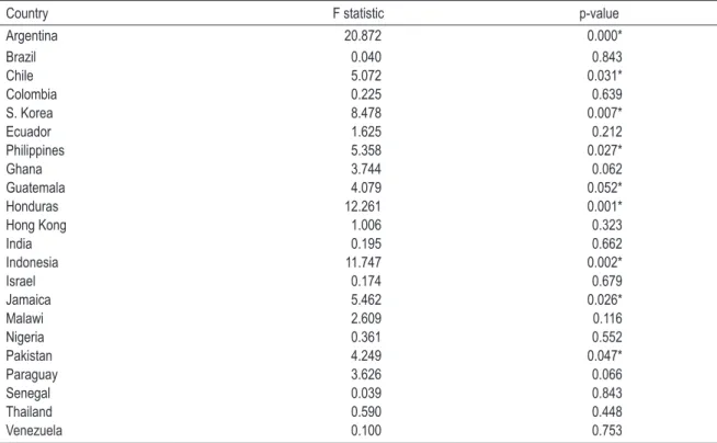
table 8 – tests of significance of structural changes
Country F statistic p-value
Argentina 20.872 0.000*
Brazil 0.040 0.843
Chile 5.072 0.031*
Colombia 0.225 0.639
S. Korea 8.478 0.007*
Ecuador 1.625 0.212
Philippines 5.358 0.027*
Ghana 3.744 0.062
Guatemala 4.079 0.052*
Honduras 12.261 0.001*
Hong Kong 1.006 0.323
India 0.195 0.662
Indonesia 11.747 0.002*
Israel 0.174 0.679
Jamaica 5.462 0.026*
Malawi 2.609 0.116
Nigeria 0.361 0.552
Pakistan 4.249 0.047*
Paraguay 3.626 0.066
Senegal 0.039 0.843
Thailand 0.590 0.448
Venezuela 0.100 0.753
Note: * means that the null hypothesis of constant coefficients is rejected at the 5% level of significance.
The error correction coefficients g do not substantially change in any of the countries. Again, the relevance of the intertemporal budget constraint is confirmed for Chile, Guatemala, Honduras, Jamaica, Malawi, Paraguay, Senegal, S. Korea, Thailand and Venezuela.
5 c
onclusionsThe purpose of this paper is to verify if the error-correction approach is the best alternative to asses capital mobility in developing countries, as argued by Jansen (1996) and Jansen and Schulze (1996) for developed countries. An error correction model is a synthesis of the other approaches in the literature and is the only one with theoretical backing. We also estimate the equation of Felds-tein and Horioka using the variables in levels and in first differences, to evaluate what type of bias these specifications imply.
mobility according to the criterion of Feldstein and Horioka. The specification in differences, on the other hand, does not result in bias. The same result is obtained by Jansen (1996) for developed countries. Jansen (1996) even establishes: “This is a reassuring idea when estimating saving-invest-ment correlations for developing countries, for which often only short time series are available and conse-quently the long-run relation cannot be reliably estimated. Forgetting about the long run and switching to a specification in differences seems then to be a reasonable strategy.” (p. 768). We believe, however, that perhaps it is not a question only of estimating the long-run relation reliably. The long-term co-efficient implies solvency. In this way, when g = 0 is not rejected, i.e., when saving and investment are not cointegrated, the intertemporal budget constraint is simply not met. Evidence in this sense, for developing countries, can be found in Sawada (1995). In this case, the correct specification is indeed the equation in differences.
We agree that in principle an error correction model should be a richer specification than those generally employed to assess capital mobility, but we disagree that it supplies more than one form of doing so, at least for developing countries. As seen before, cointegration between saving and investment or stationarity of the current account indicates solvency. If it is not possible to find evidence of cointegration, then this is indicative that the country does not meet its intertemporal budget constraint instead of evidence of capital mobility. As Jansen (1996) himself contradictorily states, “a lower g implies that a country is able to run for a longer time a deficit or surplus in excess of its long-run value. The intertemporal budget constraint is now less restrictive when a country tries to smooth its aggregate expenditure by borrowing or lending in the world capital market.”
A
ppendix– t
estsoFstAtionArityoFsAvingAndinvestmentThe results for the augmented Dickey-Fuller (ADF) and Phillips-Perron (PP) tests for invest-ment and saving (expressed as ratios of the product) are shown in Table A. 1.
table A.1 – unit root tests: saving and investment
Country Investment ADF
Saving ADF
Investment PP
Saving PP Argentina -2.059 -2.285 -2.228 -2.391 Brazil -2.592 -3.241 -2.752 -3.123 Chile -3.156 -1.928 -3.121 -2.623 Colombia -4.109* -3.243 -4.115* -2.691 S. Korea -2.957 -1.816 -3.057 -1.816 Ecuador -1.898 -2.027 -1.772 -2.084 Philippines -1.862 -1.864 -2.201 -1.652 Ghana -1.108 -1.866 -1.767 -3.937 Guatemala -2.247 -1.910 -2.158 -1.816 Honduras -1.260 -1.585 -2.159 -1.789 Hong Kong -1.497 -1.828 -2.070 -1.565 India -4.110* -3.196 -4.119* -3.187 Indonesia -1.300 -1.918 -2.361 -2.088 Israel -1.487 -2.304 -2.479 -2.391 Jamaica -1.668 -2.052 -1.543 -2.036 Malawi -2.479 -1.938 -2.349 -2.015 Nigeria -2.795 -2.112 -2.259 -2.171 Pakistan -3.400 -2.171 -3.489 -2.289 Paraguay -1.460 -3.017 -1.709 -2.979 Senegal -1.889 -2.272 -1.869 -2.121 Thailand -2.413 -2.149 -2.494 -2.011 Venezuela -2.484 -2.768 -2.549 -2.761
Notes: For the ADF statistic. the critical values at the 5% and 1% levels of significance are. respectively. –3.53 and –4.20. The regressions of the tests include a constant and trend. The number of lags is chosen based on the significance of the highest lag.
* means the null hypothesis is rejected at the 5% level.
r
eFerencesArgimón, I.; Roldán, J. M. Saving, investment and international capital mobility in EC countries. European Economic Review, 38, p. 59-67, January 1994.
Bagnai, A.; Manzocchi, S. Unit root tests of capital mobility in the less developed countries. Weltwirt-schaftliches archiv, v.132, n. 3, p. 545-557, 1996.
Baxter, M.; Crucini, M. J. Explaining saving-investment correlations. american Economic Review, v. 83, n. 3, p. 103-115, 1993.
Bayoumi, T. Saving-investment correlations: immobile capital, government policy, or endogenous behavior.
iMF Staff papers, 37, p. 360-387, June 1990.
Dickey, D. A.; Fuller, W. A. Likelihood ratio statistics for autoregressive time series with a unit root.
Dolado, J.; Jenkinson, T.; Sosvilla-Rovera, S. Cointegration and unit roots. Journal of Economic Surveys, 4, p. 249-273, 1990.
Dooley, M.; Frankel, J.; Mathieson, D. International capital mobility: what do saving-investment correla-tions tell us? iMF Staff papers, v. 34, n. 3, p. 503-530, 1987.
Engle, R. F.; Granger, C. W. J. Cointegration and error correction: representation, estimation, and testing.
Econometrica, 55, p. 251-276, 1987.
Feldstein, M. Domestic saving and international capital movements in the long run and in the short run.
European Economic Review, p. 129-151, 1983.
Feldstein, M.; Bacchetta, P. National saving and international investment. in: Bernheim, D.; Shoven, J. (eds.),
national saving and economic performance. Chicago: University of Chicago Press, 1991, p. 201-220. Feldstein, M.; Horioka, C. Domestic saving and international capital flows. Economic Journal, 90, p.
314-329, June 1980.
Finn, M. G. On saving and investment dynamics in a small open economy. Journal of international Eco-nomics, 28, p. 1-21, August 1980.
Frankel, J. International capital mobility and crowding-out in the U.S. economy: imperfect integration of financial markets or goods markets? in: Hafer, R. (ed.), How open is the u.S.economy? Lexington: Lexington Books for the Federal Reserve Bank of St. Louis, 1986, p. 33-67.
_______. Quantifying international capital mobility in the 1980s. in: Bernheim, D.; Shoven, J. (eds.),
national saving and economic performance. Chicago: Chicago University Press, 1991, p. 227-260. Granger, C. W. J.; Newbold, P. Spurious regression in econometrics. Journal ofEconometrics, v. 2, n. 2, p.
111-120, 1974.
Gundlach, E.; Sinn, E. Unit root tests of the current account balance: implications for international capital mobility. applied Economics, 24, p. 617-625, June 1992.
Haan, J.; Siermann, C. L. J. Saving, investment and capital mobility: a comment on Leachman (1991).
open Economies Review, 5, p. 5-17, 1994.
Harberger, A. C. Vignettes on the world capital market. american EconomicReview, v. 70, Papers and Proceedings, p. 331-337, 1980.
Jansen, W. J. Estimating saving-investment correlations: evidence for OECD countries based on an error correction model. Journal of international Money andFinance, 5, p. 749-781, 1996.
Jansen, W. J.; Schulze, G. G. Theory-based measurement of the saving-investment correlation with an application to Norway. Economic inquiry, v. XXXIV, p. 116-132, 1996.
Leachman, L. L. Saving, investment and capital mobility among OECD countries. open Economics Re-view, v. 2, Issue n. 2, p. 137-163, 1991.
Mamingi, N. Saving-investment correlations and capital mobility: the experience of developing countries.
Journal of policy Modeling, v. 19, n. 6, p. 605-626, 1997.
Miller, S. M. Are saving and investment cointegrated? Economics letters, 27, p. 31-34, 1988.
Montiel, P. Capital mobility in developing countries: some measurement issues and empirical estimates.
World Bank Economic Review, v. 8, n. 3, p. 311-350, 1997.
Murphy, R. G. Capital mobility and the relationship between saving and investment in OECD countries.
Journal of international Money and Finance, v. 3, p. 327-342, 1984.
_______. Productivity shocks, non-traded goods and optimal capital accumulation. European Economic Review, 30, p. 1081-1095, 1986.
Obstfeld, M.; Rogoff, R. The six major puzzles in international macroeconomics: is there a common cause?.
nBER Working paper 7777, 2000.
Phillips, P. C. B.; Hansen, B. E. Statistical inference in instrumental variables regression with I(1) processes.
Review of Economic Studies, v. 57, n. 1, p. 99-125, 1990.
Sawada, Y. Are heavily indebted countries solvent? Tests of intertemporal borrowing constraints. Journal of Development Economics, 45, p. 325-37, 1994.
Sinn, S. Saving-investment correlations and capital mobility: on the evidence from annual data. Economic Journal, 102, p. 1162-1170, September 1992.
Summers, L. H. Tax policy and competitiveness. in: Frenkel, Jacob A. (ed.), international aspects of fiscal policy, NBER Conference Report, Chicago: Chicago University Press, 1988, p. 349-375.
Tesar, L. Saving, investment, and international capital flows. Journal ofinternational Economics, 31, p. 55-78, 1991.
Tobin, J. Comment on “Domestic saving and international capital movements in the long run and short run, by M.S. Feldstein”. European Economic Review, 21, p. 53-156, 1983.