325
Abstract
Risk mapping processes in mine planning and ore recovery are constantly used in the mining industry to increase decision making certainty based on the available information. However, it is not possible to predict the risk behavior in all of the proj-ect’s boundary conditions and small variations in some of these conditions can cause a great impact on its inancial return. Among the countless uncertainties existing in a mining project (operational, costs, market change), many authors deine the geological uncertainty as the most critical one, capable of inluencing the success of the project. Measurement and evaluation of the geological uncertainty of a mine planning project is crucial because the calculated risk can be translated into a inancial risk of the proj-ect. This article presents a possible way to consider the geological uncertainty in the pit optimization step by using sequential Gaussian simulation. The results obtained from the case study on a copper deposit results in a simple procedure with signiicant increase in reliability for the project.
Keywords: risks, geological uncertainty, sequential Gaussian simulation, mine planning, pit optimization.
Rafael Alvarenga Souza
Mestrando
Universidade Federal de Ouro Preto - UFOP Escola de Minas
Departamento de Engenharia de Minas Ouro Preto – Minas Gerais - Brasil [email protected]
Ivo Eyer Cabral
Professor Adjunto
Universidade Federal de Ouro Preto - UFOP Escola de Minas
Departamento de Engenharia de Minas Ouro Preto – Minas Gerais - Brasil [email protected]
Incorporation of geological
uncertainty in pit optimization
with geostatistics simulation
Mining
Mineração
http://dx.doi.org/10.1590/0370-44672016700134
1. Introduction
The long term mine planning, also called strategic mine planning, corresponds to the process of deter-mining the best design and deter-mining scheduling, according to a previously established strategy. It is considered a key element for the success of a mining enterprise, since it controls the decision making concerning their conduction and development. One of the main challenges for the realization of a mining plan is to ensure that the developed plan is feasible and con-siders the geological and operational variabilities of the mine. Some plans, which are developed without knowl-edge of the possible variables, have a lower reliability that can result in intuitive decisions making, which is not always optimal, and may harm the achievement of the goals set for a long term.
Quantifying the uncertainties and risks involved in a planning project is a step that has a large inlu-ence on the pit limits and production scheduling. Impacts on the order of
millions of dollars can be provided by small variations and/or changes in project boundary conditions. Cost of capital, the market price of ore, at-tractive rates and operating costs are factors usually tested to analyze the feasibility of a project. However, even though these are considered by many authors as the main factor of failure in achieving the targets in mining industry, they are rarely considered as an uncertainty related to the geo-logical model.
Usually the estimate and dis-tribution of grades in a deposit are done by geostatistical and classical methods. Such methods result only in the estimated average values for the deposit, not being able to reproduce the actual spatial variability of data in situ. That variability is required in sensitivity engineering project analyses, since the variability of these contents imply variations in the inal value of the project, whose impact is generally unknown.
The stochastic conditional
simu-lation techniques allowed the real variability in situ to be evaluated. The methods of stochastic simulation were originally developed to correct the smoothing effect displayed on maps produced by kriging. Contrary to kriging, stochastic simulation meth-ods do not result in a single estimate of the map of the variable of interest. The geostatistical simulation methods aim is to reproduce the variability in situ, and the spatial continuity of the original data, by the generation of equiprobable scenarios, conditioned to data, reproducing the statistical characteristics of 1st and 2nd order of sample data. That way, the degree of uncertainty associated with the estimates can be evaluated.
2. Materials and methods
The kriging estimate is performed by minimizing the variance of the estimation error. Thus, it can be concluded that the estimate aims to offer the best possible estimate of an attribute without repro-ducing the original spatial heterogeneity of the data.
However, this minimization pro-vides lower variance than the original data. This reduction in variability is known as smoothing. As cited by Goo-vaerts (1997), all interpolation algorithms tend to smooth the spatial variability of the attribute. This effect is characterized by underestimation of high values and
overestimation of low values. Smoothing can be easily observed to comparing the histogram of a database with the result of their kriging estimation.
As shown by Olea (1999), the simulation was the solution adopted to solve the smoothing problem of kriging. But, according to the author, the gain in overall accuracy causes the reduction of local accuracy. In fact, the realizations of the simulation scenarios are not free from errors of reproducing reality and, on aver-age, the mistakes are higher than kriging. Therefore, simulations should not be thought of as a substitute method for
kriging, but as a variability and uncer-tainty veriication tool involved in kriging estimation, since kriging is still the best unbiased estimator.
Presented initially by Matheron (1973), the stochastic conditional simula-tion techniques allowed the variability and uncertainty involved in the estimation of mineral deposits to be quantitatively evaluated. Until that moment the kriging variance was the only existing way to evaluate the estimates. But Journel (1986) and, later, Brus and Gruijter (1993) began to question the use of this parameter as an estimative quality index.
2.1 Grade simulation
According to Deutsch and Journel (1992), the absence of an estimation er-ror component (R(x0)) provides
smooth-ing of krigsmooth-ing. The equation presented below shows that the real value of a particular attribute in a point x0 can be
written as the sum of its estimate with the estimated error.
Z ( x0 ) = Z* ( x0 )+ R ( x0 ) (1)
(2)
(3)
Thus, to have access to real vari-ability of the random function Z(x0), the random function R(x0) should be
simulated many times and added to the estimated value. Each ith simulated value in each of the simulation scenarios can be
written as the sum of the kriging value with the l-th realization of the random function R(x0).
Z l ( x
0 ) = Z* ( x0 )+ R l ( x0 )
Existing simulation methods seek to randomly determine the error component based on the known method of Monte Carlo. Thus, as the process is random, the realizations will be different, but honor-ing the sample histogram and the sample variogram model.
Histogram and variogram reproduc-tion is classiied as an overall accuracy. For the result of interpolation, the same sample statistic used in the estimation was maintained. Actually kriging, classiied as
a local precision method, does not produce the histogram and sample variogram, but shows a high correlation between estimated and used samples.
Among the many methods of sto-chastic simulation, the algorithms of se-quential simulation methods are the most used to reproduce the spatial distribution and uncertainty of different variables (Soares, 2001, p. 911). This greater uti-lization results from a greater simplicity of execution and eficiency, since other
methods, besides having a more complex use, may have limitations and/or problems with their results.
The multiplicand presented in Equa-tion 3 summarizes the theoretical basis of the sequential simulation methods, where each simulation generates a new point that is used to update the conditional cumula-tive distribution function. Thus, the condi-tional cumulative distribution function is always updated by a subsequent simulated value and the n sampling points.
F ( x
1,...,x
N;Z
1,...,Z
N|(n)) = F (x
1;Z
1|(n))
.F (x
2;Z
2|(n + 1))
. ...
.F (x
N-1;Z
N-1|(n + N - 2))
.F (x
N;Z
N|(n + N - 1))
=
∏
F (x
i;Z
i|(n + i - 1))
i = 1 N
The main and most common method used of sequential simulation on deposit modeling is the sequential Gaussian simulation method (SGS) because of its simplicity, lexibility and reasonable eficiency (Deutsch, 2002, p. 162). To use this method, one should
work with a normal distribution with null mean and unit variance, so data must receive prior to processing.
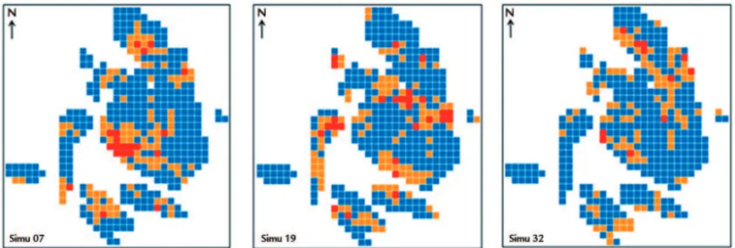
The block model of the de-posit, with a total of 33.807 blocks, was simulated in 50 scenarios using the sequential Gaussian simulation
327
Figure 1 Plan view of scenarios 7, 19 and 32 obtained from the simulation.
After performing the simula-tions, it is important to verify that the scenarios obtained as a result sat-isfactorily reproduce the distribution
of sample data and used variogram models. The 50 scenarios reproduce quite acceptably the sample distribu-tion (histograms) and spatial
continu-ity (variograms). The igure below is a variogram of all scenarios were well adherent to the variogram model in three main directions.
Figure 2 Validation of spatial continuity in the three main anisotropic directions.
2.2 Pit optimization
Obtaining the optimal pit was achieved by using the three dimensional optimization algorithm of
Lerchs-Grossman (1965), by NPV Scheduler
4 software. In the following table are shown the values and parameters used.
The sale price considered for copper was 2.06 $/lb (about 4,540 $/t).
Parameter Value Copper price 4,540.00 $/t Metallurgical recovery 83.70 %
Mining cost 3.50 $/tROM Processing cost 10.00 $/tROM
General angle 62°
Table 1 Technical and economic parameters
considered in the optimization step.
Figure 3 presents the mathematical pit obtained by optimizing the model estimated by ordinary kriging.
The optimization of simulated sce-narios follows the same premises adopted for the kriging model (Table 1). The only difference is that instead of using the esti-mated copper value by ordinary kriging as product, the value obtained by simulation in each scenario was used.
Due to the great demand of time
and the amount of information gener-ated, not all scenarios were optimized. In order to maintain the representation of all the simulations without the need to calculate the 50 pits, a criterion was adopted to select the simulations that participated in the study. In this criterion, the optimal extraction sequence (OES)
obtained by optimizing the kriging model was used to calculate the NPV of the 50 scenarios. Thus, the 50 NPV values found were ranked in increasing order and 11 scenarios were chosen to participate in the evaluation of the pit (Table 2), which divided the entire population into a range of 5 in 5 NPV values.
Scenario SIM Scenario SIM Scenario SIM 1 39 5 1 9 25 2 13 6 18 10 35 3 34 7 9 11 45 4 43 8 50
Table 2
Selected scenarios to calculate the final pit.
3. Results
The igure 4 shows the limits in the plant of 11 pits for the selected scenarios
compared to the pit limit of the kriging model (red line).
Figure 4
Comparison of the max
limit of the kriging model pit (in red) with the pits of simulated scenarios (in gray).
It can be seen that in certain regions the kriging model pit presents an opti-mistic behavior, being located externally to the simulated limits. While in other regions, the kriging pit has a more
conser-vative behavior in relation to the simula-tions. Such behavior can also be viewed in depth as shown in the following Figure 5. Areas with large variation limits in plant and depth can be used to deine
potential targets for additional drilling (Godoy, 2009). Thus, this great luctua-tion limits results from a high variability provided by the absence or small amount of information.
Figure 5
Vertical section in the direction
SW-NE presenting the difference in depth of the kriging model pit (in red) with the pits of simulated scenarios (in gray).
In the following Figure 6 is shown the amount of ore contained in each of
the incremental pits obtained by opti-mizing the kriging model and selected
simulated scenarios.
Figure 6
329
By analyzing the previous igure, it is easy to see that the kriging model pit stands out from the others by having a greater amount of ore and, consequently, a lower strip ratio. Such disparity was provided by the known smoothing effect of ordinary kriging, where low values were overestimated and high values were underestimated.
By performing smoothing, the krig-ing brought a certain amount of material that should be below the cutoff grade for higher grade values, transforming part of the low grade material to ore. This ex-plains the greater amount of ore presented in the graphic of the previous igure.
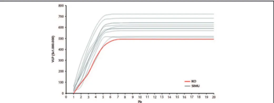
The lack of low values reproduc-tion for the estimate was evidenced by
the contained ore graphic, but the lack of high values reproduction can easily be seen in the following igure 7, where the absence of very high grade blocks (responsible for a large increase in the value of the NPV) provides a low NPV for the pit of the model estimated by ordinary kriging compared to the pits of simulated models.
Figure 7 NPV comparison of kriging model pit with pits simulated.
4. Conclusion
Approaching the geological uncer-tainty with the application of geostatis-tical simulation techniques proved to be an essential and indispensable tool in the evaluation of long term mine planning projects. Although it is not
widely used, quantifying the geological uncertainty with the use of geostatisti-cal simulation can considerably reduce the possible risks associated with some project factors.
As the shown in the results, when
only considering the model estimated by ordinary kriging as absolute truth, there is a great risk that the estimates of net present value (NPV), quantity of ore and strip ratio of the selected inal pit do not relect the reality.
References
BRUS, D. J., GRUIJITER, J. J. Does kriging really give unbiased and minimum variance predictions of spatial means? Journal of Soil Science, v.44, n.4, 1993. DEUTSCH, C. V., JOURNEL, A. G. Geostatistical software library and user’s
guide - GSLIB. Oxford University Press, 1992. 340 p.
DEUTSCH, C. V. Geoestatistical reservoir modeling. New York: Oxford University Press, 2002. 376 p.
GODOY, M. A risk analysis based framework for strategic mine planning and design - method and application. Orebody Modelling and Strategic Mine Planning, Perth, WA: 2009. 7p.
GOOVAERTS, P. Geostatistics for natural resources evaluation. New York: Oxford University Press, 1997. 483 p.
JOURNEL, A. G. Constrained interpolation and qualitative information – the soft kriging approach. Math. Geol., v. 18, n°. 3, p. 269-286, 1986.
LERCHS, H., GROSSMANN, I. F. Optimum design of open pit mines. CIM Bulletin, v. 58, p. 47-54, 1965. (January).
MATHERON, G. The intrinsic random functions and their applications: Advances in Applied Probability. v. 5, p. 439-468, 1973.
OLEA, R. A. Geostatistics for engineers and Earth scientists. Boston: Kluwer Acade-mic Publishers, 1999. 303 p.
SOARES, A. Direct sequencial simulation and cosimulation. Math. Geol., v. 33, p. 911-926, 2001.