Abstract
To measure the aerodynamic and hydrodynamic forces and mo-ments acting on scaled models in water and wind tunnel tests, multi-component strain gauge force and moment balance are usu-ally used. Their performance and accuracy largely depends on the rig and calibration method, including the load table (design matrix) and analysis of experimental data. In this article, for the calibration of a six-component balance, a calibration procedure using the Box-Behnken design (BBD) of experiments was developed. In the sug-gested design matrix, in addition to all possible combinations of the two-component load of the six component load (Test vectors with two active factors), the pure loads (test vectors with one active fac-tor) are also used. The implementation of the design matrixwas done using a calibration rig, which has the ability to perform formal experimental design techniques completely. The obtained experi-mental data were fitted with second-order equations using regres-sion analysis. The statistical significance of independent variables and interactions was tested using the analysis of variance (ANOVA) with 95% confidence (α = 0.05). The results of residuals indicate that the suggested model sufficiently predicts the responses as a function of input factors. The comparison between the Modified Box-Behnken design (MBBD) and BBD calibrations indicates that the MBBD method estimates the data more accurate. The results show that the MBBD method is the most appropriate method com-pared to the existing methods for calibrating balance in this paper.
Keywords
Calibration experiment, strain gauge balance, statistical analysis, Box– Behnken experimental design, Response surface methodology (RSM)
Development and Evaluation of Calibration Procedure for a
Force-Moment Balance Using Design of Experiments
1 INTRODUCTION
To measure the aerodynamic and hydrodynamic forces and moments acting on scaled models in water and wind tunnel tests, multi-component strain gauge balances are usually used. Considering the re-lationship between forces and the output signal of the balance and using calibration models, direct
N.M. Nouri a* Karim Mostafapour b
a,b School of Mechanical Engineering,
Iran University of Science and Technol-ogy, Tehran, Iran
* Corresponding author.
Tel: +982177240540x2982; fax: +982177240488.
E-mail address: mnouri@ iust.ac.ir.
http://dx.doi.org/10.1590/1679-78252307
Latin American Journal of Solids and Structures 13 (2016) 119-135
measurement of forces and moments acting on the model in water and the wind tunnel is provided. Calibration of a balance means identifying the equations which can be used to calculate the loads acting on the model based on the output signals. These equations are called the equations of balance interference effects. Regression is a method for modeling and analyzing the numerical data. The data include some values for the dependent variable and six independent variables. The purpose of the regression analysis is to express the dependent variable as a function of the independent variables and the error coefficients (a kind of a random variable). The accuracy of determining the mathematical model and the duration of the calibration experiment largely depends on the design matrix and the analysis of the recorded data. In the general case, the details of the design matrix are largely under the control of the researcher. In fact, the number of rows depends on the number of experiments which is desirable for the researcher. The number of columns depends on the selected mathematical model. The value of each term of the design matrix is determined by the load schedule. The experi-mental runs (load tables) should be selected based on the appropriate criteria to predict a multinomial model.
Since 1940, several load tables have been employed in the calibration process of the multi-com-ponent balance. Given its simplicity and ease of understanding, the traditional method of one factor at the time table (OFAT) is widely accepted as a method for balance engineers. This method has been used in Langley Research Center (LaRC) since 1940 (Hansen, 1956). The calibration method of the OFAT is started by the first-order calibration of pure loads and followed by second-order calibra-tion with all 15 combinacalibra-tions of the two components. First-order and second-order calibracalibra-tion include 253 and 481 experimental runs, respectively. The loading is done manually on these systems. The disadvantages of these systems are the complex loading process, the sensitivity to the experimental conditions, and the need for six to eight weeks for loading (Ferris, 1996).
To reduce the duration of the manual methods of the experiment, the automated balance cali-bration systems have been developed (Ewald, 2000). The main advantages of these systems are the prevention of the potential loss of the operator power, reduction of the load time, and application of the combined loads. The disadvantages of this scheme are the mechanical complexity of the system, inaccuracy in setting the direction of load toward the balance, and increase in systematic errors.
Latin American Journal of Solids and Structures 13 (2016) 119-135 The most common designs, i.e. the central composite design (CCD) and the Box-Behnken design (BBD), of the principal response surface methodology have been widely used in various experiments. In 2001, for the first time, NASA employed a modified central composite design (MCCD) for balance calibration (Parker et al., 2001). This design is known as the single vector system (SVS) calibration method. In this system, the automated calibration routine is coupled with a MCCD. In SVS, balance calibration is done based on a single vector. In this system, the force and moment vectors are perpen-dicular to each other on each loading point. In recent years, several studies have been conducted based on SVS. Deloach and Philipsen (2007) applied the Stepwise Regression Analysis on data ob-tained from SVS. They compared the obob-tained results with OFAT. Bergman and Philipsen (2010) compared the Load Tables using OFAT and SVS to estimate the coefficients of calibration. These reviews show the high accuracy and execution time reduction of calibration in SVS compared to OFAT. In SVS, in addition to loads, Lynn et al. (2011) mentioned the pressure and temperature of wind tunnel as influencing factors in the calibration equations. Connecting error due to the complexity of the system and inaccuracy in setting the direction of the loading toward the balance increases the systematic error in the SVS method. Given the complexity of the component combinations in the SVS design matrix test vectors, the performance of experimental runs using the manual calibration rig is time consuming and often inaccessible. To calibrate a six-component balance by the calibration rig, Simpson et al. (2008) used the second-order Box–Behnken design. In this method, for each test vector, two active factors are employed. The primary constraint on calibration equipment limits the simultaneous application of pitch moment and yaw. To resolve this problem, the desired points have been revised in the test matrix based on rig limitations. To evaluate the performance of the BBD, Simpson and his colleagues compared the obtained calibration results with the SVS method. In the BBD method, there is a reduced test time and improved precision. In the calibration test using BBD, Landman et al. (2013) considered temperature as an influencing factor in the calibration mathematical model. In the BBD method, to estimate the coefficients of the first- and second-order calibration of the mathematical model, each test vector is considered as the combination of the two component load. The combination loads used in BBD can include the nonlinear interaction in the calibration rig. Part of this nonlinear interaction can appear in the calibration coefficients of force and moment balance and decrease the regression model accuracy to estimate the forces and moments of voltages.
In this article, to decrease the effect of nonlinear interaction of the calibration rig on the calibra-tion coefficients of the six-component balance, the design matrix has been developed as Modified Box-Behnken design (MBBD). In this method, in addition to using two factors in the test vectors of the load table, test vectors with an active factor are added to the load table to decrease the effect of the nonlinear interaction of the calibration rig. The calibration tests were carried out using a six-DOF calibration rig which has the ability to apply a different combination of six component loads simul-taneously and independently. In this article, the obtained results using the statistical analysis for calibration models of BBD and MBBD were compared.
2 THE CONCEPTS OF CALIBRATION EQUATIONS
second-Latin American Journal of Solids and Structures 13 (2016) 119-135
order polynomial. In this model, the output voltage of each strain gauge bridge is considered as a dependent variable and function of the loads on the balance. This is the most common model which is used for the strain gauge balances’ calibration. The general form of a complete second-order poly-nomial is equal to (Tropea et al., 2007):
6 6 6
i
1 1
i j
R
A
j ijk jj j
k j k
F
B F F
(1)During load calibration, F is known, and the signals, Ri, are measured. In Equation 1, error terms
are shown as
.A
ij is the indicator of 36 first-order coefficients andB
ijk is the indicator of 126second-order coefficients. Six members of
A
ij with i=j are the direct sensitivity for 6 loads. Theinteraction terms are represented by the off-diagonal elements of the matrix. In equation 1, the com-ponents of
A
ij with i j indicate the linear interactions. A first-order interaction is the linear effectof a load component on the measuring point output of other components. For example, the strain created in the strain gauges installation location, which is used for measuring the normal force, can be caused by normal force and other components. Other reasons for first-order interactions include strain gauge misalignment and improper connection in the assembly process. In equation 1, the non-linear coefficients are indicated by
B
ijk . The case of j k is the sensitivity second-order ofinterac-tions and indicates the nonlinearity of the sensitivity second-order interacinterac-tions. The case of j k
indicates the second-order product interactions. Second-order interactions are caused by the change in the elastic mode of different parts which are quadratic and nonlinear. Equation (1) can be written in the vector form of Equation (2):
y X (2)
y
is the response measuring vector, is the coefficients vector,X
is the design matrix, and
contains the error terms. The design matrix plays a key role in determining the quality and the cost of the calibration tests. The impact of the design matrix on quality can be investigated through a covariance matrix which indicates the variance in the estimation of regression coefficients and the predicted response by the model. The covariance matrix (C) is a square matrix (p×p). It is obtained through the following equation.1 2
C(X'X) σ (3)
Where,
X
is the design matrix and2Latin American Journal of Solids and Structures 13 (2016) 119-135 coefficients can be estimated simply by optimizing the design matrix in different ways. Similarly, variance of balance response estimated values strongly depend on the design matrix. There are certain terms of the design matrix which affect the efficiency and quality of results modeling. These terms are controllable. The design matrix is determined based on load schedule. Experimental runs (design matrix) should be selected based on appropriate criteria to predict a polynomial model. These criteria are more common in the RSM method (Myers et al., 2009). The response Surface Methodology (RSM) is an experimental technique invented to find the optimal response within the specified ranges of the factors. These designs are capable of fitting a second-order prediction equation for the response. The optimality of a design depends on the statistical model. It is assessed with respect to a statistical criterion, which is related to the variance-matrix of the estimator.The six most popular criteria are (Montgomery, 2011):
1.Power: Power is the probability of detecting an effect, like the normal force input or the interaction of the normal force input and the yaw moment input, of a specific size that is relative to the standard deviation of the system.
2.The scaled D-optimality criterion: The D-optimality criterion minimizes the variance associ-ated with the coefficients in the model. Scaling allows comparison of designs with a different number of runs. Relatively low values of the scaled D-optimality criterion are preferred and indicate a small volume of the joint confidence interval of the model coefficients.
3.A-optimal designs: An A-optimal design is one that minimizes the individual average vari-ances of the model coefficients. Lower values of the average prediction variance will result in smaller confidence intervals for predictions from regression models.
4.G-efficiency: The G-efficiency is a simple measure of average prediction variance as a percent-age of the maximum prediction variance. If possible, one should try to get a G efficiency of at least 50%.
5.V-optimal designs: V-optimality minimizes the average prediction variance over a specified set of design points. Lower values of the maximum prediction variance will result in smaller confidence intervals for predictions from regression models.
6.Variance Inflation Factor (VIF): In multiple regression, the variance inflation factor (VIF) is used as an indicator of multicollinearity (correlation between predictors). VIF is always greater than or equal to 1. A common rule of thumb is that if VIF>5 then multicollinearity is high. To design an appropriate calibration matrix, the above standards should not be considered, but the limitations of the calibration rig must be understood.
3 DESIGN MATRIX OF EXPERIMENTAL RUNS
3.1Box-Behnken Designs (BBD)
Latin American Journal of Solids and Structures 13 (2016) 119-135
factors, corresponding to the coded values. Such designs are, in this way, more efficient and economical then their corresponding 3k designs, mainly regarding a large number of variables. Another advantage
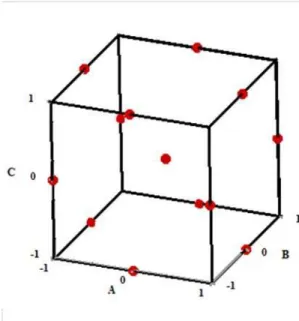
of the BBD is that it does not contain combinations for which all factors are simultaneously at their highest or lowest levels. So these designs are useful in avoiding experiments performed under extreme conditions, for whichunsatisfactory results might occur. Box and Behnken (1960) suggested how to select points from the three-level factorial arrangement, which allows the efficient estimation of the first- and second-order coefficients of the mathematical model. In this study, a six-component balance was calibrated for use in testing the models of closed water-tunnel circuits. The six factors chosen for the study are designated as NF, AF, SF, PM, RM, and YM,and the predicted response is designated as V. Details of load size,lower limit, and upper limit of the factor are givenin Table 1. Each of the independent variables was consecutively coded at three levels: −1, 0, and 1. In the BBD design for the calibration balance, the design of the experiment vector includes all probable structures (60 com-binations of the two active factors) of the two active factors.
Figure 1: The experimental runs of a three-factor BBD.
S.no Factor Input Level, Uncoded [coded]
Low Medium High
1 AF(N) 0[-1] 20 [0] 40 [1]
2 NF (N) -20 [-1] 0 [0] 20 [1]
3 SF (N) -20 [-1] 0 [0] 20 [1]
4 RM (N.m) -1 [-1] 0 [0] 1 [1]
5 PM(N.m) -1 [-1] 0 [0] 1 [1]
6 YM(N.m) -1 [-1] 0 [0] 1 [1]
Latin American Journal of Solids and Structures 13 (2016) 119-135
3.2 Modified Box-Behnken Designs (MBBD)
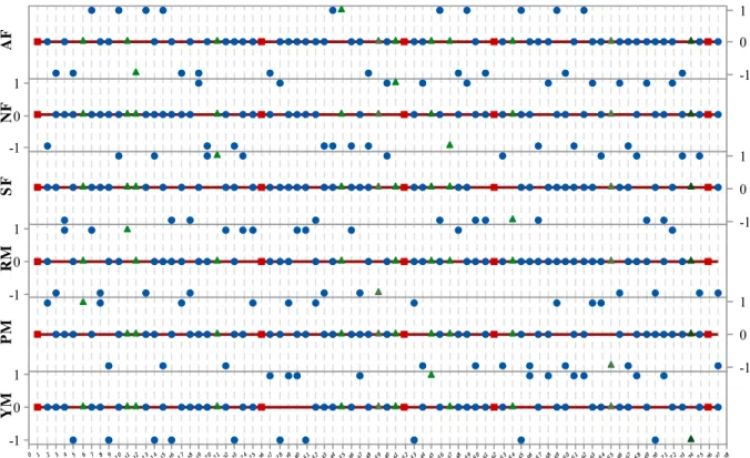
The Modified Box-Behnken designs (MBBD) test vectors are plotted in Figure 2. The vertical axis represents the coded values and the horizontal axis represents the run order in the calibration test. To increase the statistical independence of the calibration data, test vectors in the design matrix are randomized. In the load table, each test vector contains 6 factors. Three levels of -1, 0, and 1 are considered for each factor. The total runs in the calibration test contain 77 test vectors. In this design, the experiment vectors contain all first-order and second-order combinations.
Figure 2: Matrix Plot of NF, AF,SF, PM, RM and YM vs Run Order.
On 60 test vectors which are shown in the plots with circles, two factors are used as active loads. These points include all possible combinations of the two-component loads plus the six-component load located at the corner of the plots. These test points can provide a favorable condition to estimate the non-linear effects caused by balance deviation, which appears in second-order coefficients of the calibration equation. In 12 vectors, there are some tests in the middle of the edges. There are indica-tion by the triangle symbol. These tests are added to the BBD method. In these tests, one factor is used as an active load. In calibration tests, one active factorare known as pure load acting on balance. Pure loads can be used to estimate the first-order coefficients (sensitivity and linear responses).
The overall design contains 5 center points to estimate the pure error.Theseare indicated by a square symbol. The goodness of experiment design can be stated in terms of quantity. By assuming
1 0 -1 1 0 -1 1 0 -1 1 0 -1 1 0 -1 78 77 76 75 74 73 72 71 70 69 68 67 66 65 64 63 62 61 60 59 58 57 56 55 54 53 52 51 50 49 48 47 46 45 44 43 42 41 40 39 38 37 36 35 34 33 32 31 30 29 28 27 26 25 24 23 22 21 20 19 18 17 16 15 14 13 12 11 10 9 8 7 6 5 4 3 2 1 0 1 0 -1 AF NF SF RM PM
Run O rde r
Latin American Journal of Solids and Structures 13 (2016) 119-135
5% α-level for effects, statistical measures were calculated for BBD and MBBD. Values of power, G-efficiency, scaled D-optimality criterion, A-optimal designs, A-optimal designs, and VIF for both methods are shown in Table 2. The power of the MBBD main effects is equal to 99.6 percent, which is greater than the power of the BBD main effects (99.2%). Setting the calibration rig’s first-order interaction interference with the balance calibration model in an independent orientation and, accord-ing to the accuracy requirements, may decrease the influence of calibration rig’s nonlinear interaction on the calibration coefficients of the six-component balance.
BBD (two-active factor) MBBD
criterion
99.2 % 99.6 %
Power at 5% alpha level for effect of 2Std. Dev Main effect
99.9 % 99.9 %
Pure quadratics
49.5 % 50.0 %
Two factor interactions
8.211 9.166
Scaled D-optimality
0.431 0.364
Average Prediction Variance (A-optimal)
0.450 0.427
Maximum Prediction Variance at a design point (V-optimal)
95.7% 85.0%
G-efficiency
1.47 1.41
VIF(multi-collineary)
Table 2: Comparison of statistical criterions for calibration models of MBBD and BBD.
4 CALIBRATION EQUIPMENT
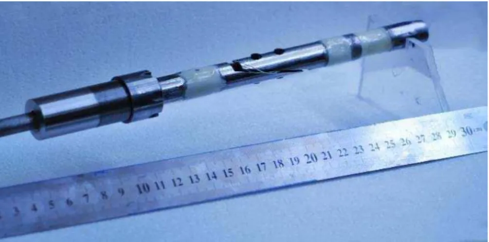
The balance considered in this study is a six-component balance which has the capability of measuring the forces NF, AF, and SF and the moments PM, RM, and YM directly and simultaneously. The balance is designed in such a way to measure the forces and moments acting on the model which are parallel to the coordinates and are attached to the axis of the model. The flexural elements and strain gauge are used to design the balance. Each component of the force or moment is on a special elastic element based on the created strain. The balance is shown in Figure 3.
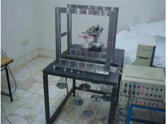
Latin American Journal of Solids and Structures 13 (2016) 119-135 To run the tests of multi-component force-moment balance calibration, a six-DOF calibration system was designed. The design of this rig is based on the formal experimental design techniques, the use of the gravity direction for balance loading and the simplicity of positioning and aligning of balance compared to the gravity direction. The calibration rig has the ability to apply a different combination of component loads simultaneously and independently to calibrate the internal six-component balances. In this rig, the balance is put into a sleeve, and the balance end is fixed to the sting. The loads is applied to the balance using the frame parallel to the axes attached to the balance. Pulleys located on the shaft can be placed in different positions parallel to the sleeve grooves. They can make the load application possible in different situations. Balance loading can be conducted using the standard calibration weights of the F2 series ((OIML standard weight),(OIML R 111, 2004)). The direction of the load application and the direction of the axes attached to the balance should be parallel to each other. To parallelize and to set the balance position, an angle adjustment and a six-degree of freedom system is designed. Using this system, the balance can be put in a favorite position such that the yaw and pitch angle are perpendicular and parallel to the gravity direction. To detect the amount of balance deviation from the gravity device, the balance mounted on the sleeve is used. The direction and position of the balance are set based on the laser alignment line (with an uncer-tainty of 0.1mm / 1m) which acts upon gravitational principles. Therefore, the balance direction and position can be set based on the axis device. Figure 4 shows the calibration rig during the six-compo-nent balance calibration tests. During the calibration test, the loads were act on the balance using deadweights. The measuring section outputs are recorded using a data acquisition system. Through 12 available scales and weights, the combination of independent loads is provided.
Latin American Journal of Solids and Structures 13 (2016) 119-135
5 STATISTICAL ANALYSIS OF EXPERIMENTAL DATA
In the calibration tests, loads were recorded as independent variables, and signals were recorded as dependent variables. The regression model predicted gauge output as a function of load. First, the outputs of the measuring sections were recorded as functions of the calibration load based on the loading table. The calibration coefficients were determined according to the recorded data and statis-tical analyses. Next, the regression coefficients were converted to the reduced matrix coefficients, and the loads were iteratively and inversely estimated from the outputs of the measuring sections. Vari-ance was analyzed to ensure that requirements were met. Information related to the analysis of vari-ance (ANOVA) for the calculation of the regression model are presented in Table 3.
Source DF SS MSE
R
S S
Lack of fit(LOF) n-(p+m)
t t t
y y b X y
t t t
PE
y y b X y
RSS
LOF
LOF SS df
Pure error(PE) m
21 1 j n m ij j j i
RSS pure error
y y
PE PE SS df ) , , (b0 b1 bpSS
) (b0
SS 1
n
y
2) | , ,
(b1 b 1 b0
SS P p - 1 btXtYny2
2
1
t t
b X Y ny
p
Table 3: Analysis of variance table for the least squares fit,p: number of parameters in the model; n: total number of observations runs; m: number of center points.
The unexplained variance (SSR) was divided into two individual components, i.e. lack of fit
(SSLOF) and pure error (SSPE). SSLOF relates to the capability of the mathematical model in receiving
the responses of the electrical signals as a function of the independent variables. SSPEis a function of
Latin American Journal of Solids and Structures 13 (2016) 119-135 number of observations. R-sq (adj) is calculated as 1 minus the ratio of the mean square error (MSE) to the mean square total (MS Total). R-sq (pred) is calculated by systematically removing each observation from the data set, estimating the regression equation, and determining how well the model predicts the removed observation.
6 CALIBRATION RESULTS
For the calibration balance, the BBD was found to be more suitable than other tested designs (Simp-son et al., 2008; Landman et al., 2013;Simpson, J. et al., 20050). In this section, calibration results for
the MBBD experimental runs are presented. The obtained results are compared with the BBD.
6.1 Determination of the Regression Coefficient and Statistical Evaluation
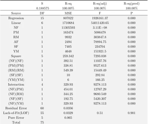
By applying a multiple regression analysis on the design matrix and the responses, the regression coefficient in coded form was established. The significance of the independent variables and their interactions were tested by means of the analysis of variance (ANOVA). For example,table (4) in-cludes a part of the ANOVA data for normal force.
S R-sq R-sq(adj) R-sq(pred)
0.188575 100.00% 100.00% 100.00%
Source DF MSE F P
Regression 15 807022 1926161.37 0.000
Linear 6 1710684 54011420.65 0.000
NF 1 11305593 3.11E+08 0.000
PM 1 163474 5086478 0.000
RM 1 9932 303847.8 0.000
AF 1 2494 78894.75 0.000
SF 1 7405 234704 0.000
YM 1 4648 151921.5 0.000
Square 5 259.342 7293.038 0.000
(NF)(NF) 1 392.51 11037.76 0.000
(PM)(PM) 1 338.81 9527.613 0.000
(RM)(RM) 1 549.39 15449.49 0.000
(SF)(SF) 1 10 292.84 0.000
(YM)(YM) 1 6 166.25 0.000
Interaction 4 329.93 9278.113 0.000
(NF)(PM) 1 454.01 12767.29 0.000
(NF)(RM) 1 344.25 9680.549 0.000
(NF)(SF) 1 192.75 5420.307 0.000
(NF)(YM) 1 329.93 9278.113 0.000
Residual Error 60 0.0356
Lack-of-Fit(LOF) 55 0.0329 0.51 0.901
Pure Error 5 0.065
Total 75
Latin American Journal of Solids and Structures 13 (2016) 119-135
An alpha (
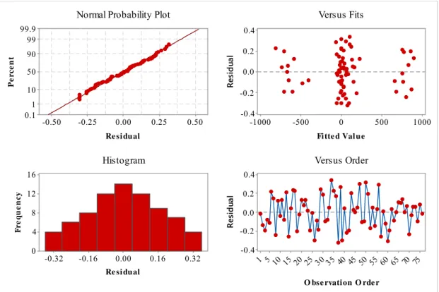
) level of 0.05 was used to determine the statistical significance in all analyses. This indicates that the model terms are significant at 95% of the probability level. All coefficients that were below this probability were removed; the reduced model is shown in Table 4. The p values for all the coefficients of the reduced model were lower than 0.05. This means that the terms in the regression model have a significant correlation with the response variable. The F-value of 0.51 with p-value of 0. 901 gives no indications for a more complex model. A very high value of the correlation coefficient (R-sq = 100.00%) exhibited an excellent correlation between the experimental and pre-dicted response values. The value of the adjusted determination coefficient (R-sq (adj) = 100.00%) is very high and confirmed that the model was highly significant. The R-sq a value was found to be very close to the R-sq (adj). These results indicate that additional terms do not improve the model more than is expected by chance. The value of the predicted determination coefficient (R-sq (pred) = 100.00%) is close to the R-sq. This result indicates that the model does not suffer from overfitting and does not predict new observations as well as it fits the existing data. The repeatability of the measurement environment can readily be determined from the MSE of the pure error part. The maximum standard deviation of pure error was 0.033% of the maximum response. The values for the standard deviation of pure error showed that the repeatability of the calibration was less than the residual error. Thus, thederived mathematical model used to predict a response produce a result inside the accuracyrequirement.We made the assumptions that all of the error terms are identically and independently normally distributed with a mean of 0 and common variance sigma–square. Examining the residual plots shown in Figure 5 helps to determine whether the ordinary least squares assumptions are being met.
Figure 5: Residual Plots for Normal Force 0.50 0.25 0.00 -0.25 -0.50 99.9 99 90 50 10 1 0.1
Re si dual
P e rce n t 1000 500 0 -500 -1000 0.4 0.2 0.0 -0.2 -0.4
Fitte d Value
Res id u a l 0.32 0.16 0.00 -0.16 -0.32 16 12 8 4 0
Re si dual
F r e q ue nc y 75 70 65 60 55 50 45 40 3 5 3 0 25 20 15 10 5 1 0.4 0.2 0.0 -0.2 -0.4
O bse rvation O rde r
Res
id
u
a
l
Normal Probability Plot Versus Fits
Latin American Journal of Solids and Structures 13 (2016) 119-135 The points on the normal probability plot form a nearly linear pattern, which indicates that the normal distribution is a good model for this data set. The points on the residuals versus fitted values plot appear to be randomly scattered around zero, so assuming that the error terms have a mean of zero is reasonable. The vertical width of the scatter doesn't appear to increase or decrease across the fitted values, so we can assume that the variance in the error terms is constant. The histogram plot shows that a normal distribution of variation results in a specific bell-shaped curve, with the highest point in the middle near zero and smoothly curving symmetrical slopes on both sides of center. These features provide strong indications of the proper distributional model for the data. The Residual vs. Order of the Data plot was used to check the drift of the variance during the experimental process, when data are time-ordered. The residuals are randomly distributed around zero, which means that there is no drift in the process.
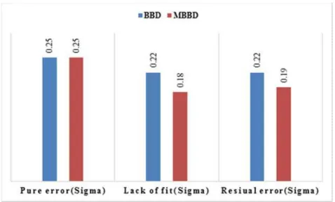
Unexplained variance obtained by the two methods of BBD and MBBD on response for normal force section is presented in Figure 6. The comparison between the two methods shows the same pure error (the repeatability) anddifferentLOF. The residual due to the lack of fit in the MBBD method is less than the lack of fit of BBD. During the calibration test, setting the direction of the balance toward the gravity direction is directly carried out by the calibration rig. Therefore, the difference of the obtained LOF cannot be due to the interference of the linear deviation of the calibration rig toward the balance. This difference may be due to the calibration rig nonlinear systemic effects inter-ference with the second-order interaction of the balance. Using the tests with an active factor (pure loads acting on the balance) in MBBD, the calibration rig’s nonlinear systemic effects on the balance calibration model will be reduced.
Figure 6: Unexplained variance for normal force section.
6.2 The Accuracy of Calibration Methods
Latin American Journal of Solids and Structures 13 (2016) 119-135
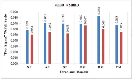
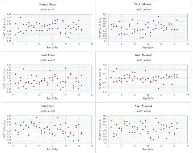
voltage is considered as a response. In an iterative and reverse process, the voltage loads have been calculated using the estimated coefficients. In Figure 7, the comparison of two sigma values for the residuals errors are provided for calibration models. These values are scaled according to the maxi-mum load. They are expressed as a percentage of the full scale. These accuracies are estimated using the residuals for all components. The comparison between the accuracy of the BBD and MBBD methods indicates that the MBBD method estimates the data more accurately. In the MBBD method, the test vectors with an active factor are added to the load table to decrease the effect of nonlinear interaction of the calibration rig. The accuracy increase is due to the pure loads fitted to linear coefficients of the MBBD method.
Figure 7: The comparison of the residuals errors for calibration models of MBBD and BBD.
6.3 The Investigation of Confirmation Points
Latin American Journal of Solids and Structures 13 (2016) 119-135 Figure 8: The confirmation point residuals for forces and moments of calibration models.
Latin American Journal of Solids and Structures 13 (2016) 119-135
7 CONCLUSIONS AND SUMMARY
In this article, to decrease the effect of nonlinear interaction of the calibration rig on the calibration coefficients of the six-component balance, the design matrix has been developed as the Modified Box-Behnken design (MBBD). The adequacy of the estimated mathematical model has been checked by various descriptive statistics. The F-value of 0.51 with p-value of 0. 901 gives no indications for a more complex model. Predicted values obtained using the quadratic model equation were in very goodagreement with the observed values (R-sq = 100.00%, R-sq (adj) = 100.00%, R-sq (pred) = 100.00%).The value of the adjusted determination coefficient (R-sq (adj) = 100.00%) is close to the R-sq. This result indicates that the model does not over-fit and does not predict new observations as well as it fits the existing data. The maximum standard deviation of pure error was 0.033% of the maximum response. The values for the standard deviation of pure error showed that the repeatability of the calibration was less than the residual error. Thus, the derived mathematical model used to predict a responseproduce a result inside the accuracy requirement. The validationresults of the data show no systematic difference between confirmation and model residuals. A comparison between the BBD and MBBD calibrations shows that the MBBD calibration tends to be most accurate.The com-parison between BBD and MBBD indicates that given the application of pure loads corresponding to linear coefficientsin MBBDdecreases the effectiveness of the calibration rig’s nonlinear interaction on a six-component balance calibration coefficients. The calibration statistical results show that using the load tables of MBBD, in calibration experimental runs, is more suitable for a six-component balance in this paper, compared to other methods.
References
Bergman, R., Philipsen, I., (2010). An Experimental Comparison of Different Load Tables for Balance Calibration. 27th AIAA Aerodynamic Measurement Technology and Ground Testing Conference, AIAA 2010-4544.
Box, G. E. P. and Behnken, D. W., (1960). Some New Three Level Designs for the Study of Quantitative Variables. Technometrics 4: 455 – 475.
Box, G. E. P. and Wilson, K.B., (1951). On the Experimental Attainment of Optimum Conditions (with discussion). Journal of the Royal Statistical Society Series B13 (1):1–45.
Deloach, R. and Philipsen, I., (2007). Stepwise Regression Analysis of MDOE Balance Calibration Data Acquired at DNW. AIAA-2007-0144, 45th AIAA Aerospace Sciences Meeting and Exhibit, Reno, Nevada, January 8-10.
Ewald, F.R, (2000). Multi-component force balances for conventional and cryogenic wind tunnels. Meas. Sci. Tech-nol.11 R81-R94. 20th Conference, Albuquerque, NM, June 15-18.
Ferris, A. T., (1996).Strain Gauge Balance Calibrationand Data Reduction at NASA Langley ResearchCenter. Paper DR-2, First International Symposiumon Strain Gauge Balances. October.
Fisher, R. A, (1925)." Statistical Methods for Research Workers" Oliver & boynd.
Hansen, R.M., (1956). Evaluation and Calibration of Wire-Strain-Gage Wind-Tunnel Balances under Load. NACA Langley Aeronautical Laboratory.
Latin American Journal of Solids and Structures 13 (2016) 119-135
Lynn, K. C., Commo, S. A., Johnson, T.H., Parker, P. A., (2011). Thermal and Pressure Characterization of a Wind Tunnel Force Balance using the Single Vector System. AIAA 2011-950.
Montgomery, D.C., (2011). Design and Analysis of Experiments. 8th ed., John Wiley and Sons Inc., NY.
Myers, R. H., Montgomery, D. C., Anderson-Cook, C. M., (2009). Response Surface Methodology. 3rd ed., John Wiley and Sons Inc., NY.
OIML R 111(2004). Weights of classes E1, E2, F1, F2, M1, M1–2, M2, M2–3 and M3.
Parker, P.A., Morton, M., Draper, N., Line, W., (2001) .A Single-Vector Force Calibration Method Featuring the Modern Design of Experiments. AIAA 2001-0170, 39th Aerospace Sciences Meeting and Exhibit, Reno, Nevada. Simpson, J. et al., (2008). Adapting Second-Order Response Surface Designs to Specific Needs. Quality and Reliability Engineering International24(3): 331-349.
Simpson, J. et al., (2005). Calibrating Large Capacity Aerodynamic Force Balances using Response Surface Methods. AIAA 2005-7601, December.