Alexandro Garro Brito* Institute of Aeronautics and Space
São José dos Campos – Brazil [email protected]
*author for correspondence
Computation of multiple limit
cycles in nonlinear control
systems – a describing function
approach
Abstract: Limit cycles play an important role in nonlinear systems, provided that many control loops with common nonlinearities like relay, hysteresis, and saturation can present them. Thus, a proper description of this nonlinear phenomenon is highly desirable. A strategy for the linearized analysis is the describing function method, which is a frequency domain approach that allows the limit cycle prediction and stability analysis. Some
papers had discussed the method for the simpliied analysis; however,
they are concentrated in the prediction of only one limit cycle even for systems with multiple conditions. This paper proposes a systematic way of multiple limit cycle determination, as well as the stability analysis of each one. All theoretical/computational issues involved in the approach are also discussed.
Keywords: Limit cycle, Multimodal optimization, Describing functions.
INTRODUCTION
Nonlinear behavior is common in aerospace systems, where many kinds of nonlinearities can produce limit cycles or other phenomena that can affect the system overall behavior. In Dotson, Baker and Sako (2002), the limit cycle induction due to aerodynamic forces over launcher fairings and aircraft wings was discussed. Leite Filho and Bueno (2003) presented the analysis of self-sustained oscillations in actuator systems of a launch vehicle. Furthermore, Newman (1995) and Stout and Snell (2000) studied the presence of this nonlinear behavior in spacecrafts and launchers propulsion systems.
Due to the limit cycle phenomenon importance in several systems, a systematic approach to predict its amplitude and frequency is necessary, and many methods based on an analytical analysis have been proposed. For predator-prey systems, a proper formulation can be derived to predict limit cycles, as seen in the works of Freedman (1990), Hofbauer and So (1994); however, it cannot be directly extended to other dynamic systems. In Nayfeh and Mook (1979), two important general methods are presented: the Lindstedt-Poincar’e and the Multiple Scales, both of them based on a linearization through power-series expansion and algebraic manipulations that can become hard in some cases.
In spite of extremely useful, the methods mentioned above consider that the nonlinear part can be written as a power-series, which implies that the nonlinearity must be differentiable. Obviously, this is not ever the case, mainly in nonlinear control loops where several discontinuous elements can be present. Then, alternative methods, in which the differentiability is not a requirement, should be adopted. One of the most reliable methodologies is the harmonic balance, where the input-output relation is expressed through the Fourier series (Slotine and Li, 1991). This strategy is much less restrictive than a power-series and can be applied to a wider class of nonlinear systems, including the discontinuous ones. If one is interested in an approximate result, the analysis of the
Fourier-series fundamental used to be suficient, leading to the
describing function method, which is a generalization of linear frequency response for nonlinear systems (Gelb and Velde, 1968; Gibson, 1964; Slotine and Li, 1991), and it provides a graphical way to determine the limit cycle existence as well as its amplitude and frequency. In Kienitz (2005) and Somieski (2001),
the describing function method was modiied so that
the existence of limit cycles is related to a functional minimization. Thus, one can obtain the amplitude and frequency of the limit cycle by a unimodal optimization of that functional.
However, even this method cannot be directly applied if one is interested in obtaining information about multiple limit cycles of a dynamic system. This paper presents a methodology to compute all limit cycle conditions of nonlinear systems. It is based on a multimodal optimization
algorithm, which is able to ind all the global minima of
a cost-function related to the limit cycle occurrence. In spite of other methods like multimodal genetic algorithms that can lose some global minima depending on the cost function topology (Darwen and Yao, 1996), the proposed procedure was developed to guarantee that all minima are reached, even those in complex topological regions like sharp attraction basins.
The theory associated with limit cycle calculation is presented, including the describing function concept and the stability analysis. In this paper, this strategy is expanded to permit the computation of multiple limit cycle conditions through the multimodal optimization algorithm presented herein. To test the methodology, some common nonlinearities are associated with simple linear systems, in order that multiple limit cycle conditions appear. Then, the algorithm is used to calculate the amplitude and frequency of the limit cycles and their stability.
LIMIT CYCLE DETERMINATION
Methods for quantitative analysis of limit cycle are very useful in a lot of practical applications. Different approaches were developed along time, each one with
their beneits and disadvantages. Some of them will be
further discussed.
Power-series expansion
Take into consideration a nonlinear system governed by equations, having the following form (Eq. 1):
x f x( R0)"0 (1)
where f is a nonlinear function. Assuming that this function can be expanded by Taylor series, it can be rewritten as in Eq. 2:
x nx n
N n "
"
¨
F 10 (2)
where (Eq. 3):
Fn nn R n
f t " y
y
1
0
! ( ).
(3)
There are several ways to obtain an approximate solution of Eq. 2, most of them based on a perturbation analysis around the initial condition u0. The Lindstedt-Poincar’e Method writes the solution as polynomial expansions over two independent variables related to the oscillations
amplitude and frequency (Nayfeh and Mook, 1979). This strategy permits that the nonlinear differential equation is converted to a number of algebraic equations; the precision of the approximate solution is strongly related to the polynomial order. This method gives uniformly valid approximations; however, the algebraic manipulation becomes complex for relatively low orders. Another technique is the method of multiple scales, in which the polynomial expansion is a function of multiple independent variables instead of only one. Though more involved, it is also able to treat the damped systems (Nayfeh and Mook, 1979).
The power-series approaches – mainly the method of multiple scales – have been successfully applied in many systems where limit cycles are expected to appear. In Li et al. (2008), the bifurcations of multiple limit cycles for a rotoractive magnetic bearings were considered and an approximate solution was obtained through the mentioned method. The same ideas are also applied in Mendelowitz, Verdugo and Rand (2009), in which the limit cycles for coupled oscillators were studied. Yu and Corless (2009) performs the limit cycle computation of the Hilbert’s 16th problem – a complex system where the analysis through the multiple scales requires intensive symbolic computations.
Besides very useful to analyze a huge class of nonlinear systems, the power-series methods present some drawbacks. First of all, they assume that the nonlinear function (Eq. 2) is analytic around u0, which implies that one can differentiate f (u) as much as necessary. This is true for several systems, such as the one expressed as a polynomial function (Li et al., 2008; Yu and Corless, 2009). However, it is not always true for nonlinear control loops. In these cases, the presence of nonlinear elements like saturation, backlash, and other equipments that exhibit
a discontinuous proile can become the method of multiple
scales impossible to apply. Moreover, the use of symbolic manipulation softwares like Maple and Mathematica is essential for multiple limit cycle computation, and the computational effort can also be relatively high even for simple nonlinear control loops. Another important disadvantage is that one cannot obtain any information about the unstable limit-cycles through these methods. It is important to notice that information about unstable oscillations are very useful in control analysis.
Harmonic balance and describing function
Slotine and Li, 1991), the harmonic balance method seemed to be more appropriate (Nayfeh and Mook, 1979). It is based on the nonlinear function expansion through Fourier series, much less restrictive than Taylor’s. Collecting the harmonics of f (u) properly, the user is also able to rewrite the nonlinear equation as set in algebraic equations.
The describing function analysis is a special case of the harmonic balance, in which only the fundamental contribution of the Fourier series is used (Siljak, 1969). The system can be seen in Fig. 1a, with a sinusoidal input of amplitude A and frequency ω. The output can be expanded by Fourier series as in Eq. 4,
y t a an n t b n t n
n
( )" cos( ) sin( ).
" h
¨
0 1
2 \ \ (4)
with coeficients given by Eq. 5 to 7:
a0" 1 y t d t
µ
U U \
U
( ) ( ) (5)
an " 1
µ
y t n t d tU U \ \
U
( ) cos( ) ( ) (6)
bn " y t n t d t
µ
1
U U \ \
U
( ) sin( ) ( ) (7)
If the nonlinear element satisies some conditions so that
its output can be properly approximated by its fundamental Fourier expansion (Slotine and Li, 1991), then (Eq. 8):
y t( )~a1cos(\t)b1sin(\t)" M \ ^t " \ ^
M t Mej t
( ) sin( ) { ( )
~ \ \ " \ ^ " \ ^ }} (8)
where, ℑ represents the imaginary part of a complex
number. The describing function is deined as (Eq. 9):
N A Me Ae
j t
j t
( , )
( )
\ " \ ^\
(9)
which is dependent of both input frequency ω and amplitude A. Let’s consider the Fig. 1b, where G(jω) represents the linear part of the system, while N(A, ω) is the describing function of the nonlinear element. According to Nyquist criterion, self-sustained oscillation occurs in this loop if and only if (Eq. 10):
G j N A G j
N A
( ) ( , ) )
( , )
\ \ \
\ " 1
¡
" 1(10)
Applying Nyquist stability criterion over (Eq. 10), one can notice that each intersection between the curves G(j ω) and
−1/N(A, ω) in the Nyquist complex plane corresponds to
a limit cycle. The limit cycle’s frequency and amplitude are given by the values ω = ωLC and A = ALC, where the curves intercept themselves, respectively.
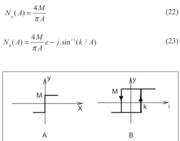
Figure 1: Diagrams for nonlinear analysis.
Asin(\t)
N(A,\) N(A,\) G(j,\) y(t) +
A B
The Eigenvalue Method (Somieski, 2001) is an approach that uses a persistent eigenvalue analysis of the nonlinear
closed loop to ind the limit cycle. To systematize the limit
cycle analysis, let’s rewrite the system represented in Fig.
1 as a set of irst order nonlinear equations (Eq. 11):
x" Fx f x x( , ) (11)
where, x is a state vector, F is a system matrix representing the linear part and f is a matrix with the nonlinearities. The nonlinear matrix f is linearized by the describing function concept yet discussed, producing (Eq. 12):
f x x( , )
¡
N A( , ) ;\ x N A( , )\ "N jN (12)where, N(A, ω) is the describing function of Nℜand Nℑ are the real and imaginary parts of N(A, ω), respectively. Applying this formulation to Eq. 11 and by using the Laplace notation, one can obtain the linearized matrix for the closed loop given by (Eq. 13):
"© «ª
¹
ȼ
I N F N
\ 1
( ) (13)
which produces the eigenvalue problem (Eq. 14):
(sI)x"0 (14)
Note that Nℑ = 0 and
F
=F+Nℜ for static nonlinearities.
Using this representation for the linearized nonlinear system, a limit cycle occurs if a purely complex eigenvalue pair exists for some A ≡ ALC and ω ≡ ωLC. The computation approach used in the eigenvalue method is a rigorous sweep over the A×ω space, evaluating and analyzing the eigenvalues until a purely complex pair occurs. In Somieski (2001), a frequency iteration procedure is presented for
a ine calculation when a frequency dependence over
F
=exists. Obviously, this is not a proper way for systematic limit cycle search, because even regions without limit cycles must be researched, becoming an eigenvalue-based
Another way to limit cycle computation was presented in Kienitz (2005), where the optimization procedure is based on singular values evaluation. The process is possible due to the following condition:
Theorem 1 (Singular Value Condition): The complex matrix
F
=(A,ω) has a purely imaginary eigenvalue withmagnitude ωLC, if and only if the matrix 15:
"" j I\ ( , )A\ (15)
is singular at ω = ωLC and A=ALC (Kienitz, 2005).
S
is singular if and only if its minimum singular value, denotedby σ (S), is null at ω = ωLC. Then, a limit cycle exists at ω
= ωLC and A = ALC if the optimization problem (Eq. 16)
(ALC,\LC)"arg min ( )X " (16)
has a solution and σ (
S
(ALC, ωLC)) ≡ 0.
The singular value method presents an important advantage: the singular values computation is easier and faster than the eigenvalues one, increasing the
computational eficiency. Then, this is the preferable
method for limit cycle computation.
MULTIPLE LIMIT CYCLE SEARCH
There are some procedures to compute multiple limit cycle in the literature, however they are based on the analytical analysis of the nonlinear differential equation (Hofbauer and So, 1994; Li et al., 2008; Mendelowitz et al., 2009; Yu and Corless, 2009), which cannot be suitable for nonlinear control systems so that many of their nonlinearities are discontinuous. The describing function is useful in these cases, but the optimization procedure above (Eq. 16) must
be modiied, since it is a unimodal optimization process
intended to search only one limit cycle in a search space. The objective of this section is to present an optimization algorithm able to extend the singular value method above to the multiple limit cycle computation.
A irst attempt would be trying to use classical multimodal
optimization procedures within the cost-function (Eq. 16), but most of them are constructed to obtain all the minima in situations not much restrictive, which the attraction basins have similar aspect and are not very sharp. These issues were well discussed in Darwen and Yao (1996) study, the most common multimodal genetic methods were there discussed and compared. In their conclusions, one can note that a purely evolutionary multimodal method can lose some of the sharper attraction basins unless a high population size is used. Obviously, this is unacceptable in a multiple limit cycle search because the algorithm
can become excessively slow without guaranteeing that every minimum will be found. Other methods based on the simulated annealing technique suffer from the same problems (Gibson, 1964).
This paper proposes a mixed populational-deterministic
optimization method able to ind multiple minima in
a safer fashion. It is based on an initial population that evolves along the attraction basins through a gradient-like procedure, and converge to the global minima gradually.
During the process, many “ineficient” points (with high
cost-function or close to another better-ranking point) are progressively discarded, increasing the computational speed. As it will be discussed herein, the number of parameters to be set is not as high as other methods, and their tuning is much more intuitive.
Mixed populational-deterministic multimodal algorithm
Let’s consider J(x) a cost-function to be minimized. Therefore, the mixed populational-deterministic multimodal algorithm (MPDMA) procedure is as it can be seen in Fig. 2. Firstly, the search region should be spread out with N initial points (PopInitial), so that all possible attraction basins can be properly researched. The amount of points will depend on the search region size and the number of global minima. As an initial attempt, the user can set this value bigger than 100 times of the expected minima number. If the region size is very large (A, ω ≥
50), we recommend a ratio bigger than 200.
The next step consists in a Gradient-like procedure, where each point walks under the functional surface following the opposite direction of the local gradient vector. This is computed through an eight-sided regular polygon with a small radius Rpoly around each point, as shown in Fig. 3a; the base point xk is replaced by the vertex x1 since that it has the lowest value for the functional f(x). The Gradient-like procedure is applied over the prior population Pop(k
− 1) to obtain the current population Pop(k), and over that to obtain the next one Pop(k + 1); as stressed below, this will be necessary to update Rpoly that should be initially chosen around 1% of the search region range.
During the population evaluation, some points can be far from a possible minima. Because of this, a selection procedure is necessary to discard such points so that only well-ranked points remain in the optimization. This selection is performed in two steps: i) points outside of the search region are automatically discarded; ii) after the
This is achieved throwing out all points inside a disc in the A×ω space, except the best one. The selection is
performed as stated: irstly, all points are sorted according
to their cost-function values in descending order. The
irst point is selected and a R-ray disc centered in this
point is evaluated; all other points inside this disc are discarded. Then, the next non-discarded point is selected and the procedure is repeated. The strategy is repeated until only non-neighbors remain. Figure 3b summarizes this selection level – points inside the gray discs will be discarded except the black ones, which are the best solutions in their respective disc. The radius R should chosen between 2 and 10% of the maximum range of
A and ω (region search). The user should avoid bigger values, for the algorithm can merge two near attraction basins, losing one of them.
After some iterations, the population evolution over the minima stops since that the polygon radius Rpoly is not ever
suficient to provide more precise convergence. The result
is that the global minima begin to be surrounded, but the
points are not able to reach them and this is relected by
the fact that the prior population (Pop(k-1)) become equal to the future one (Pop(k+1)). When this occurs, Rpoly should be
decreased by a rate, so that a iner evolution is possible and
the prior population (to be used in the next iteration) is taken as the mean between Pop(k) and Pop(k+1). Values for rate
around 2/3 provided good results. The algorithm is inished
when Rpoly is less than the precision deined by the user.
NONLINEAR CONTROL SYSTEMS – MPDMA APPLICATION TO REAL EXAMPLES
Many relatively simple nonlinear control systems can exhibit multiple limit cycles. In the describing function context, this means that all interceptions between G(jω) and
−1/N(A, ω) represent limit cycles which the stability will determine the attraction or repulsion of near trajectories in the phase plane. Then, the existence of multiple limit cycles is expected in every system where these multiple
intersections occur. Notice that ininite combinations
between a linear and a nonlinear model can provide the conditions above and the number of examples is really huge. Only to demonstrate some situations where multiple limit cycles occur, let us suppose the following examples.
Liénard system
A Liérnard system can be represented by the set of differential equations (Eq. 17):
x y F x y x
" " ¯ ° ±²
¿ À Á²
( ) (17)
In this paper, we use F(x) as Eq. 18:
F x( )"0 8. xG x( ) (18)
where G(x) = −4/3 x3 + 0.32 x5. In Giacomini and Neukirch (1997), an analytic method to determine the number of limit cycles of Eq. 18, and an approximate solution were presented. It showed that this system has one stable limit-cycle and another unstable. Obviously, one could use a power-series expansion method to obtain the approximate solution, since that G(x) is already expanded. However, the
Figure 2: MPDMA lowchart.
method of multiple scales becomes tedious to apply and a symbolic software is necessary. Moreover, none information about the unstable limit-cycle would be obtained.
By using the method of describing function over G(x), one can apply the MPDMA procedure to obtain information about both limit-cycles. Initially, the describing function of G(x) can be obtained through the Fourier expansion, according to Eq. 4-8, producing Eq. 19:
NG x( )( )A " A2( .0 2A21) (19)
Substituting Eq. 19 into 18, we have the describing function matrix: " ¬ ® ¼ ¾ ½
0 8 1
1 0
. NG x( )( )A
½½ (20)
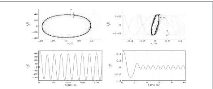
Figure 4 shows the contour plot for the cost (Eq. 16) (in right). There are two attraction basins related to the limit cycles. On the left, the system simulation and the approximate solutions are presented. To compute these approximations for both limit cycles, the MPDMA procedure was applied and the results are shown in Table 1. Notice that the amplitude and frequency of the limit cycles are in absolute accordance to Giacomini and Neukirch (1997).
The nonlinear matrix F can be obtained straightforwardly through Eq. 21 and 22 or 23 in Fig.1b, leading to:
"
0 1. 0.9 0.9487 0 0 0 --0.1 0.9487 0 0
0 0 -0.1 1 0
0 0 0 -10 1 0 0 0 0 10
0 0 0 0 1 ¬ ® ¼ ¾ ½ ½ ½ ½ ½ ½ ¬ ® ¼ ¾ ½ ½½ ½ ½ ½ ½ ¬ ® . ( ). . . N A 0 9487 0 9487 1 0 0 ¼¼ ¾ ½ ½ ½ ½ ½ ½ T (24)
where N(·)(A) is each of the describing functions above.
Figure 5: Some relay elements: (a) relay; (b) hysteresis.
M M
y y
X k
A B
Relay control system
The relay control is widely applied; however, it can
present self-sustained oscillations that inluence over the
system behavior, and they should be analyzed. In some cases, unstable and multiple limit cycles can be present and it is important to have consistent approaches to study each of them.
Relay elements are discontinuous by deinition so that a
linearization procedure based upon analytical expansions becomes hard to apply. To avoid this drawback, the describing function method has been used to analyze control loops with these elements. In Fig. 5, some relay elements widely used in control applications are shown. To exemplify situations where multiple limit cycles can occur, let us consider the control loop in Fig. 1b, where the linear part can be represented by the transfer function:
G s s
s s ( ) ( ) ( . ) ( ) " 3 1
0 1 10
2
3 2 (21)
According to Gibson (1964), the describing function of each relay element above is given by Eq. 22 and 23:
N A M
A a( )"
"
4
U
U
(22)
N A M
Ae j k A
b( ) .sin ( / )
"
" 4 1 U
U (23)
Figure 4: Liénard system. The contour plot for the cost function (Equation 16) is in the left. In the right, the system simulation and the describing function approximate solutions (continuous lines) are presented. The internal continuous line represents the unstable limit cycle.
Limit Cycle Amplitude Frequency
Unstable 0.9996 ± 0.0007 1.0000 ± 0.0004 Stable 2.0000 ± 0.0004 0.9998 ± 0.0008
Table 1: MPDMA application to the Liénard System (Eq. 18); 100 optimizations were performed with search region range equal to 4. The other adopted parameters were
Figure 6: Stable limit cycles for the relay controller (Eq. 22) with M = 20 and the linear part given by Eq. 21. Top: the phase plane; bottom: the output time evolution.
Figure 7: Stable limit cycles for the hysteresis controller (Eq. 22) with M = 3.125, k = 0.02 and the linear part given by Eq. 21. Top: the phase plane; bottom: the output time evolution.
The relay, as the hysteresis case, has three limit cycles, two of them stable. Their time response is presented in Figs. 6 and 7.
To obtain the whole information about these nonlinear systems, the MPDMA procedure was applied. The results are summarized in Table 2. Notice that the results are in perfect accordance with the simulations in Figs. 6 and 7.
CONCLUSIONS
This paper presented a new systematic approach intended to compute the multiple limit cycle conditions through the describing function method. Presently, this classical methodology for self-sustained oscillations analysis was applied to describe only one limit cycle, but many systems
Relay element
Limit
cycle Amplitude Frequency
Na(A) S 0.058 ± 0.003 8.1 ± 0.2 U 2.33 ± 0.03 0.808 ± 0.006
S 37 ± 2 0.261 ± 0.005
Nb(A) S 0.048 ± 0.006 2.7 ± 0.2 U 0.24 ± 0.04 1.0 ± 0.2 S 6.3 ± 0.1 0.253 ± 0.02
Table 2: MPDMA applied to the relay controllers; 100 optimizations were performed with search region range equal to 40. The other adopted parameters were N = 250, NSel2 = 50, NSel1 = 10, Rpoly(0) = 1%, R = 8%
can present multiple conditions that conduct to oscillatory trajectories. Herein, the describing function criterion was discussed for multiple limit cycle existence and numerical analysis.
The multiple limit cycle computation is based on an optimization algorithm that guides an initial population to the optimal points. In spite of its population character, the method is quite different of multimodal genetic algorithms: the points evolve following a deterministic Gradient-like procedure and the selection approach is different, as discussed during the text.
The optimization algorithm was very robust and precise in all practical cases presented in the paper, and the computational cost was acceptable. Furthermore, it was able to catch all global minima even in very sharp
attraction basins. This characteristic, which is dificult to
achieve with other methods, is important to the multiple limit cycle detection.
The main disadvantages of the proposed methodology
are concerned to problems with very lat attraction
basins, or which the topology presents non-differentiable regions because the Gradient-like procedure assumes differentiability condition. Despite many theoretical and practical problems have non-differentiabilities only in regions with high cost-function values, other optimization methods should be studied in cases which these issues become crucial to obtain a proper limit cycle description.
REFERENCES
Darwen, P., Yao, X., 1996, “Every niching method has its
niche: itness sharing and implicit sharing compared”, Lecture
Notes in Computer Science, Vol. 1141, pp. 398-407.
Dotson, K.W., Baker, R.L. and Sako, B.H., 2002, “Limit-cycle oscillation induced by nonlinear aerodynamic
forces”, American Institute of Aeronautics and
Astronautics Journal, Vol. 40, No. 11, pp. 2197-2205.
Freedman, H. I., 1990, “A model of predator-prey dynamics
as modiied by the action of a parasite”, Mathematical
Biosciences, Vol. 99, No. 2, pp. 143-155.
Gelb, A., Velde, W., 1968, “Multiple-input describing
functions and nonlinear system design”, McGraw Hill,
New York, USA..
Giacomini, H., Neukirch, S., 1997, “Number of limit
cycles of the li´enard equation”, Physical Review E, Vol.
56, No. 4, pp. 3809-3813.
Gibson, J.E., 1964, “Nonlinear automatic control”,
McGraw Hill, New York, USA.
Hofbauer, J., So, J.W., 1994, “Multiple limit cycle for
three dimensional lotka-volterra equations”, Applied
Mathmatics Letters, Vol. 7, No. 6, pp. 65-70.
Kienitz, K., 2005, “On the implementation of the eigenvalue
method for limit cycle determination in nonlinear systems”,
Nonlinear Systems, Vol, 45, pp. 25-30.
Leite Filho, W., Bueno, M., 2003, “Analysis of
limit-cycle phenomenon caused by actuator’s nonlinearity”,
In Proceedings of the 20th Inter. Conf. Appl. Simul. and Modeling.
Li, J., Tian, Y., Zhang, W. and Miao, S., 2008, “Bifurcation of multiple limit cycles for a rotor-active magnetic bearings
system with time-varying stiffness”, International Journal
of Bifurcation and Chaos, Vol. 18, No. 3, pp. 755-778.
Mendelowitz, L., Verdugo, A. and Rand, R., 2009, “Dynamics of three coupled limit cycle oscillators with
application to artiicial intelligence”, Communications in
Nonlinear Science and Numerical Simulation, Vol. 14, No. 1, pp. 270-283.
Nayfeh, A.H.,Mook, D., 1979, “Nonlinear oscillations”,
Wiley, New York, USA.
Newman, B., 1995, “Dynamics and control of limit
cycling motions in boosting rockets”, Journal of Guidance,
Control and Dynamics, Vol. 18, No. 2, pp. 280-286.
Siljak, D., 1969, “Nonlinear systems – the parameter
analysis and design”, John Willey & Sons, New York,
USA.
Slotine, J.J., Li, W., 1991, “Applied nonlinear control”,
Prentice Hall, New York, USA.
Somieski, G., 2001, “An eigenvalue method for calculation
of stability and limit cycles in nonlinear systems”,
Nonlinear Dynamics, Vol. 26, pp. 3-22.
Stout, P., Snell, S., 2000, “Multiple on-off valve control
for a launch vehicle tank pressurization system”, Journal
of Guidance, Control and Dynamics, Vol. 23, No. 4, pp. 611-619.
Yu, P., Corless, R., 2009, “Symbolic computation of
limit cycles associated with hilbert’s 16th problem”,