ISSN 0104-6632 Printed in Brazil
www.abeq.org.br/bjche
Vol. 25, No. 04, pp. 813 - 821, October - December, 2008
Brazilian Journal
of Chemical
Engineering
A SOFTWARE FOR PARAMETER ESTIMATION
IN DYNAMIC MODELS
M. Yuceer
1*, I. Atasoy
2and R. Berber
21
Inonu University Faculty of Engineering Department of Chemical Engineering, Phone: +(90) 422 3410010, Ex: 4753, Fax: +(90) 422 3410046, 44280, Malatya, Turkey.
E-mail: [email protected]
2
Ankara University Faculty of Engineering, Department of Chemical Engineering, 06100, Ankara, Turkey.
E-mail: [email protected], E-mail: [email protected]
(Received: April 1, 2007 ; Accepted: May 5, 2008)
Abstract - A common problem in dynamic systems is to determine parameters in an equation used to represent experimental data. The goal is to determine the values of model parameters that provide the best fit to measured data, generally based on some type of least squares or maximum likelihood criterion. In the most general case, this requires the solution of a nonlinear and frequently non-convex optimization problem. Some of the available software lack in generality, while others do not provide ease of use. A user-interactive parameter estimation software was needed for identifying kinetic parameters. In this work we developed an integration based optimization approach to provide a solution to such problems. For easy implementation of the technique, a parameter estimation software (PARES) has been developed in MATLAB environment. When tested with extensive example problems from literature, the suggested approach is proven to provide good agreement between predicted and observed data within relatively less computing time and iterations.
Keywords:Parameter estimation; Dynamic simulation.
INTRODUCTION
Parameter estimation is a common problem in many areas of process modeling, both in ‘on-line’ applications such as real time optimization and in ‘off-line’ applications such as the modeling of reaction kinetics and phase equilibrium. The goal is to determine the values of model parameters that provide the best fit to measured data, generally based on some type of least squares or maximum likelihood criterion. The estimation of parameters in kinetic expressions from time series data is essential for the design, optimization, and control of many chemical systems. The models that describe the kinetics take the form of a set of differential algebraic equations. The statistics and formulation of this parameter estimation problem are well studied (Bard, 1974). In the most general case, this requires
the solution of a nonlinear and frequently non-convex optimization problem, which can be approached by dynamic programming (with substantial programming effort and computer time), Pontryagin’s maximum principle (that requires solution of adjoint vector whose initial values creating extra problems) or nonlinear programming techniques.
state variables) map with respect to the parameters. This method requires calculation of the sensitivities by integrating an extra set of differential equations at the expense of computation time. Esposito and Floudas (2000) provided an underestimating formulation for this method. In their work, two deterministic global optimization methods are introduced for the parameter estimation of models that involve differential algebraic systems. Parameter estimation in dynamic models has been studied and discussed by several workers (Tjoa and Biegler,1991, Albuquerque and Biegler, 1996; Arora and Biegler, 2001, Neumann et al., 2007)
Vassiliadis et al.’s (1994) control vector parameterization method in the same direction, although carries out the optimization in the space of decision variables, uses Lagrange polynomials for expressing control variables and again converts the problem into a finite dimensional NLP with added complexity in the algorithm.
From the perspective of existing software for dynamic model calibration, there are a number of programs available commercially, some of them being accessible via Internet. However, most of them cannot fit some needs of the studied system satisfactorily even though they excel in other fields. For example the OPTKIN software supports large scale sets of equations with many parameters, but little customizability of these equations is allowed (Huybrechts and Van Assche, 1998). Therefore it is quite an efficient tool for the treatment of large sets of first order reactions (e.g. various radical mechanisms) but it does not allow application on some more complicated models. There are also limited possibilities for more detailed analysis of reliability and significance of parameters. The only generally applicable types of programs are the academic and semi-academic ones (Stewart et. al., 1992) but they are supplied as source code and provide poor user interface and require programming skills. Although ERA software package developed by Zamostny and Belohlav (1999) is a useful regression analysis tool, its input data matrix is limited to 20 independent variables and 20 responses, with up to 256 experimental points in each response and the number of model parameters is restricted to 15. Therefore, the floor seems to be open for further developments.
In this work, we have developed an integration based efficient algorithm, and a software for implementation, for parameter estimation in dynamic models without requiring calculation of sensitivity equations. The results obtained for some problems from the literature are compared, and its effectiveness is demonstrated.
OPTIMIZATION OVERVIEW
Optimization techniques are used to find a set of design parameters, x= {x
1, x2, x3,….., xn}, that can in
some way be defined as optimal. The objective function, f(x), to be minimized or maximized, may be subject to constraints in the form of equality constraints, inequality constraints and parameter bounds.
General problem may be defined as
( )
n
x
min f x
∈ ℜ ,
[
]
T n 1 2 n
x= x , x ,", x ∈ℜ (1)
subject to the constraints
( )
( )
j
j
l u
g x 0 j 1, 2,..., m
h x 0 j 1, 2, ..., r
x x x
= =
≤ =
≤ ≤
(2)
where f x ,
( )
g x and j( )
hj( )
x are scalar functions of the real column vector x . m and r are the number of inequality and equality constraints. gj( )
x and hj( )
x return the values of the equality and inequality constraints evaluated at x, l and u denoting lower and upper parameter bounds. The optimum vector x that solves problem (Eq.1) is denoted by x with corresponding optimum function * valuef x( )
* .Dynamic optimization problem is generally defined as Eq. 3.
Min J = ψ (x)
s.t. dx f x, u, p, t
(
)
dt =
( )
0 0x t =x t∈
[
t , tf]
(3)h (x) = 0, g (x) < 0
x: state variables vector, u: control (optimization) parameters, f: vector function, , h, and g arbitrary functions, p: model parameters, t: time
Pontryagin’s Maximum Principle
Dynamic programming
Converting into a non-linear programming
problem (NLP).
The use of maximum principle, which converts the problem into a two-point boundary value problem, poses difficulties in terms of satisfying the constraints represented by the differential equations. Solution by dynamic programming is somewhat problem specific and requires extensive programming effort and time.
Although a wide spectrum of methods exists for unconstrained optimization, methods can be broadly classified whether the derivative information is used or not. Search methods that use only function evaluations (e.g. Nelder-Mead simplex search) are most suitable for problems that are very nonlinear or have a number of discontinuities. Gradient methods are generally more efficient when the function to be minimized is continuous in its first derivative. Higher order methods, such as Newton's method, are only really suitable when the second order information is readily and easily calculated, because calculation of second order information, using numerical differentiation, is computationally expensive (The Mathworks, 2003).
Constrained Optimization
In constrained optimization, the general aim is to transform the problem into an easier subproblem that can then be solved and used as the basis of an iterative process. A characteristic of a large class of early methods is the translation of the constrained problem to a basic unconstrained problem by using a penalty function for constraints that are near or beyond the constraint boundary. In this way the constrained problem is solved using a sequence of parameterized unconstrained optimizations, which in the limit of the sequence converge to the constrained problem. These methods are now considered relatively inefficient and have been replaced by methods that have focused on the solution of the Kuhn-Tucker (KT) equations.
SQP methods represent the state of the art in nonlinear programming methods. At each major iteration, an approximation is made to the Hessian of the Lagrangian function using a Quasi-Newton updating method. This is then used to generate a QP subproblem whose solution is used to form a search direction for a line search procedure. SQP has been extensively described and discussed by several workers (Powell, 1978; Fukushima, 1986, Fletcher, 1987; Boggs and Tolle, 1995), often for large-scale problems, due to their efficiency and robustness. Such a view was based on strong convergence
properties of such algorithms, and reinforced in the comparative testing experiments of Hock and Schittkowski (1981).
PROBLEM FORMULATION AND SOLUTION ALGORITHM
The mathematical formulation of chemical reaction mechanisms, taken as exemplary systems to demonstrate the optimization algorithm, is given by a coupled system of stiff nonlinear differential equations
(
)
( )
0 0 0 f dyf t, y, p , y t y , t t t
dt = = ≤ ≤ (4)
where y is the state vector of the system, p is the model parameters.
In the present work we propose an approach based on converting the dynamic optimization problem into a finite dimensional nonlinear program through discretization of decision variables, like in the method of ‘control vector parameterization’. In this case, it is necessary to discretize only the control variables. For given control variables and values of the other variables, it becomes possible to integrate the underlying differential algebraic equation (DAE) system using standard integration algorithms so as to evaluate the objective function and other constraints that have to be satisfied by the solution.
The proposed optimization technique brings some advantages such as ease of implementation, and is effective in the sense that it eliminates any need to evaluate the sensitivity functions, which is an essential part of the computation in optimization strategies based on NLP method.
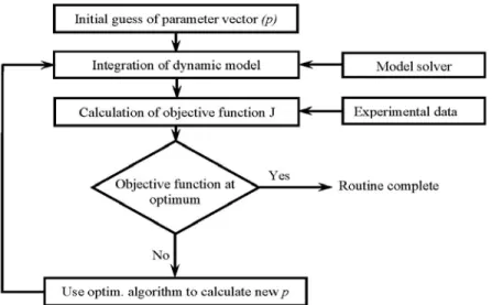
A control vector parameterization like approach for integration has been suggested such that the search space is discretized in time. By assuming a piecewise constant control, we have been able to integrate the model equations so that the objective function can be evaluated. Running a numerical constrained/unconstrained optimization technique on top of this space allowed us to obtain the values of decision variables, i.e. parameters in the kinetic models, after a reasonable set of iterations to satisfy a stopping criterion. Since no approximation polynomials or sensitivity functions were required, the calculations were substantially simplified.
Figure 1: Basic iteration routine for parameter estimation
The algorithm offers the possibility of employing different numerical optimization routines with ease to estimate the updated p in order to satisfy the particular needs of the model employed.
Model parameters were estimated by Quasi-Newton (QN), Nelder-Mead Simplex (NMS), Gauss-Newton (GN), Levenberg-Marquardt (LM), Sequential Quadratic Programming (SQP) algorithms by minimizing the objective function, which is the sum of squares of errors between the predicted and measured values for all of the state variables for a dynamic run as follows;
(
)
n m
2 ij o,ij i 1 j 1
J x x
= =
=
∑∑
− (5)where x: computed value, x0: observed value, n:
total number of state variables and m: total number
of observations. MATLAB 6.5 software package
and a 2.4 GHz Pentium 4 processor having 512 MB RAM were used for all computations.
PARES SOFTWARE
Software PARES (PARameter EStimation),
coded in MATLAB
TM
6.5 has been developed to implement the suggested parameter estimation technique. PARES is an interactive software system to identify parameters in differential algebraic equation system models. The program has ability to make parameter estimation with different optimization methods. For unconstraint optimization
problems, Gauss-Newton, Nelder-Mead Simplex, Levenberg-Marquardt or Quasi-Newton methods can be optionally used whereas sequential quadratic programming needs to be used for constraint optimization problems.
The program requires the input data in six main steps described as follows:
1. Model equations (user can enter any model, on the window provided as an M-file)
3. Initial, lower and upper bounds of the parameters
4. Starting, final and sampling times for experimental data
5. Number of state variables
6. Experimental measurements of state variables
The software, whose graphical user interface is shown in Figure 2, has also the ability to choose different objective functions (i.e. least square error, absolute error or standardized absolute error). It shows optimum model parameters, CPU time, objective function and the fit between experimental and predicted values of each state variable graphically. Contrary to the ERA software package, there is no limit on the number of parameters and state variables.
EXAMPLE PROBLEMS AND RESULTS
Although many linear and nonlinear models with varying degree of kinetic complexity have been tested, three examples are included here briefly to demonstrate the validity of the obtained results with literature for comparison reasons.
Example 1 represents a first-order reversible chain reaction in series, and was presented by Esposito and Floudas (2000). The reaction kinetic is expressed as,
3 1
2 4
k k
k k
A
⇔ ⇔
B C (6)All of the components are supposed to be measured, and therefore their concentrations are included in the model used. The dynamic model is written as
(
)
[
]
[
]
1
1 1 2 2
2
1 1 2 3 2 4 3
3
3 2 4 3 0 dx
p x p x ,
dt
dx
p x p p x p x
dt
dx
p x p x , x 1, 0, 0 t 0, 1
dt
= − +
= − + +
= − = ∈
(7)
where the state vector, x, is defined as [A, B, C], and parameter vector, p, is defined as [k1, k2, k3, k4].
Figure 3 depicted that the comparison of experimental and observed data using SQP for Example 1. The results were summarized in Table 1.
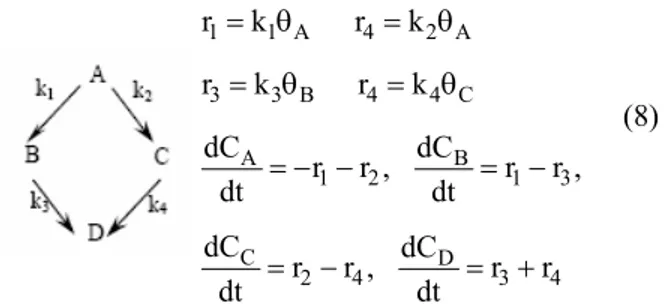
Example 2 tackles catalytic hydrogenation of cinnamaldehyde, which was previously investigated by Zamostny and Belohlav (1999). Reactions occurring in the system are indicated in the scheme as follows. The experiment was carried out in an isothermal, isobaric, stirred semi-batch reactor, the mass balance of which is given by the following equations.
1 1 A 4 2 A
3 3 B 4 4 C
A B
1 2 1 3
C D
2 4 3 4
r k r k
r k r k
dC dC
r r , r r ,
dt dt
dC dC
r r , r r
dt dt
= θ = θ
= θ = θ
= − − = −
= − = +
(8)
where r : reaction rate, k : rate constant, t : time, and
θi : catalyst surface coverage for i-th compound. The
parameter estimation problem was solved using different optimization routines.
Figure 4 shows that the predicted data fits, in a good agreement, with the experimental measurements. By increasing the complexity of the problem, SQP method becomes more effective than compared to those other methods. The results were summarized in Table 2.
0 0.1 0.2 0.3 0.4 0.5 0.6 0.7 0.8 0.9 1
0 0.1 0.2 0.3 0.4 0.5 0.6 0.7 0.8 0.9 1
Time min
S
tat
e v
a
ri
a
bl
es
, x
Exp.(x1) Pred.(x1) Exp.(x2) Pred.(x2)
Table 1: Optimization results for Example 1.
Parameters
Method Po Iter. Obj. Func. CPU(s)
P1 P2 P3 P4
P01 135 2.1125e-4 249.4 4.004 2.003 38.431 19.205
LM
P02 554 8.9698e-4 1321 4.003 1.997 38.571 19.331
P01 310 1.8897e-7 116.8 4.000 2.000 40.012 20.006
NM
P02 469 1.8897e-7 203.7 4.000 2.000 40.012 20.006
P01 13 1.9003e-7 22.2 4.000 2.000 40.000 20.000
QN
P02 27 0.0037 55.2 3.8947 1.877 194.521 100.18
P01 21 1.9012e-7 22.2 4.000 2.000 40.020 20.010
SQP
P02 71 1.8893e-7 97.9 4.000 2.000 40.007 20.003
EspositoandFloudas1a(2000) 338 3.367e-7 549.07 4.001 2.001 39.80 19.90
EspositoandFloudas1b(2000) 280 1.890e-7 1546.05 4.000 2.000 40.01 20.01
Optimum 4 2 40 20
Lower Bounds 0 0 10 10
Upper Bounds 10 10 50 50
1a
Collocation approximation
1b
Integration approximation Initial parameter set-1: P01
= 10 10 30 30 Initial parameter set-2: P02
= 50 50 150 150
Table 2: Optimization results for Example 2
Parameters Method P0 Iter. Obj. Func. Cpu (s)
P1 P2 P3 P4 P5 P6 P7
P01 12 0.3057672 17.9 0.078803 0.007757 0.015791 0.495315 1.287831 0.009937 0.001029
GN
P02 137 0.0187441 173.2 0.071800 0.006386 0.017744 3.970547 1.170721 3.968018 0.202995
P01 40 0.2520338 72.2 0.078583 0.006451 0.015966 0.500007 1.300065 0.010394 0.001072
LM
P02 57 0.0191650 57.1 0.079678 0.006379 0.017648 5.006390 1.475823 5.003202 0.255591
P01 802 0.0085128 211.2 0.073564 0.013398 0.013082 0.570624 1.525325 0.121945 0.032142
NMS
P02 1044 0.0145595 179 0.085655 0.005271 0.016290 11.72104 1.750016 0.000090 0.012230
P01 17 0.0069060 16.2 0.073912 0.009529 0.017131 0.453575 1.317102 0.075348 0.250904
QN
P02 - - - - -
P01 16 0.0069062 12.5 0.074040 0.009552 0.017094 0.472567 1.324329 0.072420 0.250316
SQP
P02 40 0.0069 27.5 0.073907 0.009568 0.017012 1.951910 1.325603 0.017675 0.249440
2a 0.0069454 - 0.074280 0.009840 0.017650 0.472100 1.305290 0.061976 0.271790
Optimum 0.073720 0.009190 0.017440 0.481300 1.294000 0.065660 0.260070
Lower Bounds 0.061708 0.006265 0.013372 0.178260 0.937730 0.000405 4.83e-17
Upper Bounds 0.090377 0.013552 0.022540 10.01100 2.014500 10.00600 0.511800
2a
Modified adaptive random search algorithm (Zamonstny and Belohlav (1999)) Initial parameter set-1: P01
= 0.08 0.009 0.018 0.5 1.3 0.01 0.001 Initial parameter set-2: P02
= 0.40 0.045 0.09 2.5 6.5 0.05 0.005
0 10 20 30 40 50 60 70 80 90
0 0.1 0.2 0.3 0.4 0.5 0.6 0.7 0.8 0.9 1
Time min
S
ta
te v
a
ri
ab
les
, x
Exp.(x1) Pred.(x1) Exp.(x2) Pred.(x2) Exp.(x3) Pred.(x3) Exp.(x4) Pred.(x4)
Example 3 The kinetic is a first-order irreversible chain reaction as presented by Esposito and Floudas (2000).
1 2
k k
A→ →B C
Only the concentrations of components A and B were measured; therefore, component C did not appear in the model used for estimation. The differential equation model takes the form
1 2
1 1 1 1 2 2
dx dx
p x , p x p x ,
dt = − dt = − (9)
[
]
[
]
0
x = 1, 0 t∈ 0, 1
where the state vector, x, is defined as [A, B], and parameter vector, p, is defined as [k1, k2]. The data
used in the study was generated with the p values of [5, 1].
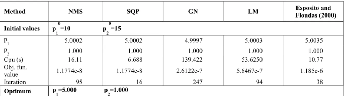
The parameter estimation problem was solved using different optimization methods. Figure 5 shows that the observed data fits the experimental measurements very well. The results were summarized in Table 3. According to these results, the number of iteration and CPU time of SQP method are much better than the other methods.
Table 3: Optimization results for Example 3
Method NMS SQP GN LM Esposito and
Floudas (2000)
Initial values p
1 0
=10 p
2 0
=15
p
1 5.0002 5.0002 4.9997 5.0003 5.0035
p
2 1.000 1.000 1.000 1.000 1.000
Cpu (s) 16.11 6.688 139.422 53.6250 10.77
Obj. fun.
value 1.1774e-8 1.1774e-8 2.6122e-7 5.6467e-7 1.185e-6
Iteration 95 16 247 94 38
Optimum p
1=5.000 p2=1.000
0 0.1 0.2 0.3 0.4 0.5 0.6 0.7 0.8 0.9 1
0 0.1 0.2 0.3 0.4 0.5 0.6 0.7 0.8 0.9 1
Time min
S
tat
e
v
a
ri
ab
le
s
,
x
Exp.(x1) Pred.(x1) Exp.(x2) Pred.(x2)
CONCLUSIONS
As reflected by the results, solution to such difficult dynamic optimization problems for parameter estimation seems to be effectively achieved by suggested approach. Particularly, Table 1 reveals that PARES software, which is capable of accomplishing the task with much less iterations and CPU time than previously published techniques, and furthermore the SQP method appears to be favourable to other numerical optimization routines.
REFERENCES
Agun, U., Optimization of feeding profile in baker’s yeast fermentation, M.S. Thesis, Ankara University, Ankara, Turkey (2002).
Albuquerque, J. S., and Biegler, L. T., Data reconciliation and gross error detection for dynamic system, AIChE Journal, 42 No.10, 2841 (1996).
Arora, N., and Biegler, L. T., Redescending estimators for data reconciliation and parameter estimation, Computers and Chemical Engineering, 25, 1585 (2001).
Bard, Y., Nonlinear Parameter Estimation, Academic Press, New York (1994).
Boggs, P. T. and Tolle, J. W., Sequential Quadratic Programming, Acta Numerica, Cambridge University Press, Cambridge, UK, pp. 1 (1995). Esposito, W. R. and Floudas, C. A., Global
Optimization for the Parameter Estimation of Differential Algebraic Systems, Ind. Eng. Chem. Res., 39, 1291 (2000).
Fletcher, R., Practical Methods of Optimization, Second Ed., Chichester: John Wiley and Sons, Inc. (1987).
Fukushima, M., A successive quadratic programming algorithm with global and superlinear
convergence properties, Math. Programming, 35, 253 (1986).
Hock, W. and Schittkowski, K., Test examples for nonlinear programming codes: No. 187, in Lecture Notes in Economics and Mathematical Systems, Heidelberg, Germany: Springer Verlag (1981).
Huybrechts, V. and Assche, G. V., OPTKIN- Mechanistic Modelling by Kinetic and Thermodynamic Parameter Optimization, Computers and Chemistry, 22, 413 (1998).
Neumann, G. A., Finkler, T. F., Cardozo, N. S. M. Secchi, A. R., Parameter estimation for LLDPE gas-phase reactor models, Braz. J. Chem. Eng., 24, No.2, 267 (2007).
Powell, M. J. D., A Fast Algorithm for Nonlinearly Constrained Optimization Calculations, Numerical Analysis, G. A.Watson ed., Lecture Notes in Mathematics, Springer Verlag, Vol. 630 (1978).
Stewart, W. E., Caracotsios, M. and Sorensen, J. P., Parameter Estimation From Multiresponse Data, AIChE J., 38, 641 (1992).
The Mathworks, Inc. (2003). www.mathworks.com. Tjoa, I-B. and Biegler, L. T., Simultaneous solution
and optimization strategies for parameter estimation of differential-algebraic equation schemes, Ind. Eng. Chem. Res., 30, 376 (1991). Vassiliadis, V. S., Sargent, R. W. H. and Pantelides,
C. C., Solution of a Class of Multistage Dynamic Optimization Problems. 1. Problems without Path Constraints, Ind. and Eng. Chem. Res., 33, 2111 (1994).
Yuceer, M, Karadurmus, E. and Berber, R., Simulation of river streams: Comparison of a new technique with QUAL2E, Mathematical and Computer Modelling, 46, No.1-2, 292 (2007). Zamostny, P. and Belohlav, Z., A Software for