Braz. J. Chem. Eng. vol.25 número4

ISSN 0104-6632 Printed in Brazil

www.abeq.org.br/bjche

Vol. 25, No. 04, pp. 777 - 788, October - December, 2008

Brazilian Journal

of Chemical

Engineering

DESIGN OF A MULTI-MODEL OBSERVER-BASED

ESTIMATOR FOR FAULT DETECTION AND

ISOLATION (FDI) STRATEGY: APPLICATION TO

A CHEMICAL REACTOR

Y. Chetouani

Université de Rouen, Phone: (0033)23528466, Fax: (0033)235147191, Rue Lavoisier 76821, Mont Saint Aignan Cedex, France.

E-mail: Yahya.Chetouani@univ-rouen.fr

(Received: February 1, 2007 ; Accepted : March 5, 2008)

Abstract - This study presents a FDI strategy for nonlinear dynamic systems. It shows a methodology of tackling the fault detection and isolation issue by combining a technique based on the residuals signal and a technique using the multiple Kalman filters. The usefulness of this combination is the on-line implementation of the set of models, which represents the normal mode and all dynamics of faults, if the statistical decision threshold on the residuals exceeds a fixed value. In other cases, one Extended Kalman Filter (EKF) is enough to estimate the process state. After describing the system architecture and the proposed FDI methodology, we present a realistic application in order to show the technique's potential. An algorithm is described and applied to a chemical process like a perfectly stirred chemical reactor functioning in a semi-batch mode. The chemical reaction used is an oxido reduction one, the oxidation of sodium thiosulfate by hydrogen peroxide.

Keywords:Safety; Reliability; Risk assessment; FDI method; Model-based approach; Extended Kalman Filter (EKF).

INTRODUCTION

A chemical process can only be implemented for industrial application if a complete study has been carried out to guarantee its safety and the quality of its products. Before this industrial stage, phenomena occurring during the chemical process are characterized to make sure that this process is the most adapted. However, plants in the chemical and biochemical industries are becoming larger and more complex. The growing safety and environmental demands are forcing industry to look for more powerful and new techniques for the detection of process faults. A fault is defined as an unexpected change of the system functionality which may be related to a failure in a physical component or in a system sensor or actuator. The early detection and

isolation of faults in engineering and industrial systems is a critical factor for avoiding product deterioration, major damage to machinery, loss of production, performance degradation, poor plant economy, environmental pollution and damage to human health or even loss of life.

Chetouani, 2006b). Model-based techniques all use mathematical models of the plant being monitored. A wide variety of these approaches have been proposed to tackle the isolation problem (Patton et al., 2000; Chen et al., 1999; Isermann et al., 1997). However, the conceptual realization of these models can vary according to the following approaches; the fault detection filter (Liberatore et al., 2006; Henry et al., 2005), the parity space (Isadi et al., 2005), parameter identification (Fantuzzi et al., 2002; Zogg et al., 2006), state estimation (Biagiola et al., 2006) and nonlinear techniques (Edelmayer et al., 2004; Korbicz et al., 2004). The model-based approach based on a Kalman filter has been used in different type of applications, like the on-line failure detection in nuclear power plants (Tylee, 1983); the on-line fault in a chemical reactor (Chetouani, 2004), in DC motors to predict failures by placing an exponential attenuator at the output end of the motor model to simulate aging failures, resulting in small prediction errors (Yang, 2002), or in the detection of faults in turnouts in the infrastructure elements of railway systems (García et al., 2003; Pedregal et al., 2004). Simani et al. (2006) used the EKF for the dynamic system identification and model-based fault diagnosis of an industrial gas turbine prototype. A model-based procedure exploiting analytical redundancy for the detection and isolation of faults in a gas turbine process was presented. The main point of their work consists of exploiting system identification schemes in connection with observer and filter design procedures for diagnostic purpose. Zhan et al. (2006) presented a model-based technique for the detection and diagnosis of gear faults under varying load conditions using the gear motion residual signal. A noise-adaptive Kalman filter-based Auto-Regressive (AR) model was fitted to the gear motion residual signals in the healthy state of the gear of interest. It consists of fitting an AR model to gear motion residual signals and takes advantage of the NAKF to decorrelate the signal to produce a white Gaussian sequence. Pedregal et al. (2006) developed a complex prediction model based on the algorithm Kalman filter for vibration data within the state space class applied to real data in the petrochemical industry. The core of the system is a model to forecast the state of the machine using data provided by the condition monitoring system at each moment in time. Feil et al. (2006) presented a monitoring system based on Kalman filtering for process transitions. They used a model-based state-estimation algorithm to detect the changes in the correlation among the state-variables. Brännbacka et al. (2004) developed an advanced model to track iron and slag levels in the blast furnace hearth. The liquid level estimation problem is tackled

In this paper, the basic idea of the adopted approach is to reconstruct the outputs of the system from the measurement using observers and using the residuals for fault detection (Mehra et al., 1971; Franck, 1990; Chetouani, 2004). This study also shows a methodology for tackling the isolation issue of fault causes by combining the last technique and the technique using the multiple Kalman filters for a nonlinear dynamic system. The usefulness of this combination is the on-line implementation of all the models of fault dynamics if the statistical decision threshold on the standardized innovation exceeds a fixed value. In other cases, one extended Kalman filter is enough to estimate the process state in order to avoid the high numerical integration of all models. After describing the system architecture and the proposed methodology of the FDI, we present a realistic application in order to show the technique's potential. The purpose is to develop and test the FDI method on real incident data, to detect the occurrence of change, to pinpoint the moment it occurred and to locate the fault cause. The experimental results demonstrate the robustness of the FDI method.

The structure of the paper is as follows. First, the description of the FI strategy by using the multiple Kalman filters is presented. Then the FD strategy by using the standardized innovations is presented followed by the description of the proposed FDI method. Then a comprehensive experimental validation of the proposed method is presented. Finally, conclusions are drawn in the last section.

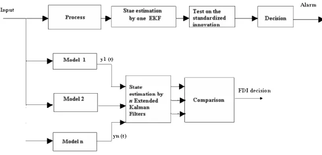
FAULT ISOLATION STRATEGY BY USING THE MULTIPLE KALMAN FILTERS

A FDI system should perform two tasks, namely fault detection and fault isolation. The purpose of the fault detection module is to determine that a fault has occurred in the system. The second task is devoted to locate the fault cause. To achieve this aim, all the available information from the process should be collected and processed to detect any change from nominal behavior of the process. Model-based fault isolation relies on mathematical models of the plant to identify a discrepancy between the nominal plant and the plant when a fault occurs (Isermann, 2005). The detection of faults is usually accomplished by evaluating the residuals that are sensitive to the fault’s occurrence in the process dynamics. In the case of a normal behavior, the residuals have properties that are known a priori. Hence, any sudden or abrupt change in the value of any control parameter of the process implies some deviation of those properties from the normal mode profile. Fig. 1 shows the fault isolation method based on the analysis of the residuals’ evolution between the real output and the output estimated by the extended Kalman filter. This filter is an effective tool for stochastic estimation of the state from noisy measurements. Because of its relative simplicity and robust nature, the Kalman filter has been widely used to obtain estimates of the state variables in practice. The filter’s number is defined from the exhaustive list of all the models of faults and the model of the normal behavior of the process.

The multiple filters method allows establishing a link between the detected anomalies during the process and a given situation of the process. It consists of having the observations processed by a set of EK filters (King et al., 1990). Each EKF corresponds to an assumption of a particular fault. {y1(t)…yn(t)} represent the models of faults. During normal functioning, the EK filters generate innovations which must be low. They depend only on the intrinsic errors and the random variations of the measurement equipment. In other cases where the process dynamics are not respected, these same signals evolve differently according to the magnitude of the effect of the fault on the general state of the plant. Consequently, the aim of this method consists of determining the nearest filter which generates the lowest innovation.

By supposing that the behavior of a nonlinear process is described by a finished set of models indexed i 1,...., N= ; and by the input u(k) and the output z(k) for k=1, 2,..., the dynamics of a nonlinear process can be expressed by the following:

i i i i i

x (t) =f (x (t), u (t), t)+w (t) (1)

i i i k i

z (k)=h (x (t ))+v (k) k=1, 2, ...

where x∈ℜn is the state vector, with an initial value of x , z is the measurement vector, w(t) is the ₀ system noise representing modeling error and unknown disturbances, and v(k) is the measurement noise. Both system and measurement noises are assumed to be independent random white noises with zero mean and covariance matrices, respectively Q and R. The functions f and h denote, respectively, a nonlinear function of the state and the output. The extended Kalman filter is essentially a set of mathematical equations that aims at minimizing the estimated error covariance in the state estimator (Hovland et al., 2005). This estimation by EKF is given by the following equations:

The Kalman gain is:

T T 1

k k k ˆk k ˆk k k ˆk

K =P H− (x )(H (x )P H− − − (x )− +R)− (2)

ƒ The a posteriori state estimate is:

k k k k k k

ˆ ˆ ˆ

x+=x−+K (y −h (x ))− (3)

where γ =_k (y_k−h (x ))_k ˆ_k− is the innovation between the measured output and the estimated one.

ƒ The a posteriori state covariance is:

k k k ˆk k

P+ = −(I K H (x ))P− − (4)

where H(x(t), t) is the Jacobian matrix of the ˆ partial derivative of h according to the state vector:

i ij

j _{x(t) x(t)ˆ}

h (x(t), t) ˆ

H (x(t), t)

x (t) =

∂ =

∂ (5)

Under normal operating conditions, the innovation γ =_k (y_k−h (x ))_k ˆ_k− is a white noise sequence with a zero mean and a variance:

T

k (H (x )P Hk ˆk− k− k (x )ˆk− R)

η = + (6)

By noting that the model i is the model which represents the dynamics of the real system, its probability can be defined on-line according to a hypothesis test. Unlike the standard Kalman filter, this method has for input the set

(

)

i i i i i

I (k)= u (0),..., u (k 1),− z (1),..., z (k) and for output the probability of each model. By applying Bayes’ law, the probability of each model is:

(

)

(

)

i i i i i

i _N

j j j j j

j 1

p z (k 1/ H ), I (k), u (k) p (k) p (k 1)

p z (k 1/ H ), I (k), u (k) p (k) =

+ + =

+

∑

where the density of the conditional probability

i i i i

p(z (k 1/ H ), I (k), u (k))+ is calculated according to the nature of the noise. Its distribution follows a normal law:

(

)

(

)

i

i i i i

T 1

i i

1/ 2 m / 2

i

p z (k 1/ H ), I (k), u (k)

1

exp (k 1) (k 1) (k 1) 2

(2 ) det( (k 1) −

+ =

_{− γ + η + γ +} 

 

 

π η +

(8)

FAULT DETECTION STRATEGY BY USING THE STANDARDIZED INNOVATIONS

Analysis of the generated innovation is required for fault detection. In the absence of faults, the innovation value is near zero. A fault causes the process to behave differently from normal model prediction, and the filter, which compares the model and the process, generates large innovation. Faults are detected by deviation of the innovation from this normal value. In practice statistical analysis of innovation such as mean moving average mean, whiteness ratio can also be used as the fault detection signal. But in the case study (Chetouani, 2004), it was observed that the innovations are themselves a good indication of the process state (normal or faulty). In this case, the statistical threshold based on innovations allows delimiting two distinct regions; the first region is called the safe region where the innovation variation is considered to be acceptable. The second region is not acceptable (fault region) and is where the innovation variation exceeds the statistical threshold. Considering a fault region π in the sample space ℜn, an acceptable region C_π is defined as the complement of π in ℜn. Let M be a point of size n

representing the sample. The sampling corresponds to a real representation of the process. Notice that it is convenient to use the standardized innovation sequence for the standardized hypothesis of statistical tests (Chetouani, 2006a). This sequence is expressed as follows:

T 1/ 2

k k k k k k

1/ 2

k k k k k

ˆ ˆ

s (H (x )P H (x ) R)

ˆ

(y h (x )) ( )

− − − −

− −

η = +

− = η γ (9)

with

T

j k jk

E( sη ηs )= δI (10)

δ and I represent, respectively, the Kronecker symbol and the identity matrix. ηs_k has a zero mean and an unit variance. Any deviation from the normal behavior causes a substantial change of these statistical properties. A test on the mean of the normal law N(0, I) is carried out to verify whether the standardized innovation sequence (Chetouani, 2006a) has a zero mean. The latter is estimated by:

N j j 1

1

ˆ s s

N ₌

η =

∑

where N is the sample size, which depends on the system dynamics. The size of the representative observation sample depends on the system response;

if the latter is slow, the size will be large. Otherwise, when the dynamics evolves rapidly, samples will be taken quickly in order to enable the decision to be made as early as possible. sη refers to the true mean of the

sample. Under the hypothesis (H ), ˆ s_o η has a gaussian distribution with a zero mean and a covariance

T

ˆ ˆ

E( s s )η η =I / N. However, beyond a given level of acceptance, such as above α (‘non-normal’ hypothesis

1

H ), the ‘normal’ hypothesis (H ) is rejected: _o

ˆ s

η > α (12)

The threshold α depends on the probability of false alarms. Threshold limits can be defined for innovations for a normal behavior. Threshold limit selection, in most cases, is dependent on the process at hand (Himmelblau, 1978). The threshold hypothesis accounts for innovation changes due to noise and some process-model mismatch. In other words, threshold limits can be defined and based on minimum process deviations that are not acceptable.

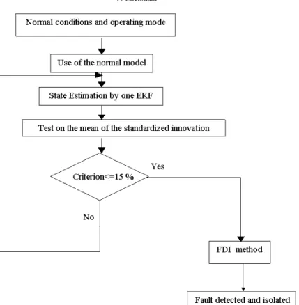
THE PROPOSED FDI APPROACH

Figure 2: The proposed FDI approach

APPLICATION OF THE PROPOSED FDI APPROACH

Experimental Device: Chemical Reactor

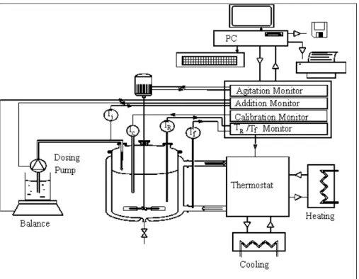
The chemical reactor represented in Fig. 3 works under atmospheric pressure. It is a glass-jacketed reactor with a tangential input for heat transfer fluid. The capacity of the reactor is two liters. It is equipped with an electrical calibration heating, a stirring system (anchor) and an input system (two dosing pumps and two scales, with temperature measurement at input). It is also equipped with Pt100 temperature probes. Five probes are inserted through the chemical reactor in the reaction mass, in the cooling, in the condenser and in the flow rate introduction. The heating-cooling system, which uses a single heat transfer fluid, works within a temperature range from -15 to +200 °C. Supervision software allows the fitting of the parameters and their instruction value. The parameters introduced in the supervision system are the control modes of the reaction mass temperature (isothermal or slope of the temperature) and of the jacket fluid (constant or slope of the temperature). The distillation mode (the difference between the reaction mass temperature and the fluid jacket temperature is maintained

constant) can also be introduced. Supervision software also allows the regulation of the flow rate introduction and the stirring rate of the reactor. It displays and stores data during the experiment for further exploitation.

Chemical Reaction Choice

In order to illustrate the proposed FDI approach, a chemical synthesis in a laboratory-size reactor was carried-out. The reaction chosen is a very exothermic oxido-reduction one (Aime, 1991), the oxidation of sodium thiosulfate by hydrogen peroxide. This reaction can be expressed by the following equation:

2 2 3 2 2 2 3 6

2 4 2

N a S O 2 H O 0 .5 N a S O

0 .5 N a S O 2 H O

+ → +

+ (13)

This equation is written as: 2A+ →B 0.5C+0.5D+2E, where the following notations are adapted: A : hydrogen peroxide

2 2

H O ; B: sodium thiosulfate Na S O ; C : _{2 2 3} sodium persulfate Na S O ; D : sodium sulfate _{2 3 6}

2 4

Figure 3: Diagram of the chemical reactor

Chemical Reactor Modeling

In order to guarantee that faults can be detected and isolated, mathematical models of the process under investigation are required, either in state space or input-output form. State space descriptions generally provide mathematically rigorous tools for system modelling and residual generation that may be used in fault detection of industrial systems, both for noise-free measurements and noisy data environment. The dynamic behavior of the chemical reactor is modeled by a system of differential equations translating molar and heat balances in the reactor. The model used is based on the following hypotheses (Chetouani, 2004):

ƒ The reactor is perfectly stirred: reaction mass temperature and concentrations are homogeneous through the mass volume;

ƒ No phase change in the reaction mass;

ƒ The density, the specific heat of the cooling and the reaction mass heat are independent of the temperature.

ƒ By taking into account the thermal inertia of the wall, three energy balances (14, 15 and 16) were established, respectively, in the reaction mass, in the jacket fluid and in the reactor wall.

(

)

)

(

(

)

(

)

1

F j

R

R

R R R R R w r R

E RT

0 o o

T

j j a R

T

dT (t)

m Cp h A T (t) T (r , t) d t

k e n (M ) / V n (Z ) V H

F Cp dT Kc T T (t)

=

−

β α

= − − −

−χ −χ ∆

+

∫

(14)

(

)

(

)

f

f f f f fe f

f f w r R e f

d T (t)

m Cp m Cp T (t) T (t) d t

h A T T (t)

•

= +

= − +

−

(15)

2

w w

2

2

w w

2

w

T (r, t) 1 T (r, t)

r r

r

T (r, t) 1 T (r, t)

a t

z

∂ ₊ ∂ ₊

∂ ∂

∂ ₌ ∂

∂ ∂

(16)

With boundary conditions in ℜ(O, r, z=0):

1 1

w R r R e

where

(

)

1 1

T (r, t) T (r, t)

R e ln R = − = + µ =  +      (18)

(

)

1 1

T (r,t) ln(R e) T (r,t) ln(R )

R e ln R = + − = + τ =  +      (19)

t>0

(

)

1 w

R R R w r R w R

r R T (r,t)

h A T (t) T (r,t) A

t =

= ∂

− = −λ

∂ (20)

(

)

1 w f f w r R e f w f

r R e T (r,t)

h A T (r,t) T (t) A

t = +

= + ∂

− =−λ

∂ (21)

Using the normalized reaction extent (Villermaux, 1993), the mass balance in the reaction mass can be written according to an Arrhenius law:

)

(

(

)

k exp( E / RT ) M Z dt V

β α

χ = − − χ − χ (22)

Resolution of the Chemical System

The constituent order values for the reactants are

σ = 1.5 and β = 0.6 when the concentration ratio between hydrogen peroxide and sodium thiosulfate is maintained greater than 1.96 during the reaction (Cohen et al., 1962). Under the same operating conditions as those of Cohen et al. (Cohen et al., 1962) and by assuming that the rate coefficient is governed by the Arrhenius law, Aime (Aime, 1991) has estimated the kinetic parameters (frequency coefficient k = (7.25_{o ±}0.5) × 1011 L/mol.s and activation energy E = 79002±1254 J/mol), as well as the thermodynamic reaction enthalpy (∆H = -563±10 kJ/mol). The wall equation (16-21) is used in order to improve the model. In practice, the model of a system provides only an approximation of the real behavior. Because the observer is built from this model, the provided state and the output are sensitive to the errors coming from the difference between the system and its model. This point is particularly

significant if one is interested in fault detection and isolation. Indeed, the tests are established by analyzing the reconstruction error, which is sensitive to the detected faults and also to the modeling errors.

Before solving equations (14, 15 and 22) by the Runge-Kutta-Fehlberg method (Forsythe et al., 1977), the equation system for the heat balance in the reactor wall (16, 20 and 21) is transformed into an algebraic equation system. By employing the finite difference method under its explicit formulation, equations (16, 20 and 21) become, according to the numerical scheme in Fig. 4:

ƒ Temperature of the reaction mass for an interior nodal point (R₁< <r R₁+e):

n 1 w n

i w 2 i

n n

w

w ₂ i 1 w ₂ i 1

a t t

T 1 2a T

r r r

a t

t t

a T a T

r r r r + + −  ∆ ∆  = −_ − _∆ _ + ∆    ∆ ₊ ∆  ₊ ∆       _{∆ ∆}   _∆      (23)

ƒ where the subscript refers to the interior nodal point and the exponent refers to the time step. The boundary temperature of the reactor wall at r =R₁ is given as follows:

n 1 n n n

i R R i 1 R i

1

T 2Fo Bi T T Bi 1 T

2Fo + −     = _ + +_ − − _{ }  

  (24)

ƒ The boundary temperature of the reactor wall at

1

r = +R e is given as follows:

n 1 n n n

i f f i 1 f i

1

T 2Fo Bi T T Bi 1 T

2Fo + −     = _ + +_ − − _{ }  

  (25)

R1+e

R1

Reaction mass Wall Cooling

r = 0 r = R1 r = R1+e

Middle 1 Middle 2 Middle 3

Figure 4: Scheme of the numerical resolution

FDI Results

In order to illustrate the pertinence of the proposed FDI approach, it is applied to detect and locate a fault due to a sudden change, which occurs at 500 s, of the flow cooling during the phase of preheating of a reaction mass. The normal conditions are chosen corresponding to the flow Qv_n= 0.40.10-3 m3.s-1 and as non-normal conditions those which correspond to the flow Qv_fault= 1.10.10-3 m3.s-1. Theoretically, this last flow, which provides the measurement dynamics y , is unknown by the _s operator. The aim of the FDI method is to identify it by comparing its dynamics with those given in real-time by the mathematical library of different models. For this purpose, different dynamics corresponding to different flows of the cooling are built. This flow change does not modify the structure of the model equations, only the partial transfer coefficient h is _f modified. The selected flows of the cooling are as follows (Table 1).

The results of different simulations are given as follows (Fig. 5).

The evolution of the probability is conditioned by

the evolution of the innovation (Fig. 6). The latter is processed by the EKF to detect an actual fault condition, rejecting any false alarms caused by noise or spurious signals. The convergence of the innovation depends on the R / Q ratio. In fact, the knowledge of these two variances constitutes a means to adjust the EKF. It represents an indication of the filter’s degree of dependence on the measurements; if R is small and Q is large, then information coming from the measurements is preponderant in the estimation, and if R is large and

Q small, the filter gives preference to the model rather than to measurements (Chetouani, 2006a).

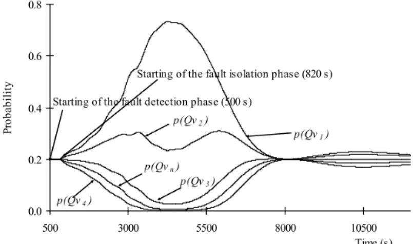
By analyzing the probability results (Fig. 7), it is observed that the fault isolation phase starts at 820 s, i.e., 320 s after the start of the fault detection phase, in order to avoid numerical calculations and false alarms. In addition, it is noted that the fault dynamics

s fault

y =f (Qv ) is close to that corresponding to the flow y_s =f (Qv )₁ because of the probability p(Qv ) , ₁ which is most important. The probability of the other models decreases considerably according to their respective variation compared to the output

s fault

y =f (Qv ), as shown in Fig. 7.

290 300 310 320 330 340

0 2000 4000 6000 8000 10000 12000 14000

Time (s)

T

e

m

p

e

ra

tu

re

(

K

)

Qv1

Qv2

Qv3

Qvn

Qv4

ys

Table 1: Selected flows of the cooling

Volumic flow ( m3.s-1 ) 1.33.10-3 0.80.10-3 0.60.10-3 0.20.10-3

Dynamics Qv 1 Qv 2 Qv 3 Qv 4

-0.50 -0.40 -0.30 -0.20 -0.10 0.00 0.10 0.20

500 3000 5500 8000 10500

Time (s)

In

nova

ti

o

ns

Qv1

Qv2

Qv3

Qvn

Qv4

Starting of the fault isolation phase (820 s) Starting of the fault detection phase (500 s)

Figure 6: Evolution of the generated innovations by the EK Filter

0.0 0.2 0.4 0.6 0.8

500 3000 5500 8000 10500

Time (s)

P

roba

bi

li

ty

p(Qv1)

p(Qv2)

p(Qv3)

p(Qvn)

p(Qv4)

Starting of the fault isolation phase (820 s) Starting of the fault detection phase (500 s)

Figure 7: Evolution of the different probabilities

CONCLUSION

In this paper, a model-based fault detection and isolation method for nonlinear systems has been considered, based on the idea of generating residuals. The proposed method requires physical knowledge of the process under observation. First an accurate model of the process dynamics has been constructed according to all the available information for the studied system. An extended Kalman filter is used for state estimation and residual generation. Faults are detected by a statistical threshold and isolated by using a combination of two decision methods. This evaluation is accomplished by means of a bank of

model-based approach. However, in practical applications, especially when considering large plants and complex systems, the straightforward application of such FDI techniques may be difficult. Thus, these models are often very nonlinear and very complex, and they can exploit hybrid structures to describe accurately the behavior of the real-target system. A viable and easy procedure for practical application of this technique is really necessary in complex applications.

ACKNOWLEDGEMENT

I acknowledge the critical comments of the anonymous reviewers for their very good comments, which greatly improved the manuscript. I would like to thank the edition staff for helping with the English of this manuscript.

NOMENCLATURE

A Exchange area m2 ko frequency coefficient m3.mol-1.s-1 E Energy activation J.mol-1 Cp Specific heat J.kg-1.K-1

e Wall thickness m

F Flow feeding mol.s-1 H Heat transfer coefficient W.m-2.K-1 Kc Conductance W.K-1

N Mole number mol

M Molar mass kg.kmol-1

m Mass kg

m• Flow rate kg.s-1 R Ideal gas constant J.mol-1.K-1

R1 Reactor radius m

R Reaction rate mol.m-3.s-1

T Temperature K

T Time s

V Volume m3

Subscript

f Fluid jacket R Reactor

W Wall A ambient Fe fluid inlet

Greek Letters

ρ Density kg.m-3

χ Normalized reaction extent (-)

H

∆ Reaction enthalpy kJ.mol-1

∆

REFERENCES

Aime, N., Aide à la conduite sûre des réacteurs chimiques discontinus en marche normale ou incidentelle vis-à-vis du danger d’emballement thermique, Ph.D. Thesis, Université de Technologie de Compiègne (1991).

Alessandri, A., Fault diagnosis for nonlinear systems using a bank of neural estimators, Computers in Industry, 52, 271-289 (2003).

Bhagwat, A., Srinivasan, R., Krishnaswamy, P. R. Multi-linear model-based fault detection during process transitions, Chemical Engineering Science, 58, 1649-1670 (2003).

Biagiola, S., Solsona, J., State estimation in batch processes using a nonlinear observer, Mathematical and Computer Modelling, 44, 1009-1024 (2006).

Brännbacka, J., Saxén, H., Novel model for estimation of liquid levels in the blast furnace hearth, Chemical Engineering Science, 59, 3423-3432 (2004).

Chen, J., Patton, R.J., Robust model-based fault diagnosis for dynamic systems, Kluwer Academic Publishers (1999).

Chetouani, Y., Fault detection in a chemical reactor by using the standardized innovation, Process Safety and Environmental Protection, 84, 27-32 (2006a).

Chetouani, Y., Application of the generalized likelihood ratio test for detecting changes in a chemical reactor, Process Safety and Environmental Protection, 84, 371-377 (2006b). Chetouani, Y., Fault detection by using the

innovation signal: application to an exothermic reaction, Chemical Engineering and Processing, 43, 1579-1585 (2004).

Cohen, W. C., Spencer, R., Determination of chemical kinetics by calorimetry, Chem. Eng. Prog., 58, 40-44 (1962).

Edelmayer, A., Bokor, J., Szabo, Z., Szigeti, F., Input reconstruction by means of system inversion: a geometric approach to fault detection and isolation in nonlinear systems, Int J Appl Math Comput Sci, 14, 189–199 (2004).

Feil, B., Abonyi, J., Nemeth, S., Arva, P., Monitoring process transitions by Kalman filtering and time-series segmentation, Computers & Chemical Engineering, 29, 1423-1431 (2005). Forsythe, G. E., Malcolm, M., Moler, C., Computer

Methods for Mathematical Computations, Prentice-Hall, New Jersey (1977).

Frank, P. M., Fault diagnosis in dynamic systems using analytical and knowledge-based redundancy. A survey and some new results, Automatica, 3, 459-474 (1990).

García, F. P., Schmid, F., Conde, J., A reliability centered approach to remote condition monitoring. A railway points case study, Reliability Engineering & System Safety, 80, 33– 40 (2003).

Henry, D., Zolghadri, A., Design of fault diagnosis filters: A multi-objective approach, Journal of the Franklin Institute, 342, 421-446 (2005).

Himmelblau, D. M., Fault detection and diagnosis in chemical and petrochemical processes, Elsevier, New York (1978).

Hovland, G. E., Von Hoff, T. P., Gallestey, E. A., Antoine, M., Farruggio, D., Paice, A. D. B., Nonlinear estimation methods for parameter tracking in power plants, Control Engineering Practice, 13, 1341-1355 (2005).

Isermann, R., Model-based fault-detection and diagnosis – status and applications, Annual Reviews in control, 29, 71–85 (2005).

Isermann, R., Ballé, P., Trends in the application of model-based fault detection and diagnosis of technical processes, Control Eng Pract, 5, 709– 719 (1997).

Izadi, I., Zhao, Q., Chen, T., An optimal scheme for fast rate fault detection based on multirate sampled data, Journal of Process Control, 15, 307-319 (2005).

Jang, D-S., Choi, H-L., Active models for tracking moving objects, Pattern Recognition, 33, 1135-1146 (2000).

King, R., Gilles, R., Multiple filter methods for detection of hazardous states in an industrial plant, AIChE, 11, 1697-1706 (1990).

Korbicz, J., Koscielny, J. M., Kowalczuk, Z., Cholewa, W., Fault diagnosis: models, artificial intelligence, applications (1st ed.), Springer-Verlag (2004).

Li, J., Xu, N. S., Su, W. W., Online estimation of stirred-tank microalgal photobioreactor cultures based on dissolved oxygen measurement,

Biochemical Engineering Journal, 14, 51-65 (2003). Liberatore, S., Speyer, J. L., Hsu, A. C., Application

of a fault detection filter to structural health monitoring, Automatica, 42, 1199-1209 (2006).. Mehra, R. K., Peschon, J., An introduction approach

to fault detection and diagnosis in dynamic systems, Automatica, 5, 637-640 (1971).

Nyberg, M., Stutte, T., Model based diagnosis of the air path of an automotive diesel engine, Control Engineering Practice, 12, 513-525 (2004).

Patton, R. J., Frank, P. M., Clark, R. N., Issues of fault diagnosis for dynamic systems, Springer-Verlag, London (2000).

Pedregal, D. J., Carnero, M. C., State space models for condition monitoring: a case study, Reliability Engineering & System Safety, 91, 171-180 (2006).

Pedregal, D. J., García, F. P., Schmid, F., RCM2 predictive maintenance of railway systems based on unobserved components models, Reliability Engineering & System Safety, 83, 103-110 (2004). Shi, P., Liu, H., Stochastic finite element framework

for simultaneous estimation of cardiac kinematic functions and material parameters, Medical Image Analysis, 7, 445-464 (2003).

Simani, S. Fantuzzi, C., Dynamic system identification and model-based fault diagnosis of an industrial gas turbine prototype, Mechatronics, 16, 341-363 (2006).

Tylee, J. L., On-line failure detection in nuclear power plant instrumentation, IEEE Trans Automatic Control, 3, 406-415 (1983).

Villermaux, J., Génie de la réaction chimique- conception et fonctionnement des réacteurs, Lavoisier, Paris (1993).

Yang, S. K., An experiment of state estimation for predictive maintenance using Kalman filter on a DC motor, Reliability Engineering & System Safety, 75, 103-111 (2002).

Yang, S. K., Liu, T. S., State estimation for predictive maintenance using Kalman filter, Reliability Engineering & System Safety, 66, 29-39 (1999).

Zhan, Y. Makis, V., A robust diagnostic model for gearboxes subject to vibration monitoring, Journal of Sound and Vibration, 290, 928-955 (2006).