Data Stream Based Algorithms For Wireless Sensor Network Applications

(1)

Data Stream Based Algorithms For Wireless Sensor

Network Applications

Andr L.L. de Aquino

1

, Carlos M.S. Figueiredo

1,2

, Eduardo F. Nakamura

1,2

Luciana S. Buriol

3

, Antonio A.F. Loureiro

1

, Antnio Otvio Fernandes

1

, Claudionor J.N. Coelho Jr.

1

_{Department of Computer Science}

Federal University of Minas Gerais

Belo Horizonte, MG, Brazil

Email:

{alla,mauricio,nakamura,loureiro,otavio,coelho}@dcc.ufmg.br

2

_{FUCAPI – Research and Technological Innovation Center}

Manaus, AM, Brazil

3

_{Institute of Informatics}

Federal University of Rio Grande do Sul

Porto Alegre, RS, Brazil

Email:

buriol@inf.ufrgs.br

Abstract— A wireless sensor network (WSN) is energy con-strained, and the extension of its lifetime is one of the most important issues in its design. Usually, a WSN collects a large amount of data from the environment. In contrast to the conventional remote sensing – based on satellites that collect large images, sound files, or specific scientific data – sensor networks tend to generate a large amount of sequential small and tuple-oriented data from several nodes, which constitutes data streams. In this work, we propose and evaluate two algorithms based on data stream, which use sampling and sketch techniques, to reduce data traffic in a WSN and, consequently, decrease the delay and energy consumption. Specifically, the sampling solution, provides a sample of only logn items to represent the original data ofn elements. Despite of the reduction, the sampling solution keeps a good data quality.

Simulation results reveal the efficiency of the proposed meth-ods by extending the network lifetime and reducing the delay without loosing data representativeness. Such a technique can be very useful to design energy-efficient and time-constrained sensor networks if the application is not so dependent on the data precision or the network operates in an exception situation (e.g., there are few resources remaining or there is an urgent situation).

I. INTRODUCTION

A wireless sensor network (WSNs) [1], [2], [3] usually generates data that arrives at a sink node (gateway) in an online fashion, it is unlimited and there is no control in the arrival order of the messages to be processed. Data with this characteristic is called data stream. However, there is a difference between sensor stream and traditional stream. The sensor streams are only samples of the entire population, usually imprecise and noisy, and typically of moderate size. On the other hand, in traditional stream the entire population is usually available, the data is exact, error-free and huge [4].

Recent research in traditional data stream algorithms try to establish their lower bounds. The main metrics analyzed are time and communication complexities [5], [6], [7]. There are proposals that present specific data stream applications, which are modeled using data stream algorithms. For example, finding the rarity and similarity in a data stream or counting the triangulation in a Web graph [8], [9], [10], [11]. Indyk [12] proposes a data stream algorithm (implemented by Zhao [13]) that uses a family of hash functions called min-wise [14] to compute properties in data streams. This algorithm uses O(logn)bits to represent a hash index. The Indyk’s algorithm computes aδ−errorand anǫ−approximationfor the index found.

There are many techniques, in traditional streaming, which reduce the volume of data that can be applied or adapted to a sensor stream. Examples of some techniques are: sampling, histograms, sliding windows, sketches, and wavelets. Applica-tions of each one of these techniques generates data similar to the real ones. The similarity of the generated data and the real data depends on how the technique adopted is conduced and the application requires to be computed.

There are two main types of applications for WSNs: mon-itoring and actuating applications. In monmon-itoring applications, the sensor nodes only process the sensing data. In actuating applications, nodes can interfere in the monitored environ-ment [15], [16]. In both scenarios, we can apply data stream techniques to process the sensor stream, in the monitoring case, or to compose stream queries, in the actuating case.

The most common sensor stream solutions consider the network as a distributed database. In this case, the network abstraction is based on a Data Stream Management System (DSMS). These applications are concerned with how queries

(2)

can be answered [17], [18], [19], [20]. Some proposals use the amount of resources available at a DSMS and apply it to extract management information from the WSN, such as energy and node location [21], [22]. However, current DSMS’s are not suitable for WSNs, since sensor nodes have too few resources.

If a node sends all its measurements, it will spend much energy, and part of the data will probably be delayed or lost. To avoid this situation, part of the data is just not processed. A data stream algorithm based on sampling processes only part of the data, producing data similar to the original one. A data stream algorithm that sketches data, reduce it through a data sketch such as calculating the minimum, maximum and average of a data [18] or counting the data frequency. Histogram is another technique used to capture the distribution or the data behavior, i.e., data is analyzed and accumulated according to its category in such a way that only one data in this distribution is stored [23].

In the literature, we can find some proposals for WSNs that are based on data stream techniques. In some cases the application performs an adaptive sampling of the data sensing [24], [25], [26], [27]. In other cases, the solutions are based on data reduction or aggregation, often based on correlated information about the data sensing [28], [29], [30]. In this work, we follow that strategy to reduce the network traffic but keeping the data quality and its representativeness. We propose two algorithms based on data stream for WSNs that use sampling and sketch of data. Using our solutions it is possible to reduce data traffic and, consequently, the delay and energy consumption in a WSN. This work presents a way to deal with energy and time constraints at the application level, as a complementary view of solutions that treat this problem in the lower network levels. In special, the sampling algorithm aims to choose the ideal sample size for processing data streams.

This work is organized as follows. In Section II, we intro-duce the data stream problem. Next, in Section III, we present the algorithms based on data stream for sensor network data. Experimental results are given in Section IV, and Section V concludes this study and presents the future work.

II. PROBLEMDEFINITION

The problem addressed in this work can be stated as follows: Problem Statement: Given a sensor stream, we want to meet WSN requirements by reducing data traffic (using techniques based on data stream) and assuring a minimum data quality that allows to decrease energy consumption and delay.

This problem can be further assessed by answering the following questions:

• Data quality: How can we evaluate the quality of the

processed data? In some applications, the main goal of a WSN is to deliver sensed data to an observer. Due to the network limitations and the data characteristics only samples or sketches of the data stream are sent. Thus, we must evaluate if the transmitted data is representative. To perform this evaluation we can use statistics tests to know

whether the original sensor stream and the sampled one are equivalent, and also compare the distance between the average of their data values.

• Data reduction: How much data can be reduced without

compromising the application objectives? In the sampling case, we need to identify the minimum data sample that can be used in specific application. In this sense, we use a sample oflognelements to represent a population ofn elements while maintaining the data quality. Other sample sizes can be used according to the application requirements. When we use the sketch, it represents all data, using the fixed size. In this case we loose the data sequence.

• Losses vs. benefits: What is the relationship among the

data-quality loss and the benefits for attending network requirements? By reducing the stream size using a sam-pling technique there is an impact on the data quality, which is an important aspect for the application. However, the higher the data is reduced the more benefits are achieved for the network requirements such as delay and energy. The decision about which aspect is more important depends on the application requirements, and so the evaluation of this relationship is important. In the sketch case we loose the sequence of data, however we have a good approximation of the original sensor stream where the data can be regenerated artificially in the sink. All these questions must be answered to conceive a proper solution to sensor stream. To address these answers, the scope of this work considers the following assumptions:

• Sensor network topology: We consider a flat network

composed of homogeneous sensor nodes with a single sink node (gateway) to receive and process data from source nodes. We use a common tree-based routing solu-tion to evaluate the network behavior. The data evaluasolu-tion is computed when data arrives in the sink.

• Data stream processing: The streams are processed only

by the source nodes, i.e., each source processes its own data stream and sends the results towards the sink node.

• Data stream generation: The streams are generated

continuously at regular intervals (periods) of time and follow a normal distribution to represent their values.

III. SENSORSTREAMSOLUTIONS

To address the problem stated above, we need to design algorithms that reduce the data traffic in the network. This reduction must keep the data similarity, and also attend the net-work requirements. The solutions use the sampling and sketch techniques and they are described in the follow subsections.

A. Sampling-Based Algorithm

This solution is motivated by the problem stated in Sec-tion II. The data reduction will be achieve by sampling the original data. This solution aims to keep the data quality and the sequence of sensor stream. Our sampling-based algorithm provides a solution to allow the balance between best data quality and network requirements. The sample size can vary, but it must be representative to attend the data similarity

(3)

requirement. According to network requirements, we can set the sample size between lognandn. Thus, it can attend the quality requirements in relation to the network requirements. The sampling algorithm can be divided into the following steps:

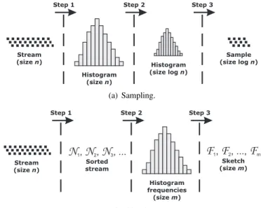
Step 1: Build a histogram of the sensor stream.

Step 2: Create a sample based on the histogram obtained in Step 1. To create such a sample, we randomly choose the elements of each histogram class, respecting the sample size and the class frequencies of the histogram. Thus, the resulting sample will be represented by the same histogram.

Step 3: Sort the data sample according to its order in the original data.

These steps are illustrated in Fig. 1(a). The original sensor stream is composed ofnelements. The histogram of the sensor streaming is built in Step 1. A minor histogram is built in Step 2, which has the sample size required (in this caselogn), and keeps the same frequencies of original histogram. Finally, the minor built histogram is reordered to keep the data sequence in Step 3.

Stream (sizen)

Histogram (sizen)

Histogram (size logn)

Sample (size logn)

Step 1 Step 2 Step 3

(a) Sampling.

Stream (sizen)

Histogram frequencies (sizem)

Step 1 Step 2 Step 3

N

₁,

N N

₂, ₃, ...

Sorted stream

F F

₁, ₂, ...,

F

_m Sketch (sizem)

(b) Sketch.

Fig. 1. Example of algorithms execution.

The pseudo-code of the sampling algorithm is given in Fig. 2. We also considern as the number of elements in the original data stream, and mas the adopted sample size.

Analyzing the algorithm in Fig. 2 we have:

• Line 1 executes inO(nlogn).

• Lines 8–13 define the inner loop that determines the

num-ber of elements at each histogram class of the resulting sample, which takesO(m)steps.

• Lines 5–18 define the outer loop in which the input data

is read and the sample elements are chosen. Because the inner loop is executed only when condition in line 6 is satisfied, the overall complexity of the outer loop is O(n) + O(m) = O(n + m) since we have an interleaved execution. ConsidernumClassthe number of histogram classes,colOrigi andcolSamplei, respectively,

the columns in original and sampled histograms, where

0 < i ≤ numClass. Basically, before evaluating the

Require:

Vector dataIn; {original data stream}

m; {sample size}

Ensure: dataOut; {sample stream} 1: Sort dataIn;

2: histScale ←“Class width”; 3: first ← dataIn[0];

4: count←0, j←0; 5: fori←0tondo

6: if (dataIn[i]>first + histScale)or(i=n−1)then 7: colFreq← ⌈m×count/dataInSize⌉;

8: while colFreq>0 do

9: index←“random element in the histogram class”; 10: dataOut[j]← dataIn[index];

11: j←j+ 1;

12: colFreq←colFreq −1; 13: end while

14: count←0; 15: first ← dataIn[i]; 16: end if

17: count←count+ 1; 18: end for

19: Re-sort dataOut; {according to the original order}

Fig. 2. Pseudo-code of the sampling algorithm.

condition of line 6,colOrigi is counted andn/numClass

interactions are executed. Whenever this condition is sat-isfied, colSamplei is built and m/numClass interactions

are executed (loop 8–13). In order to build the complete histogram, we must cover all classes (numClass), then we havenumClass( n+m

numClass) =n+m. • Line 19 re-sorts the sample in O(mlogm).

Thus, the overall complexity is O(nlogn) +O(n+m) +

O(mlogm) = O(nlogn), since m ≤ n. The space com-plexity is O(n+m) = O(n) because we store the original data stream and the resulting sample. Since every source node sends its sample stream towards the sink, the communication complexity isO(mD), whereD is the largest route (in hops) in the network.

B. Sketch-Based Algorithm

This solution is also motivated by the problem stated in Section II. Thedata reduction, can be provided by a sketch of the original data. This solution aims to keep the frequency of the data values without losses, by using a constant packet size. With this information, the data can be generated artificially in the sink node. However, the sketch solution looses the sequence of the sensor stream. The sketch algorithm can be divided into the following steps:

Step 1: Order the data and identify the minimum and maximum values in the sensor stream.

Step 2: Build the data out, only with the histogram frequen-cies.

Step 3: Mount the sketch stream, with the data out and the information about the histogram.

(4)

The execution of algorithm is presented in Fig. 1(b). The original sensor stream is composed ofnelements. The sensor stream is sorted, and the sketch information is acquired in Step 1. The histogram frequencies are built in Step 2, where mis the number of columns in the histogram. The sketch stream, with the frequencies and sketch information, is created in Step 3.

The pseudo-code of the algorithm is given in Fig. 3. We also considernas the number of elements in the original data stream, andmas the histogram column number.

Require:

Vector dataIn; {original data stream}

m; {sketch size}

Ensure: dataOut; {sketch stream} 1: Sort dataIn;

2: histScale←“Class width”; 3: first← dataIn[0];

4: m←( dataIn[n]- dataIn[0]) /histScale; 5: count←0,j←0,index←0;

6: fori←0 tondo

7: if(dataIn[i]>first +histScale)or (i=n−1)then 8: dataOut[index]←count;

9: index←index + 1; 10: count← 0; 11: first← dataIn[i]; 12: end if

13: count← count+ 1; 14: end for

Fig. 3. Pseudo-code of the sketch algorithm.

Analyzing the algorithm in Fig. 3 we have:

• Line 1 executes inO(nlogn).

• Lines 6–14 execute inO(n).

Thus, the overall time complexity isO(nlogn) +O(n) =

O(nlogn). The space complexity isO(n+m) =O(n)if we store the original data stream and the resulting sketch. Since every source node sends its sketch stream towards the sink, the communication complexity isO(mD), whereDis the largest route (in hops) in the network.

IV. EVALUATION

When we apply solutions based on data stream in a WSN, we have to analyze the network and data quality behavior. That is, what is the impact on the network, when we apply our solutions? And, how much does the application data loose when we use our solutions? These questions are answered in the following.

A. Methodology

The evaluation of the algorithms is based on the following assumptions:

• Simulation:We perform our evaluation through

simula-tions and use the NS-2 (Network Simulator 2) version 2.29. Each simulated scenario was executed with 33

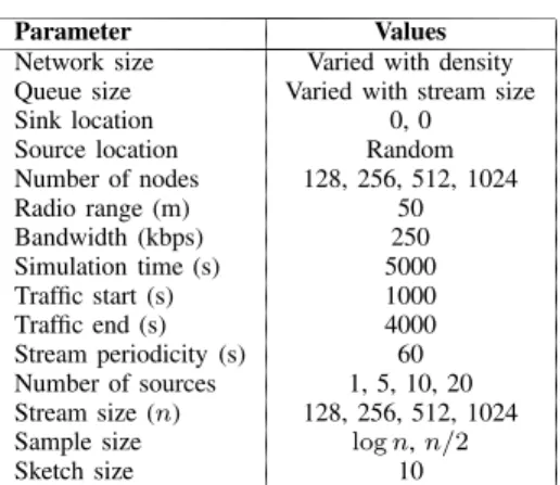
TABLE I SIMULATION PARAMETERS.

Parameter Values

Network size Varied with density Queue size Varied with stream size

Sink location 0, 0

Source location Random Number of nodes 128, 256, 512, 1024

Radio range (m) 50

Bandwidth (kbps) 250 Simulation time (s) 5000 Traffic start (s) 1000 Traffic end (s) 4000 Stream periodicity (s) 60 Number of sources 1, 5, 10, 20 Stream size (n) 128, 256, 512, 1024 Sample size logn,n/2

Sketch size 10

random topologies. At the end, for each scenario we plot the average value with 95% of confidence interval.

• Network topology: We use a tree-based routing

algo-rithm called EF-Tree [31] as the routing protocol, the density is kept constant, and all nodes have the same hardware configuration. To analyze only the application, the tree is built just once before the traffic starts.

• Stream generation: The streams used by the nodes are

always the same, following a normal distribution, where the values are between [0.0; 1.0], and the generation periodicity is 60s. The size of the data packet is 20 bytes. For larger samples, these packets are fragmented by the sources and re-assembled at the reception.

• Evaluated parameters and stream size:We varied the

number of nodes, stream size, and number of nodes generating data. In the sampling case, for each evalu-ated parameter we analyzed the application and network behavior by using sample sizes ofn/2andlogn. All pa-rameters used in the simulations are presented in Table I.

We evaluated the algorithms by considering two parts: evaluation of network behavior using the sampling and sketch solutions and evaluation of data quality using only the sampling solution. In order to evaluate the distribution approximation between the original and sampled streams, we use the Kolmogorov-Smirnov test (K-S test) [32]. This test evaluates if two samples have similar distributions, and it is not restricted to samples following a normal distribu-tion. Moreover, as the K-S test only identifies if the sam-ple distributions are similar, it is also important to evaluate the discrepancy of the values in the sampled streams, i.e., if they still represent the original stream. To quantify this discrepancy (Data Error) we compute the absolute value of the largest distance between the average of the original data and the lower or higher confidence interval values (95%) of the sampled data average, Data Error =Max{|lowervalue−

Generateavg|,|highervalue − Generateavg|}, where the pair

(lowervalue;highervalue) is the confidence interval of data

sample andGenerateavg is the average of original data.

(5)

B. Network Behavior

This evaluation considers the energy consumption of the entire network and the average delay to delivery a data packet to the sink. Another analyzed metric, not shown here, was the packet delivery ratio, and in all cases it was around100% of delivered data. In this evaluation, for the sampling algorithm, we use different sample sizes (lognandn/2) and the complete sensor stream (n), whereas for the sketch algorithm we use a fixed size (10 ranges). Both cases are analyzed with different network scenarios by varying the network size, amount of generated data at the source, and number of sources.

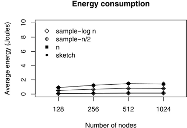
Figs. 4–6 show the energy consumption. We observe in all cases for the sampling solution that whenever the sample size is diminished the consumed energy diminishes accordingly. The sketch solution follows the sample-logn result. This occurs because the packet size is constant and close to the sample, i.e., a lognpacket size.

Analyzing separately, when the number of nodes varies (Fig. 4), the energy consumption does not vary. This occurs because only one source is used, and both the size of the sensor stream and the network density did not change. In this scenario, the sample (logn) and sketch solutions have less impact over the energy consumption.

When the size of the sensor stream varies (Fig. 5), we can observe the impact of our solutions in the energy consumption. The sample oflognand the sketch have their best performance in all cases, and the energy consumption does not vary when the sample size increases. In the sample of logn, this occurs because the packet size is increased only when we increase the sensor stream size (256, 512, 1024, 2048). In the sketch case the used packet size is always constant. The other results (samples of n/2 and n) have a worse performance because the packet size is increased proportionally when the sensor streaming size is increased.

When the number of nodes generating data varies (Fig. 6), the sample oflognand the sketch have the best performance for all cases. This occurs because, in this scenario, more packets are passing through the network when we increase the number of nodes generating data. Each source using the sample oflognor the sketch solution uses only one packet (the packet size is not more than 20 bytes) to send its data to the sink. For the other results (samples ofn/2andn) each source node generates more than one application packet, overloading the network, and causing more energy consumption.

The delay performance is given in Figs. 7–9. As for the energy results, we can see that when the sample size decreases, the delay decreases for the same reason. Again, the same effect of the number of node variation is observed (Fig. 7). When the sensor stream size and number of nodes generating data vary we can observe the impact on the delay by using our solution. Again, in the all cases, the sample of logn and sketch have the best performance.

C. Data Quality

Here, we present the impact of our solution by evaluating the data quality. This evaluation is only for the sampling so-lution, because this solution looses information in its process,

Energy consumption

Number of nodes

Average energy (Joules)

sample−log n sample−n/2 n sketch

128 256 512 1024

02468

1

0

Fig. 4. Total energy consumption with different network sizes.

Amount of data generated at the source node

256 512 1024 2048

02468

1

0

Fig. 5. Total energy consumption with different stream sizes.

Number of nodes genarating data

1 5 10 20

02468

1

0

Fig. 6. Total energy consumption with different number of sources.

and, therefore it is important to evaluate its impact on the data quality. In the sketch case, all data can be generated artificially when it arrives in the sink node, and, therefore the looses are not identified when the data tests are applied. The only impact generated by the sketch solution is the lost of the data sequence, which is not evaluated in this work.

Again, the impact of the sampling solution is made through the K-S test and the average error. Like the network evaluation,

(6)

Packet delay

Number of nodes

Average delay (seconds)

128 256 512 1024

012345

Fig. 7. Average delay with different network sizes.

Packet delay

256 512 1024 2048

012345

Fig. 8. Average delay with different stream sizes.

Packet delay

1 5 10 20

012345

Fig. 9. Average delay with different number of sources.

we use different sample sizes (lognandn/2) and the complete sensor stream (n) in different network scenarios. We vary the network size, the amount of data generated at the source, and the number of sources.

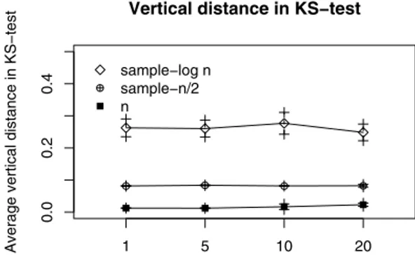
Figs. 10–12 show the similarity between the original and sampled stream distributions. The difference between them is called ks-diff. The results show that when the sample size is decreased the ks-diff increases. Because the data streams are

generated between [0.0; 1.0],ks-diff = 20%forlognsample sizes, and ks-diff = 10% forn/2 sample sizes. In all cases, the error is constant, since the data lost is small. The greater error occurs when we use a minor sample size but the data similarity is kept.

Vertical distance in KS−test

Number of nodes

Average vertical distance in KS−test

sample−log n sample−n/2 n

128 256 512 1024

0.0

0.2

0.4

Fig. 10. K-S distance in different network sizes.

256 512 1024 2048

0.0

0.2

0.4

Fig. 11. K-S distance with different stream sizes.

1 5 10 20

0.0

0.2

0.4

Fig. 12. K-S distance with different number of sources.

We also evaluate the data quality through the discrepancy between the original and sampled stream average values

(7)

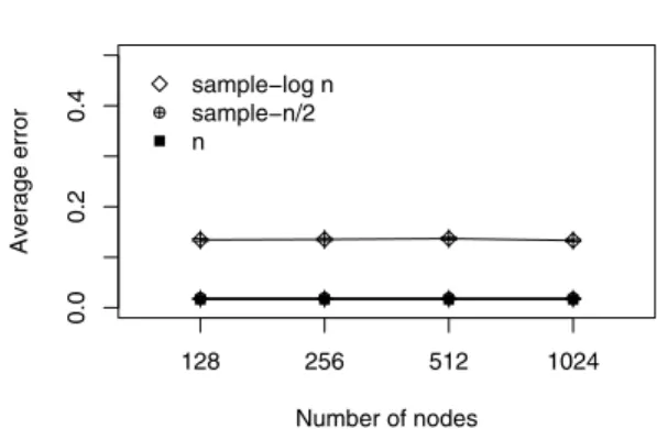
(Figs. 13–15). This error we call data-error. Like theks-diff, when the sample size is decreased, the data-errorincreases. However, data-error = 10%for samples of logn, and data-erroris almost zero for samples ofn/2. Again, in all cases the error is constant for the same reason of the ks-diff. However an important observation is that the data-error is the same for samples of n/2 andn. Therefore, if we want to keep the maximum data quality, considering the data-error, we must send only samples of n/2.

Data error

Number of nodes

Average error

128 256 512 1024

0.0

0.2

0.4

Fig. 13. Average error with different network sizes.

Data error

Average error

256 512 1024 2048

0.0

0.2

0.4

Fig. 14. Average error with different stream sizes.

D. Results Summary

In summary, when we analyze the data quality against the network behavior, we have the following conclusions:

• The sketch reduces the energy consumption and delay

by keeping a constant transmitted data rate. Once, the data rate can be generated artificially in the sink, the data quality is not affected in the distribution similarity and average discrepancy. The problem is the sequence of data lost. But the sequence lost may be acceptable by a large majority of applications when the network restrictions are strong. The cases where the data sequence is important we must use the sampling solution.

Data error

Average error

1 5 10 20

0.0

0.2

0.4

Fig. 15. Average error with different number of sources.

• The sample oflognreduces the energy consumption and

delay by reducing the transmitted data. However, the data quality is affected in the distribution similarity (20%) and average discrepancy (10%). But this quality may be acceptable by a large majority of applications when the network restrictions are strong.

• The sample ofn/2 is interesting either when the

appli-cation priority is the average discrepancy (near zero), or we have the scenario presented in Fig. 4, in which the stream size and number of nodes generating data do not vary.

• It is not interesting to use our algorithm (sample of n)

when we have to keep the same data quality similarity and we do not have to worry about the WSN restrictions.

• Finally there is the question of using sampling or sketch.

If the data sequence is important we should use the sampling algorithm. In this case we can always analyze the application and network requirements to decide about the best sample size. If the sequence is not important we can use the sketch because it always has the best network performance keeping the integrity of all data. The advantage of the sketch over sampling is that the former solution can be modified for on-line processing of the sensor stream, without keeping the original data. Finally, our solution can be applied to the problem addressed in Section II, and the results answer the questionsData quality, Data reduction, andLosses vs. benefitspresented in Section II.

V. CONCLUSION ANDFUTUREWORK

WSNs are energy constrained, and the extension of their lifetime is one of the most important issues in the design of such networks. Usually, these networks collect a large amount of data from the environment. In contrast to the conventional remote sensing — based on satellites that collect large images, sound files, or specific scientific data — sensor networks tend to generate a large amount of sequential small and tuple-oriented data from several nodes, which constitutes data streams.

In this work, we proposed and evaluated two algorithms based on data stream that use sampling and sketch techniques

(8)

to reduce data traffic and, consequently, decrease the delay and energy consumption. This work represents a way of dealing with energy and time constraints at the application level, as a complementary view of solutions that deal with this problem in the lower network levels.

The results show the efficiency of the proposed methods by extending the network lifetime — since data transmission demands lots of energy — and by reducing the delay without loosing data representativeness. Such a technique can be very useful to design energy-efficient and time-constrained sensor networks if the application is not so dependent on the data precision or the network operates in an exception situation (e.g., there are few resources remaining or there is an urgent situation).

As future work, we intend to apply the proposed method to process sensor streams along the routing task and in clustered networks. Thus, not only the data from a source can be reduced, but similar data from different sources can also be reduced, resulting in more energy efficiency. We also intend to evaluate other solutions like wavelets where specifically data characteristics can be analyzed. However, we plan to use other data distributions to analyze the behavior of our algorithms and use other scenarios when data losses can affect the data quality.

REFERENCES

[1] D. Estrin, R. Govindan, J. Heidemann, and S. Kumar, “Next century challenges: Scalable coordination in sensor networks,” inFifth Annual International Conference on Mobile Computing and Networks (Mobi-Com’99). Seattle, Washington, USA: ACM Press, August 1999, pp. 263–270.

[2] I. F. Akyildiz, W. Su, Y. Sankarasubramaniam, and E. Cayirci, “A survey on sensor networks,”IEEE Communications Magazine, vol. 40, no. 8, pp. 102–114, August 2002.

[3] T. Arampatzis, J. Lygeros, and S. Manesis, “A survey of applications of wireless sensors and wireless sensor networks,” in Mediterranean Control Conference (Med05), 2005.

[4] E. Elnahrawy, “Research directions in sensor data streams: Solutions and challenges,” Rutgers University, Tech. Rep. DCIS-TR-527, May 2003. [5] M. Datar, A. Gionis, P. Indyk, and R. Motwani, “Maintaining stream

statistics over sliding windows,”SIAM Journal on Computing, vol. 31, no. 6, pp. 1794–1813, 2002.

[6] M. R. Henzinger, P. Raqhavan, and S. Rajagopalan, “Computing on data stream,” Digital Systems Research Center, Tech. Rep., May 1998. [7] S. Muthukrishnan, “Data streams: Algorithms and applications,” in4th

ACM-SIAM Symposium on Discrete algorithms, Baltimore, Maryland, 2003.

[8] Z. Bar-Yosseff, R. Kumar, and D. Sivakumar, “Reductions in streaming algorithms, with an application to counting triangles in graphs,” in13th Annual ACM-SIAM Symposium on Discrete algorithms (SODA’02). San Francisco, California, USA: ACM SIAM, January 6–8 2002, pp. 623– 632.

[9] L. S. Buriol, D. Donato, S. Leonardi, and T. Matzner, “Using data stream algorithms for computing properties of large graphs,” inWorkshop on Massive Geometric Data Sets (MASSIVE’05), Pisa, Italy, June 9 2005. [10] M. Charikar, K. Chen, and M. Farach-Colton, “Finding frequent items in data streams,” inLecture Notes In Computer Science. Proceedings of the 29th International Colloquium on Automata, Languages and Programming, vol. 2380. Springer–Verlag, July 2002, pp. 693–703. [11] M. Datar and S. Muthukrishnan, “Estimating rarity and similarity

over data stream windows,” in Lecture Notes In Computer Science. Proceedings of the 10th Annual European Symposium on Algorithms, September 2002, pp. 323–334.

[12] P. Indyk, “A small approximately min–wise independent family of hash functions,” in 10th Annual ACM-SIAM Symposium on Discrete Algorithms (SODA’99). Baltimore, Maryland, United States: ACM– SIAM, January 17–19 1999, pp. 454–456.

[13] J. Zhao, “An implementation of min-wise independent permutation family,” http://www.icsi.berkeley.edu/∼zhao/minwise/, May 2006. [14] A. Z. Broder, M. Charikar, A. M. Frieze, and M. Mitzenmacher, “Min–

wise independent permutations,”Computer and System Sciences, vol. 60, pp. 630–659, October 2000.

[15] A. Lins, E. F. Nakamura, A. A. Loureiro, and C. J. Coelho Jr., “Beanwatcher: A tool to generate multimedia monitoring applications for wireless sensor networks,” inManagement of Multimedia Networks and Services, ser. Lecture Notes in Computer Science, A. Marshall and N. Agoulmine, Eds., vol. 2839. Belfast, Northern Ireland: Springer-Verlag Heidelberg, September 2003, pp. 128–141.

[16] ——, “Generating monitoring applications for wireless networks,” in

Proceedings of the 9th IEEE International Conference on Emerging Technologies and Factory Automation (ETFA 2003), Lisbon, Portugal, September 2003.

[17] D. J. Abadi, W. Lindner, S. Madden, and J. Schuler, “An integration framework for sensor networks and data stream management systems,” inProceedings of the Thirtieth International Conference on Very Large Data Bases. VLDB 2004, September 2004, pp. 1361–1364.

[18] B. Babcock, S. Babu, M. Datar, R. Motwani, and J. Widom, “Models and issues in data stream systems,” inProceedings of the twenty–first ACM SIGMOD–SIGACT–SIGART symposium on Principles of database systems, June 2002, pp. 1–16.

[19] S. R. Madden, M. J. Franklin, J. M. Hellerstein, and W. Hong, “Tinydb: An acquisitional query processing system for sensor networks,” ACM Transactions on Database Systems (TODS), vol. 30, no. 1, pp. 122–173, March 2005.

[20] Y. Yao and J. Gehrke, “Query processing for sensor networks,” inFirst Conf. on Innovative Data Systems Research (CIDR), January 2003. [21] S. Babu, L. Subramanian, and J. Widom, “A data stream management

system for network traffic management,” inProceedings of Workshop on Network-Related Data Management (NRDM’01). Santa Barbara, California, USA: ACM SIGMOD, May 25 2001, p. n. 2.

[22] J. Ledlie, C. Ng, D. A. Holland, K.-K. Muniswamy-Reddy, U. Braun, and M. Seltzer, “Provenance–aware sensor data storage,” in 1st IEEE International Workshop on Networking Meets Databases (NetDB), April 2005.

[23] Y. E. Ioannidis and V. Poosala, “Histogram-based approximation of set-valued query answers,” in Proceedings of the 25th VLDB Conference, Edinburgh, Scotland, 1999.

[24] D. Ganesan, S. Ratnasamy, H. Wang, and D. Estrin, “Coping with ir-regular spatio-temporal sampling in sensor networks,”ACM SIGCOMM Computer Communication Review, vol. 34, no. Issue 1, pp. 125–130, January 2004.

[25] R. Willett, A. Martin, and R. Nowak, “Backcasting: adaptive sampling for sensor networks,” inProceedings of the third international sympo-sium on Information processing in sensor networks, ACM. Berkeley, California, USA: ACM Press. New York, NY, USA, April 2004, pp. 124–133.

[26] A. Jain and E. Y. Chang, “Adaptive sampling for sensor networks,” in

Proceeedings of the 1st international workshop on Data management for sensor networks: in conjunction with VLDB 2004, vol. 72, ACM. Toronto, Canada: ACM Press. New York, NY, USA, August 2004, pp. 10–16.

[27] A. D. Marbini and L. E. Sacks, “Adaptive sampling mechanisms in sensor networks,” inLondon Communications Symposium - LCS2003, London, UK, September 2003.

[28] K. R. Silvia Santini, “An adaptive strategy for quality-based data reduction in wireless sensor networks,” in3rd International Conference on Networked Sensing Systems (INSS 2006), Chicago, USA, 31 May – 2 June 2006.

[29] P. von Rickenbach and R. Wattenhofer, “Gathering correlated data in sensor networks,” in Proceedings of the 2004 joint workshop on Foundations of mobile computing. Philadelphia, PA, USA: ACM Press New York, NY, USA, October 2004, pp. 60–66.

[30] J. Zhu and S. Papavassiliou, “A resource adaptive information gathering approach in sensor networks,” in Sarnoff Symposium on Advances in Wired and Wireless Communication, 2004 IEEE. Nassau Inn in Princeton, NJ, USA: IEEE, April 2004, pp. 115–118.

[31] E. F. Nakamura, F. G. Nakamura, C. M. Figueredo, and A. A. Loureiro, “Using information fusion to assist data dissemination in wireless sensor networks,”Telecommunication Systems, vol. 30, no. 1-3, pp. 237–254, November 2005.

[32] S. Siegel and J. N. John Castellan, Nonparametric Statistics for the Behavioral Sciences, 2nd ed. McGraw-Hill College, January 1988.