www.the-cryosphere.net/5/791/2011/ doi:10.5194/tc-5-791-2011
© Author(s) 2011. CC Attribution 3.0 License.
The Cryosphere
Deriving mass balance and calving variations from reanalysis data
and sparse observations, Glaciar San Rafael, northern Patagonia,
1950–2005
M. Koppes1, H. Conway2, L. A. Rasmussen2, and M. Chernos1
1Department of Geography, University of British Columbia, 1984 West Mall, Vancouver, BC V6T 1Z2, Canada 2Department Earth & Space Sciences, University of Washington, Box 351310, Seattle, WA 98195-1310, USA Received: 29 March 2011 – Published in The Cryosphere Discuss.: 14 April 2011
Revised: 14 September 2011 – Accepted: 17 September 2011 – Published: 29 September 2011
Abstract.Mass balance variations of Glaciar San Rafael, the northernmost tidewater glacier in the Southern Hemisphere, are reconstructed over the period 1950–2005 using NCEP-NCAR reanalysis climate data together with sparse, local historical observations of air temperature, precipitation, ac-cumulation, ablation, thinning, calving, and glacier retreat. The combined observations over the past 50 yr indicate that Glaciar San Rafael has thinned and retreated since 1959, with a total mass loss of∼22 km3of ice eq. Over that period, ex-cept for a short period of cooling from 1998–2003, the cli-mate has become progressively warmer and drier, which has resulted primarily in pervasive thinning of the glacier surface and a decrease in calving rates, with only minor acceleration in retreat of the terminus. A comparison of calving fluxes derived from the mass balance variations and from theoret-ical calving and sliding laws suggests that calving rates are inversely correlated with retreat rates, and that terminus ge-ometry is more important than balance fluxes to the termi-nus in driving calving dynamics. For Glaciar San Rafael, regional climate warming has not yet resulted in the signifi-cant changes in glacier length seen in other calving glaciers in the region, emphasizing the complex dynamics between climate inputs, topographic constraints and glacier response in calving glacier systems.
Correspondence to:M. Koppes ([email protected])
1 Introduction
Recent observations from Patagonia indicate widespread thinning and retreat of the outlet glaciers that drain the Patag-onian Icefields (Rignot et al., 2003; Rivera et al., 2007), one of the last remaining large reserves of ice outside of the polar regions (Dyurgerov and Meier, 1997). This retreat is likely caused in part by regional warming of∼0.5◦C over the past 40 yr (Rasmussen et al., 2007). Many of these outlet glaciers terminate in fjords or lakes, and their response to climate is complicated by their sensitivity to non-climatic influences such as terminus geometry, sediment delivery to the termi-nus, ice-front melt rates, and water depth (Meier and Post, 1987; Powell, 1991; van der Veen, 1996; Warren and Aniya, 1999; Motyka et al., 2003; O’Neel et al., 2005; Pfeffer, 2007; Rignot et al., 2010). Hence, retreat histories of such tidewater glaciers contain a record both of past climate and of changing ice-front dynamics.
understand how these cooler, more arid conditions may have affected the mass balance of the icefields, a closer look at the response of these outlet glaciers to recent climatic changes is needed.
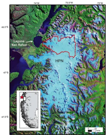
In this study we use a glacier mass balance model and NCEP-NCAR reanalysis data (Kalnay et al., 1996; Kistler et al., 2001), constrained by sparse observations of local climate and glacier change to reconstruct the mass balance variations of Glaciar San Rafael, the only tidewater glacier that drains the Northern Patagonian Icefield. The icefield, also known as the Hielo Patagonico Norte (HPN – Fig. 1) extends from approx. 46.5◦ to 47.5◦S, covering an area of ∼4200 km2, and the highest peak, Monte San Valentin, rises to 3910 m. Of the 41 glaciers draining the HPN, 20 of them end in freshwater lakes or fjords. San Rafael is the only glacier in the HPN that calves into seawater; it is also the lowest latitude ocean-terminating glacier in the world. Our primary goal in reconstructing the mass balance history of Glaciar San Rafael is to document ongoing glacier and cli-mate changes in Patagonia, one of the largest and most sen-sitive remaining areas of temperate ice and a potentially sig-nificant contributor to sea level rise (Rignot et al., 2003); it is also a region where little attention has been paid to glacier mass balance changes prior to the advent of cryospheric re-mote sensing in the late 20th century. Our secondary goal is to demonstrate how sparse glacier observations can be used to constrain a glacier mass balance history, based on global climate reanalysis data, in regions where the local and re-gional climate history is not well documented, in order to understand how the glacier response to recent (50 yr) climate conditions might pertain to both earlier glacial conditions and future climatic change in the region. A further goal is to com-pare our observation-driven model results to a suite of calv-ing “laws” to help interpret the dominant drivers of tidewater calving.
2 Regional climate history
The HPN is located in the “roaring Forties”, a region charac-terized by a cool, wet climate throughout the year, with fre-quent precipitation-bearing storms. Ice cover in the region is sustained by this extreme precipitation; Escobar et al. (1992) estimated present-day annual precipitation of 6.7 m water equivalent averaged over the broad plateau of the HPN. Sea-sonal variations in precipitation and temperature are small; summers are wet and windy (Fujiyoshi et al., 1987) and pre-cipitation can fall as snow year-round (Kondo and Yamada, 1988). Although seasonal variations are small, interannual variations in precipitation can be large (Enomoto and Naka-jima, 1985); Warren and Sugden (1993) suggested that these large interannual variations in precipitation exert a strong control on glacier dynamics. They also noted that decadal mean temperature and precipitation are positively correlated; when the climate is warmer, it is also wetter.
Fig. 1. Location of Glaciar San Rafael in the Campo de Hielo Patagonico Norte (HPN), Chile. Solid-line marks map extent of the glacier; dashed-line indicates present-day equilibrium line (about 1300 m a.s.l.). The glacier calves into Laguna San Rafael (LSR), which is connected to ocean waters through the Rio Tempano. The star shown in the inset map is the location of the NCEP-NCAR grid point SR1 at 46.67◦S, 75◦W.
3 Glacier observations
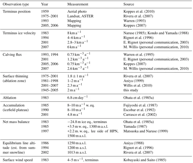
Table 1.Summary of all climate, mass balance, surface and terminus observations made on or near San Rafael Glacier, 1950–2005.
Observation type Year Measurement Source
Terminus position 1959 1975–2001 1993 2005, 2006
Aerial photo Landsat, ASTER Mapping Mapping
Koppes et al. (2010) Rivera et al. (2007) Warren (1993) Koppes (2007)
Terminus ice velocity 1983 1994 2001 2007
8 km a−1 4–6 km a−1 2.8–3 km a−1 6 km a−1
Naruse (1985); Kondo and Yamada (1988) Rignot et al. (1996)
E. Rignot (personal communication, 2003) M. Willis (personal communication, 2010)
Calving flux 1993, 1994
2001 2005, 2006 2007
0.73 km−3a−1 1.2 km−3a−1 0.75 km−3a−1 2.6 km−3a−1
Warren et al. (1995)
E. Rignot (personal communication, 2003) Koppes (2007)
M. Willis (personal communication, 2010)
Surface thinning (ablation zone)
1975–2001 1981–1998 2001–2007 1945–2005
1.8±1 m a−1 1–2 m a−1 2.3 m a−1 2 m a−1
Rivera et al. (2007) Aniya (1999) Willis et al. (2010) this study
Ablation 1983 6.8 cm day−1 Ohata et al. (1985a)
Accumulation (icefield plateau)
1985 1990 2001
8–10 m a−1w. eq. 8–10 m a−1 4.8 m a−1
Fujiyoshi et al. (1987) Escobar et al. (1992) Carrasco et al. (2002)
Net mass balance 1983 1985 1997
−24.8 m ice eq., terminus +3.5 m w. eq., 1300 m a.s.l. +2.2 m. w. eq., lee side of HPN, 1500 m a.s.l.
Ohata et al. (1985a) Yamada (1987)
Matsuoka and Naruse (1999)
Equilibrium line alti-tude (est. from sum-mer snowline)
1986 1994 2002
1250 m a.s.l. 1200 m a.s.l. 1013 m a.s.l.
Aniya (1988) Rignot et al. (1996) Rivera et al. (2007)
Surface wind speed 1983 4–5 m s−1, terminus Kobayaski and Saito (1985)
end of the Little Ice Age, which terminated approx. 1900 AD (Araneda et al., 2007; Koppes et al., 2010).
3.1 Surface geometry and topography
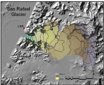
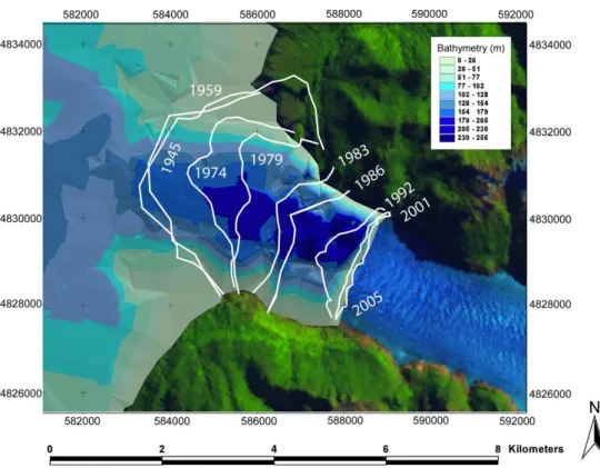
We used data from the Shuttle Radar Topography Mission in 2000 (SRTM-2000) to construct a digital elevation model (DEM) of Glaciar San Rafael (Fig. 2). We also mapped the bathymetry of Laguna San Rafael using ship-board sonar in 2005 and 2006 (Koppes, 2007; Koppes et al., 2010) (Fig. 3) to construct the submarine terminus cross-sectional area. Analysis of the glacier DEM, which has horizontal resolution of∼50 m, indicates that the present-day area of the glacier is 728 km2(Fig. 2); it drains∼19 % of the HPN icefield. Al-most 40 % of the surface area of the glacier lies within the “ELA zone”, between∼1075–1460 m, as modeled from the reanalysis data (see Sect. 4.1). Figure 7 shows the current area-altitude distribution of the glacier. The ELA zone also
corresponds to the peak in orographic precipitationk(z); this is discussed further in Sect. 4.2.
3.2 Surface velocity
Fig. 2.Digital elevation model of Glaciar San Rafael obtained from SRTM-2000 data. Dashed blue line represents the mean ELA. 100-m contours are indicated in thin black lines. Measure100-ments of daily temperature and precipitation were collected at CONAF field station LSR, along the Andean rangefront.
(∼1200 m a.s.l., 17 km upglacier from the terminus). Ad-ditional InSAR measurements from Radarsat images taken in 2001 show surface velocities near the terminus decreased to 2.8–3 km a−1(E. Rignot, personal communication, 2003) and 2.6 km a−1in 2007 (M. Willis, personal communication, 2010). We note that these velocities were measured by track-ing features on the glacier surface, and hence include both longitudinal strain rates and crevasse opening rates; true ter-minus velocities could be smaller, and the ice flux delivered to the terminus calculated using these velocities would be correspondingly smaller; hence, these ice velocities repre-sent an upper bound for modeling calving rates.
3.3 Calving
Glaciar San Rafael remains an actively calving glacier; calving events from both above and below the water-line occur every few minutes. Warren et al. (1995) ob-served calving events during the summers of 1993 and 1994 and estimated that the mean summer calving flux was ∼2×10⁻³km3day−1, with an annual flux of 0.73 km3a−1, assuming that calving rates do not vary appreciably across the seasons. We are confident in such an assumption, as our observations of calving events during midwinter 2005 and again in autumn 2006 indicated similar calving fluxes of 0.75 km3a−1. Both estimates are slightly less than esti-mates from InSAR-derived velocities in 2001 and ASTER-derived velocities from 2007 near the terminus: terminus ve-locities of 2.8 km a−1in 2001 (E. Rignot, personal commu-nication, 2003), and up to 6 km a−1(Willis et al., 2010) dur-ing a two-week period in 2007, coupled with a 2001–2007
terminus ice front area of 0.42 km2derived from the lagoon bathymetry, imply that the calving flux derived from satel-lite remote sensing in 2001 was∼1.2 km3a−1, and in 2007 was up to ∼2.6 km3a−1 (M. Willis, personal communica-tion, 2010).
3.4 Retreat history
Glaciar San Rafael has been in stop-start retreat throughout the 20th century. Since 1978, the glacier has retreated into a narrowing valley that crosses the Andean range front, and the terminus has changed from an extensive piedmont lobe approx. 7 km wide, to a narrow∼2 km calving front. Fig-ure 3 shows a compilation of terminus positions that we de-rived from: (1) aerial photos taken by the Chilean and US Air Forces in 1945 and 1959; (2) Landsat and ASTER im-ages collected since 1979; (3) field observations, including a series of paint marks on the northern fjord wall that marked the yearly position of the northern edge of the calving cliff from 1983 to 2002; (4) measurements using ship-borne radar in 2005 and 2006; and (5) observations collated by War-ren (1993). Anecdotal evidence from the Chilean Park Ser-vice, as well as these observations, suggest that although Glaciar San Rafael has experienced short-term, seasonal ad-vances of the terminus, it has not experienced a multi-year re-advance at any time during the past 50 yr. Given the evi-dence, we assume that the terminus was either stable or re-treating between years in which the terminus position was mapped, and we interpolate the rate of retreat between the known locations of the terminus over time using a cubic spline (Fig. 4).
Prominent trimlines along the valley walls provide a his-tory of ice thickness change during this period. Rivera et al. (2007) compared Landsat MSS and ETM+ images from 1975 and 2001 and estimated an average thinning of the ice-field surface of 1.8±1.0 m a−1around the outer margins of the HPN (including the terminal zones and lateral margins of the ablation areas of the outlet glaciers), with most of the outlet glaciers either maintaining stable terminus positions or in slow retreat. Similar rates of thinning (1–2 m a−1)over the ablation zone of San Rafael were estimated by Aniya (1999) between 1981 and 1998 using photogrammetric methods, as well as by Willis et al. (2010; ∼2.3 m a−1)between 2001– 2007 using repeat ASTER satellite imagery. In July 2005, we measured a prominent trimline 120 m directly above the terminus ice cliff using a laser rangefinder. An early photo taken by the Chilean Air Force shows that the glacier surface was at this trimline in 1945; thinning in the vicinity of the present-day terminus has therefore averaged∼2 m a−1since 1945.
Fig. 3. Terminus positions of Glaciar San Rafael from 1945 to 2006, and bathymetry of Laguna San Rafael. The terminus was relatively stationary between 1945 and 1959, and again between 2001 and 2006. Bathymetry was mapped using ship-board sonar in 2005 and 2006.
Fig. 4. History of the ice-front areaAterm (grey line) calculated from the bathymetry of Laguna San Rafael, known terminus posi-tions (black dots), and interpolated terminus posiposi-tions (black line) (see Fig. 3). For the calculation of changes inAtermover time we assume that, on average, the cliff height across the terminus was 40 m above the water line.
water depths decreasing to∼140 m on either side of a narrow central trough; the 2005 area of the terminus Aterm above and below the waterline is 0.42 km2 (Fig. 4). We estimate the annual history of the terminus areaAtermfrom 1950 to
2005 using the interpolated terminus locations and our new high resolution map of the bathymetry of Laguna San Rafael (Fig. 3), assuming that the average ice cliff height of 40 m above water line did not change appreciably during this time. Results in Fig. 4 show a marked change in terminus area (and sharp decrease in the annual rate of retreat) when the calving front retreated into the narrowing valley in the early 1980s.
3.5 Ablation
Measurements by Ohata et al. (1985a, b) from a network of 17 stakes set along a transect extending from near the termi-nus of Glaciar San Rafael up to 1050 m a.s.l. indicated that the average rate of ablation near the terminus during Decem-ber 1983 was 6.8 cm day−1in ice eq., with daily-average ice ablation decreasing with elevation at a rate of 6 cm km−1. We use concurrent temperature measurements made at La-guna San Rafael in December 1983 by Enomoto and Naka-jima (1985), together with temperature lapse rate profiles T (z)from the NCEP-NCAR data for the same time period (Sect. 4.1), to establish a relationship between daily-average ablation ˙a(z)temperature T (z), considering only T (z) >0 ◦C:
(Ohata et al., 1985a) and reflect ablation over a local daily mean temperature range of 5 to 13◦C. To estimate ablation of snow, we follow results of Hock (2003) for similar tem-perate glacial systems in Norway, Iceland and the Alps and assume that the positive degree-day (PDD) factor for snow is 0.6±0.1 that for ice. That is, for snow:
˙a(z)=0.39T (z) [snow] (1b)
In our mass balance model (Sect. 4.2), we track whether precipitation on the previous day fell above or below the daily snowline (where T <2◦C), and then choose either Eq. (1a) or Eq. (1b) to estimate daily ablation at (z) ac-cordingly. This is obviously a source of uncertainty in the model, as we assume that any snow that might have fallen whenT <2◦C will be ablated away if in the following days T >0◦C, and thereafter the ice ablation co-efficient will ap-ply. This will tend to overestimate the ablation rate, but only during the start of the melt season near the snowline as the snowline is rising but the model is estimating snow removal faster than may be actually be occurring.
3.6 Surface mass balance and equilibrium line altitudes
The few point measurements of annual mass balance that have been collected near San Rafael glacier range from −24.8 m ice eq. at the terminus in 1983 (Ohata et al., 1985a), +3.5 m w. eq. at an elevation of 1296 m a.s.l. on the icefield plateau during 1985 (Yamada, 1987), and +2.2 m w. eq. at an elevation of 1500 m a.s.l. on Glacier Nef on the lee (east) side of the icefield during 1997 (Matsuoka and Naruse, 1999). Al-though sparse, these observations provide useful targets for tuning both the precipation enhancement factork(z) to es-timate the accumulation profile (see Sect. 4.1, Eq. 4), and the two ablation PDD co-efficients (Eq. 1a and 1b). Equilib-rium line altitude (ELA) observations from prior studies are: 1250 m a.s.l. in 1986 (Aniya, 1988), 1200 m a.s.l. in 1994 (Rignot et al., 1996) and 1013 m a.s.l. in 2002 (Rivera et al., 2007). These provide additional constraints for tuning the mass balance model (see Sect. 4.2).
4 Glacier mass budget model
4.1 Reconstructing local surface mass balance 1950–2005
The NCEP-NCAR Reanalysis climate database is derived from historical observations of various meteorological vari-ables made at the surface, from radiosondes and from satel-lites (Kalnay et al., 1996; Kistler et al., 2001). The database consists of 6-hourly estimates of meteorological variables at standard atmospheric pressure levels on a 1.9◦ global grid extending back to January 1948. The nearest NCEP-NCAR surface gridpoint to Glaciar San Rafael, at 46.67◦S, 75◦W, is shown as a star in Fig. 1 and henceforth referred to as
SR1. Located to the west of the glacier, near the coast, grid-point SR1 was chosen to best reflect the dominant synoptic weather patterns upstream of the study area. Rasmussen et al. (2007) used the NCEP-NCAR data to show that the 850-hPa precipitation flux at 45◦S (calculated fromU850RH850 where U850 is the component of the wind from direction 270◦and RH850is the relative humidity) decreased by about 10 % over 1948–1998. However, the fraction falling as snow at 850 hPa (calculated fromU850RH850 whenT ≤2◦C) de-creased by about 20 %; hence, the combined effects of warm-ing and drywarm-ing have caused the 850-hPa snowfall at 45◦S to decrease by about 28 %.
Although we show model results from 1950 to 2005 using the NCEP-NCAR dataset, caution is needed when interpret-ing results from 1950 to 1960 because of inhomogeneities in the instrumental record in the late 1950s (see Rasmussen et al., 2007). For this reason, herein we focus our statistical and model analysis on climate and glacier changes from 1960 to 2005; however, we include the entire record available to 1950 in our model runs, with caveat above, as the terminus record suggests that the ice front was unusually stable from 1950–1959.
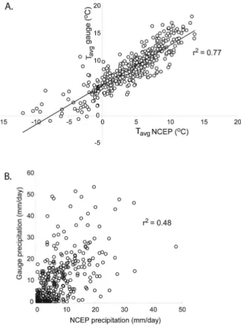
We compared the NCEP-NCAR derived climate data from SR1 with a record of 398 daily temperature and precipitation measurements that we made between March 2005 and April 2006 at a Chilean Forest Service (CONAF) guard station, lo-cated about 7 km from the glacier front on the shores of La-guna San Rafael (LSR, at 46.66◦S, 73.86◦W). We used two tipping bucket rain gauges (0.2 mm per tip) and a 2-channel temperature sensor. Air temperature (measured 1.4 m above the surface) and soil temperature (measured 2 cm below the surface) were recorded hourly. Figure 5 shows daily-average temperature and precipitation measurements at LSR, and NCEP-NCAR derived values at the 1000-hPa level at SR1. A linear regression of temperatures over the period of record yields:
TLSR=0.73TSR1+5.5
(r2=0.77;n=398;p <0.0001) (2)
whereTLSRis the daily-average air temperature (◦C) at La-guna San Rafael, andTSR1is the daily-average 2-m air tem-perature at SR1.
Fig. 5. Comparison of 398 daily-average measurements of tem-perature(a)and precipitation(b)made at Laguna San Rafael from March 2005 to April 2006, with NCEP-NCAR derived values at 2 m above ground at gridpoint SR1. Correlation co-efficients are 0.77 and 0.48, respectively.
is improved by including the zonal wind speedUSR1(m s−1) modeled at 10 m above ground to reflect the magnitude of storm intensity:
PLSR=0.78PSR1+0.9|USR1| +0.82
(r2=0.50;n=398;p <0.0001) (3)
wherePLSR andPSR1 are daily precipitation in mm at La-guna San Rafael and the NCEP-NCAR gridpoint SR1, re-spectively. We note that wind speeds measured near the ter-minus of San Rafael in 1983 were∼4–5 m s−1 (Kobayashi and Saito, 1985), while NCEP-NCAR derived winds at SR1 are typically 2–3 times stronger (10–15 m s−1)for the same period.
We calculate the uncertainties in our statistical down-scaling approach using the leave-one-out cross-validation method, wherein multiple monthly blocks of data were re-moved from the local calibration dataset (PLSR andTLSR) and a new linear regression with the NCEP-NCAR dataset (Eqs. 2, 3) was performed in order to estimate errors from the least squares regression. The regression coefficients (and
uncertainties) are determined as the means of coefficients from each repetition of the model fitting procedure in the cross-validation experiment (cf. Hofer et al., 2010). The maximum estimated uncertainties using our cross-validation scheme was ±0.7◦C forTavg and±4 mm day−1 for PLSR, respectively.
We use Eq. (2) and the NCEP-NCAR database to hind-cast daily-average temperatures at the terminus of Glaciar San Rafael from 1950 to 2005. We also use the NCEP-NCAR upper air temperatures from 1000, 925, 850, 700, and 600 hPa levels to reconstruct daily variations in the at-mospheric lapse rate at SR1. The average lapse rate over the period of record was 5.5±0.9◦C km−1, similar to lapse rates measured by Kerr and Sudgen (1994). We used the daily temperature at LSR (calculated using Eq. 2) and the daily lapse rates from SR1 to reconstructT (z)from sea level to the top of the glacier. DailyT (z)profiles are needed to partition the snow-fraction of precipitation and to estimate ablation (Sect. 3.5) over the glacier surface.
Figure 6a shows variations of mean annual temperature variations at Laguna San Rafael over the period 1950–2005, derived from the NCEP-NCAR record. Mean annual temper-atures at the glacier front varied only 1.3◦C about a mean of 8.9◦C, consistent with the strong maritime influence on the climate of the region.
We use Eq. (3) to estimate daily precipitation at Laguna San Rafael over the same period 1950–2005. Annual precip-itation there has varied by±0.60 m about a mean of 3.60 m (Fig. 6b). Precipitation, which was relatively high during the period 1960–1975, decreased by more than 13 % during the period 1976 to 2005.
To estimate daily precipitation in the form of snowfall over the surface of the glacierP (z)over the period 1950–2005, we scaledPLSR by an orographic enhancement factork(z)that varies spatially, so that:
P (z)=k(z)PLSR (4)
The enhancement factor k(z) is not well constrained; sparse observations and model results suggest that precip-itation on the plateau of the Northern Patagonian Icefield, ∼10 km upwind of the Andean crest, is 2.5 to 5 times that on the outer coast to the west of Laguna San Rafael (Fujiyoshi et al., 1987; Escobar et al., 1992; Carrasco et al., 2002); ob-servations from the Southern Alps of New Zealand, a sim-ilar north-south trending mountain belt protruding into the Southern Westerlies, also indicate that precipitation increases to a peak 20 km upwind of the divide that is 4–5 times that on the western coast (Wratt et al., 2000). To test the sensitiv-ity of the enhancement factork(z), we ran our accumulation model using a range of static values fromk=3 tok=5 at all elevationz(see Sect. 4.2).
Fig. 6.Reconstructed annual temperature(a)and precipitation(b) anomalies at Laguna San Rafael for the period 1950 to 2005. Local values were calculated using NCEP-NCAR data and the relation-ships established in Eqs. (1) and (2). Anomalies shown are differ-ences from the mean value for the period: mean annual temperature was 8.9◦C; mean annual precipitation at LSR was 3.60 m w. eq.
of the glacier surface (Smith and Barstad, 2004; Roe, 2005). Whereas the factork varies as a function of glacier surface elevation (z) in this orographic model, it is also possible to calculate it as a function of distance from the coast and rangefront(x), because the elevation of the glacier surface itself is a function of that distance (see Fig. 2). Cloud micro-physics in the model are represented by characteristic time delays for hydrometeor growth and fallout. The large-scale atmospheric flow is computed as a function of wind and tem-perature, and the amplitude and pattern of precipitation are then calculated as a function of that flow. Tunable model parameters include the horizontal wind speed (u), meteoric fallout rate (τf), conversion time (τc), moisture scale height (Hm), and moist static stability for upward convection (Nm). We tuned the orographic model so that the average precip-itation at the coast (∼1.8 m a−1) (Carrasco et al., 2002) in-creases by a factor of two to match observations at Laguna San Rafael (∼3.6 m a−1),∼20 km inland, and by a factor of
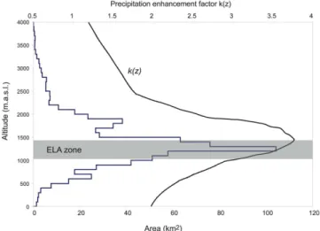
Fig. 7. Year 2000 AD area-altitude distribution of Glaciar San Rafael, in 100-m. altitude intervals, derived from SRTM data, and spatial variation in the precipitation enhancement factork(z)(black line) used to model precipitation on the glacier surface. The en-hancement factor is a multiple of precipitation at the coast. The zone of equilibrium line altitudes from 1960–2005 is indicated by the grey bar.
3.5 at 1200 m a.s.l. to match values estimated by Fujiyoshi et al. (1987) and Carrasco et al. (2002) near the equilibrium line of the glacier. The most realistic response, which produced a peak enhancement factor that best fit observations, was ob-tained with the following input parameters: u=15 m s−1, τf=τc=1000 s, Hm=3000 m, and Nm=0.005 s−1. Fig-ure 7 shows modeled spatial variations ofk(z).
4.2 Surface mass balance model
At each elevation z, the annual surface mass balance b˙(z) is the algebraic sum of accumulation˙c(z)and ablation ˙a(z) That is:
˙
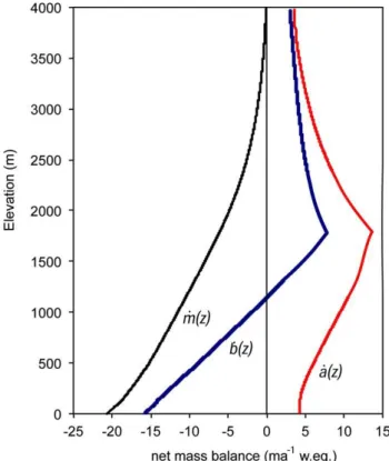
Fig. 8.Mean annual surface mass balanceb(z), accumulationc(z) and ablationa(z)derived from the mass balance model for the pe-riod 1960–2005, versus elevation. Mass balance is calculated using an orographic precipitation enhancement factork(z)from Fig. 7 and input scenario #4 (Table 2).
that the annual ELA (i.e., whereb(z)=0) ranges from 1050– 1460 m a.s.l., with a mean ELA of 1295 m a.s.l.
The concentration of orographic enhancement k(z) of snowfall around the elevation of the ELA (∼1100– 1400 m a.s.l.), as indicated by observations (Fujiyoshi et al., 1987; Escobar et al., 1992; Carrasco et al., 2002) may also be a major driver in our mass balance model. As can be seen in Fig. 8, the accumulation, and hence mass balance, gradient for this glacier shows a pronounced kink at∼1700 m a.s.l. This kink in the mass balance profile may be due in part to limited variability in temperatures in this maritime cli-mate, where the range of elevations over which the transition from solid to liquid precipitation occurs is narrow; it may also reflect the fact that a large percentage of the cumulative glacier surface area occurs in this same range of elevations. An orographically-induced peak in precipitation at the ELA would unrealistically tip the balance towards net accumula-tion if too large, or net ablaaccumula-tion if too small. As the area-elevation distribution of this glacier is so heavily weighted in a zone across the broad plateau of the icefield at the elevation of the ELA that accounts for almost 40 % of the glacier sur-face, any estimates of the cumulative balance over the past 50 yr are extremely sensitive to the location and magnitude
Fig. 9. Annual equilibrium line altitude (ELA) derived from daily snowline and the mass balance model using input scenario #4 in Ta-ble 2, from 1950–2005 (black line) and measured ELAs in 1986, 1994 and 2002 (also derived from late summer snowline) (trian-gles). Mean modeled ELA for the period 1960–2005 is 1295 m.
of an orographically-enhanced peak in precipitation in this zone.
4.3 Terminus mass budget
The fundamental equation describing fluxes near the termi-nus of calving glaciers is:
dL
dt =
Qbal+Qthin−Qcalv
Aterm (6)
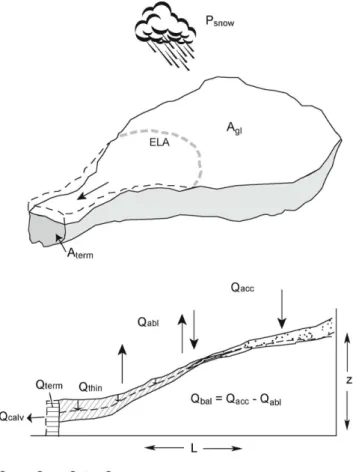
where dLdt is a change in the length of the glacier; Qbal is the surface mass balance b(z) integrated over the area of the glacier, andQthinis the volume of ice lost due to thin-ning. The flux of ice away from the terminusQcalvincludes both calving and mass loss due to submarine melting and surface ablation averaged over the area of the terminus face Aterm. A glacier is in balance when Qcalv equalsQbal, and the ice thickness and length are not changing. For a shrink-ing glacier, the ice volume decreases both through glacier shortening Qterm= −dLdtAterm and through surface lower-ingQthin= −dhdtAthin. Glacier retreat dLdt can be measured from known terminus positions andAtermcan be estimated from bathymetry, glacier thinning dhdt and the area of thin-ningAthincan be estimated from trimlines, and surface mass balanceQbal can be estimated from precipitation and tem-perature data, and so we rearrange Eq. (6) to solve explicitly for the calving fluxQcalv, which is the volume of ice passing through the terminus per unit time:
Qcalv=Qbal+Qthin+Qterm (7)
Fig. 10. Illustration of fluxes and areas relevant for estimating the mass budget of calving glaciers.
4.4 Calving model
A second means of deriving the calving flux,Qcalv, can be acquired by applying a suite of empirically and theoretically derived “calving laws” (Benn et al., 2007) using the observed bathymetry of the fjord, where former locations of the calv-ing margin are also known. In such an approach, the calvcalv-ing rate is quantified by combining the retreat ratedLdt over time with modeled terminus velocitiesUice, and then compared to ice front cross-sectional areasAtermto compute a calving flux at annual time steps. Here, the calving velocity,UD, is de-fined as the difference between the average down-glacier ice velocity at the terminus and the change in terminus position in theL-direction over time:
UD=UT−dL/dt (8)
By treating calving in this manner, quantifying the rate of ice discharge over annual timescales requires only knowl-edge of yearly terminus position and an average ice veloc-ity at the terminus. However, the controls on ice velocveloc-ity are substantial, and still poorly understood (e.g., Warren and Aniya, 1999; Benn et al., 2007). To reduce unnecessary com-plexity, for this model run we ignore longitudinal stretching
and treat glacier flow resistance as a product of lateral and basal drag.
Bathymetric transects along previous ice fronts, combined with an observed average height of the ice cliff above water-line of 40 m (H0)allows us to determine the thickness of the ice front at the terminus (HT), using a height above buoy-ancy criterion (Van der Veen, 1996), assuming the ice front is at flotation:
HT=UT− ρsw
ρi
HW+H0 (9)
whereρsw andρi are the densities of seawater and ice, re-spectively. Water depth (HW)hence is a primary control on ice front thickness at the terminus, and thinning will result in retreat until shallower water is reached. Once the ice thick-nessHTand change in the glacier surface slopeθis known, the driving stress in the downslope direction can be quanti-fied:
τD=ρigHTsinθ (10)
This driving stress is opposed by basal resistance, which can be easily altered using only a single tuning parameterC:
τB=τD
1−ρwHW ρiHT
C
(11) whereρwHWis the basal water pressure, and assuming that (a)τB=0 when the ice pressureρiHTequals the basal wa-ter pressure, and (b) τB=τD whenρwz=0. C was tuned to calibrate the calving model to observed surface velocities in 1983, 1994, and 2001 (Naruse, 1985; Rignot et al., 1996; E. Rignot, personal communication, 2003); agreement was closest whenC=0.6. This is double the value ofC corre-lated using data from Columbia Glacier (Benn et al., 2007), which could in due in part to Columbia Glacier’s more grad-ual slope (1.15◦ versus 2.67◦ at Glaciar San Rafael) (Ven-teris, 1999).
The annual velocity at the terminus was then calculated assuming a rectangular bed, using the sliding law developed in Benn et al. (2007). Mean values of basal drag, driving stress and ice thickness were used to estimate the average sliding velocityUBat the terminus:
UB= 2A n+1
1−τD−τB HT
n
Wn+1 (12)
using a flow parameterA calculated from Arrhenius’ Law andn=3 from Glen’s flow law (Nye, 1965).
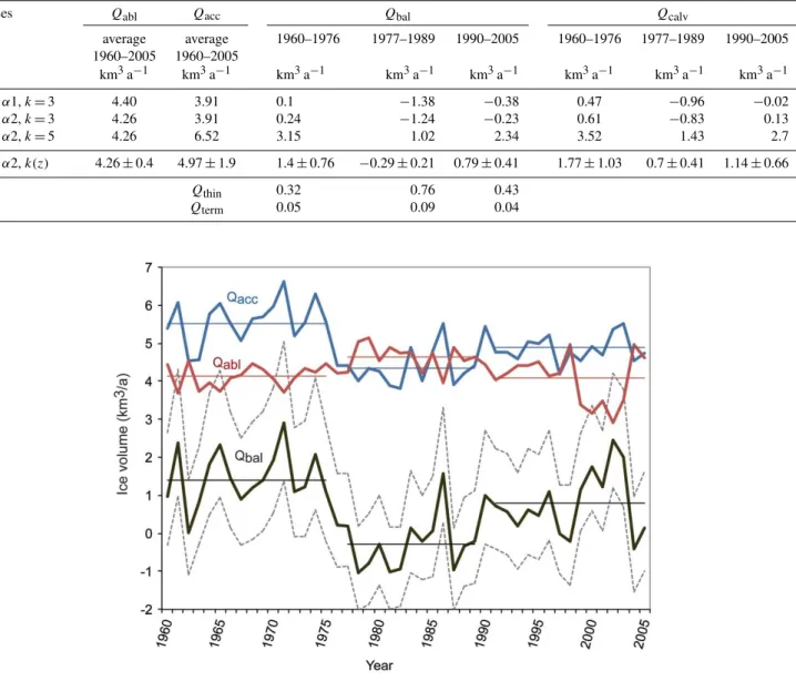
Table 2.Summary of modeled ice fluxes through Glaciar San Rafael, 1960–2005. Scenarios used in model runs: α1 = ablation flux using Eq. (1a) only;α2 = ablation flux calculated using Eqs. (1a) and (1b);k(z)= enhancement factor used in Eq. (4). Qcalvis calculated as in Eq. (7) as the sum ofQthin,QbalandQterm.QthinandQtermdid not vary from case to case.
Cases Qabl Qacc Qbal Qcalv
average average 1960–1976 1977–1989 1990–2005 1960–1976 1977–1989 1990–2005 1960–2005 1960–2005
km3a−1 km3a−1 km3a−1 km3a−1 km3a−1 km3a−1 km3a−1 km3a−1
#1:α1,k=3 4.40 3.91 0.1 −1.38 −0.38 0.47 −0.96 −0.02
#2:α2,k=3 4.26 3.91 0.24 −1.24 −0.23 0.61 −0.83 0.13
#3:α2,k=5 4.26 6.52 3.15 1.02 2.34 3.52 1.43 2.7
#4:α2,k(z) 4.26±0.4 4.97±1.9 1.4±0.76 −0.29±0.21 0.79±0.41 1.77±1.03 0.7±0.41 1.14±0.66
Qthin 0.32 0.76 0.43
Qterm 0.05 0.09 0.04
Fig. 11. Histories of annual accumulation (blue line), ablation (red line) and surface mass balanceQbal(black line) from 1960–2005. The three fluxes are derived from input scenario #4 (Table 2). The upper and lower ranges of surface mass balance fluxesQbal, derived from the various inputs cases for accumulation fluxesQaccand ablation fluxesQabllisted in Table 2, are represented by dashed grey lines. A piecewise linear fit was chosen to indicate averages during the periods 1960–1975, 1976–1990 and 1991–2005.
basal drag across the bed, allowing us to assumeUBequals the surface velocity UT (Howat et al., 2005); although we note that this approach will tend to overestimate the downs-lope ice fluxes.
5 Results
5.1 Surface mass balance
The degree-day ablation model (Eq. 1a and 1b) and pre-cipitation model (Eq. 4) were run to calculate annual ab-lation Qabl, accumulation Qacc and surface mass balance
Figure 11 shows annual accumulationQacc, ablationQabl and resultingQbal calculated over the glacier surface, and linear best fits for the periods 1960–1975, 1976–1990 and 1991–2005. Average ablation over the period 1960 to 2005 is 4.6 km3a−1. Anomalously low ablation from 1999 to 2003 was a result of anomalously low annual temperatures (see Fig. 6a). Although accumulation (snowfall) depends on the joint distribution of precipitation and temperature, the pattern of accumulation varies most closely with that of precipitation (see Fig. 6b); accumulation was relatively high during 1960– 1975 and decreased by more than 14 % during 1976–2005.
Scaling the precipitation at Laguna San Rafael as given in Eq. (4) by a constantk=3 over the area of the glacier (Table 1, case 1, 2), implies the average Qacc today is ∼4.0 km3a−1; using constantk=5 (Table 1, case 3) implies Qacc is∼6.7 km3a−1; using k(z)(Table 1, case 4) implies Qacc is∼5.1 km3a−1(Fig. 11). The range of accumulation values from the various model runs (i.e.,k=3, 5,k(z)) and the range of ablation values are used to generate the full range of possible annual balance fluxes, indicated by the grey shad-ing; the annual surface mass balanceQbal over the period 1960 to 2005 from case 4 (see Table 2) is indicated by the black line. The best fit (r=0.76) between observations and modeled surface mass balance and annual ELA occurs when usingk(z)and both snow and ice degree-day coefficients in the ablation model (case 4) (see Figs. 8 and 9); we hence-forth used the results of that model run to compareQbal to the other fluxes in the terminus mass budget (see Fig. 11).
Surface mass balance was positive in the 1960s, negative in the late 1970s-early 1980s and again in the late 1980s, and was relatively positive from 1999 to 2003, mainly due to re-duced ablation during the latter period (Fig. 11). Average an-nual surface mass balance over the period 1960 to 2005, us-ingk(z)in case 4, was +0.71 km3a−1w. eq. In other words, if the glacier had terminated on land and did not calve, other things being equal we would expect it would still be expand-ing to capture more surface ablation area in order to reach equilibrium with the present-day climate.
5.2 Length changes
An important non-climatic control on any length changes of a calving glacier is the area of the ice front in contact with fjord water and subject to submarine melt, as documented at Le Conte Glacier (Motyka et al., 2003) and more recently in west Greenland (Rignot et al., 2010). Any decrease in the cross-sectional area of the submarine ice front should di-minish the volume of ice subject to melting and calving and hence decrease terminus retreat, assuming the flux of ice to the terminus does not vary significantly. Figure 4 shows that the rate of retreat of the terminus of San Rafael Glacier de-creased as the cross-sectional area (Aterm) in contact with the warm brackish waters of the lagoon diminished in the early 1980s and again in the early 1990s, once the ice front
retreated into the steadily narrowing but deepening outlet across the Andean range front.
The volume of ice lost from the glacier snout due to retreat during this period (Qterm)and its variability over time can be calculated from the subsurface fjord bathymetry (Fig. 3), the height of the above board glacier surface, and the retreat rate (Fig. 4). The terminus has retreated 4 km during the period 1959–2005, with no documented re-advances over this time. If we assume an average ice cliff height of 40 m above a con-stant water level has persisted since 1959, the volume of ice lost from the terminus during retreat averaged 0.06 km3a−1 over 1959–2005, with a maximum loss of up to 0.17 km3a−1 during a phase of rapid retreat in the early 1980s. A second phase of rapid retreat occurred around 1990, with losses of up to 0.12 km3a−1. These two periods of rapid retreat fol-lowed years when the balance flux (Qbal)was most negative, and hence less ice was arriving at the terminus. Both periods of rapid retreat ended when the terminus retreated into the narrowing outlet valley. Most notably, the mass loss from the terminus during any year of rapid retreat is only between 4 % and 32 % of the mass deficit from the surface balance; in other words, at least 2/3 of the mass deficit during these years must be lost to thinning of the glacier itself.
5.3 Thinning flux
If we assume thinning rates estimated from satellite images and photos (Aniya, 1999; Rivera et al., 2007; Willis et al., 2010) and from the trimlines near the terminus averaged 2–2.3 m a−1 near the current terminus, and approached 1– 2 m a−1 across the lower reaches of the icefield plateau, the total volume of ice lost via thinning at the glacier surface Qthin during 1950–2005 approaches 19 km3, with an aver-age annual volume loss of 0.35 km3a−1. San Rafael glacier hence appears to have lost mass through surface lowering∼6 times, on average, the rate it lost mass through retreat of the calving front. In other words, and similar to observations from neighboring glaciers of the North Patagonian Icefield (Rivera et al., 2007), Glaciar San Rafael appears to be re-sponding to the warmer and drier climate of the past 50 yr by thinning much more strongly than by accelerated calving and frontal retreat.
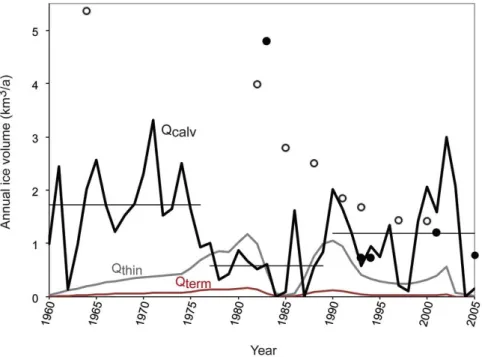
Fig. 12.Histories of surface thinningQthin(grey line) ice loss from the terminusQterm(dark red line), and calving fluxQcalv(black line) from 1960–2005. The calving fluxQcalvwas derived using the surface mass balance in input scenario #4 (Fig. 11). A piecewise linear fit was chosen to indicate averages during the periods 1960–1975, 1976–1990 and 1991–2005, as in Table 2 (thin black lines). The filled dots represent observed calving fluxes used to tune the models (listed in Table 1); the open dots represent calving fluxes modeled using a “sliding law”, listed in Table 3.
during 1976–1990, when Qbal was negative. There is cer-tainly the possibility that there have been years in which Qthin<0 when the climate was cooler and wetter, particu-larly during the period 1950–1970 and again around 1998– 2003, although there is no observational evidence to indicate thickening of the glacier during these periods.
Given the potential influence of calving speeds and retreat of the terminus on longitudinal extension in the terminal zone (e.g., Venteris et al., 1997), the rate of dynamic surface low-ering in the terminal zone must also have varied significantly during this period, but by how much is unknown, for only two direct measurements of the surface elevation of the lower reaches of the glacier exist, taken in 1975 and 2001 (Rivera et al., 2007). To first order, the rate of dynamic surface low-ering at any point on the glacier is a function of the change in glacier length and the local surface slope, i.e., longitudinal profile of the glacier surface; following this logic, thinning rates decrease upglacier from the terminus. Most glaciers with large volume losses exhibit a thinning pattern that in-creases with altitude (Schwitter and Raymond, 1993). Since we have little data to constrain the variability in dynamic thinning rates over this period, and noting that the parabolic longitudinal glacier surface profile is roughly maintained but shifts upvalley during retreat, we can calculate the rate of ice volume decrease represented by surface lowering and infer the temporal variability in the rate of thinning by combining the retreat history and trimlines on the valley walls and either
(1) assume that an average thinning rate of 2 m a−1was main-tained across the glacier surface throughout the period 1950– 2005 (to arrive at the average thinning rate of 0.35 km3a−1 stated above), or (2) assume that the dynamic thinning rate equals the product of the retreat rate and surface slope of the glacier in the lower reaches of the glacier, and then decreases upglacier to vanishing values at the glacier headwall. Calcu-lated in this latter way, and plotted in Fig. 12, the rate of ice volume lost to dynamic thinning increased to over 1 km3a−1 in the early 1980s and again in the late 1980s, when retreat accelerated markedly and calving rates increased. The com-bined thinning rate from dynamic surface lowering coupled with excess melt in the ablation zone most likely increased to almost 4 m a−1in the lower reaches of the glacier during this period.
5.4 Budgeting the calving flux
Table 3. Modeled velocities at the terminus using sliding, lateral drag and bathymetry developed in Benn et al. (2007) and Eqs. (8–12), for years with known terminus positions and bathymetric data, and observed terminus velocities for years with available data (Kondo and Yamada, 1988; Warren et al., 1995; Rignot et al., 1996; E. Rignot, personal communication, 2003). Calving speeds calculated according to definition in Eq. (8). Calving fluxesQcalvcalculated as product of calving speed and ice front areaAterm.
Year Modeled Observed Fjord Max Mean Retreat Calving Calving
terminus terminus halfwidth water water rate speed flux
velocity velocity W depth depth
(km a−1) (km a−1) (m) (m) (m) (m a−1) (km a−1) (km3a−1)
2001 3.40 3.08 1053 254 164 80 3.33 1.49
1998 3.25 1117 267 152 50 3.20 1.5
1994 3.32 4–6 1117 249 141 69 3.25 1.79
1992 3.51 1117 27 166 133 3.37 1.75
1989 4.72 1170 281 177 201 4.52 2.49
1986 5.01 1383 265 177 12 5.00 2.75
1983 6.17 5–8 1319 217 139 96 6.07 3.34
1976 7.91 1362 237 157 139 7.77 6.68
1965 6.01 1362 205 129 47 5.97 5.37
1959 8.95 1489 259 131 5 8.94 8.05
over the past 50 yr, the calving fluxQcalvalso takes into ac-count these ice mass losses (Qbal+Qthin+Qterm), as given in Eq. (7). Using this approach and our mass budget model with best fit scenario (case 4, where precipitation scales with k(z)and using the ablation co-efficients prescribed in Eq. 1a and 1b), the calving flux during the period 1960 to 2005 av-eraged 1.01 km3a−1(black line in Fig. 12), similar to fluxes calculated using InSAR in 2001.
As seen in Fig. 12 and Table 2,Qcalvas modeled using the mass budget has also varied significantly during the past half century. For example,Qcalvaveraged 1.8 km3a−1during the period 1960–1975, and decreased to less than 0.7 km3a−1 in the 1980s, a decade when surface melt rates increased and snow accumulation decreased so that all new accumu-lation was lost through abaccumu-lation and all calving resulted in net volume loss from the glacier. Qcalvslowly increased in the late 1990s to over 3 km3a−1, and decreased again in the first years of the 21st century. The corresponding calving ve-locities range from<1 km a−1to>7 km a−1over the 1960– 2005 period, in agreement with observations (Naruse, 1985; Kondo and Yamada, 1988; Rignot et al., 1996; Willis et al., 2010), and averaged 1.86 km a−1.
5.5 Calving fluxes modeled using the sliding law
The modeled annual velocities at the terminus using the sec-ond calving model, where the calving flux is driven by sliding at the terminus, withC=0.6 and constrained by the known terminus positions and water depths from Figs. 3 and 4, are listed in Table 3. The modeled velocities agree well with the observed surface velocities at the terminus from 1983, 1994, and 2001. Terminus velocities were very large between 1959–1979 (6–9 km a−1)when the glacier extended a
con-siderable distance into Laguna San Rafael and had substan-tially lower values of lateral drag. As the glacier receded to its present day position in the narrowing fjord, velocities de-creased to∼3.3 km a−1. Retreat rates are relatively insignif-icant (<200 m a−1)compared with the large velocities mod-eled at the terminus of the glacier, thus calving speeds were almost equal to down-glacier velocity (see Eq. 8). The re-sulting calving fluxes (the product of the calving velocityUD multiplied by the terminus cross-sectional areaAterm)follow a similar trend to the results from the mass budget model in Sect. 5.4, however, the magnitude of the calving fluxes range from∼6 km3a−1during 1960–1975, to 2.85 km3a−1 during 1976–1990, to 1.63 km3a−1as of 1990 (open dots in Fig. 12), exceeding those of the mass budget model (black line in Fig. 12) by between 40 % and 300 %.
The results from the “sliding law” model in Table 3 indi-cates a relatively robust correlation (r2=0.76) between the half width of the fjord channel and the modeled glacier ve-locity, suggesting that modeled ice velocities are driven pri-marily by changes in the channel width, where wide chan-nels allow for substantially lower values of lateral drag. In assuming plug flow in Eq. (12), it follows that the sliding ve-locity is most sensitive to changes in both ice thicknessHT relative to water depth and the glacier channel half-widthW. By comparison, the sliding model also indicates a negligible dependence on water depths: modeled calving velocities did not correlate with either mean water depth (r2=0.0008) or maximum water depth (r2=0.014).
Sensitivity analyses, carried out using the 2001 modeled calving velocity for its relatively good fit with observations (E. Rignot, personal communication, 2003; Willis et al., 2010), suggest that the calving velocity is particularly sus-ceptible to changes in tuning parameterC, in Eq. (11). Peak calving velocities occur whenC >3, where terminus veloci-ties approach 16 km a−1and any further increases inChave very little consequence. Similarly, whenCapproaches 0, the calving velocity also decreases rapidly, until it approaches zero. Raising the height above waterline (H0), adding to the vertical ice face at the terminus, also decreases ice ve-locity. Although an increase in ice thickness should en-hance the driving stress, it increases basal drag more substan-tially. While the driving stress is tempered by a low slope angle θ, the loading of ice onto the terminus will increase the downward pressure, increasing basal shear and lowering flow rates. Increasing the surface slope of the glacier, as-suming there are no other changes to the system, results in a power law increase in terminus velocity and hence calv-ing rate. Small increases in slope of the glacier would result in significant increases in the terminus velocity, allowing for rapid surges and appreciable increases in calving. This, how-ever, assumes that the same thickness of ice, and therefore the same downward acting forces will drive glacier flow. In re-ality, we would expect to see significant thinning associated with any increase in glacier slope, which has the potential to further enhance calving velocities.
The modeled calving fluxes using Benn et al.’s “sliding laws”, although greater than both observed and modeled mass balance fluxes, indicate a high degree of correlation between channel width, flow speed and calving rate. This behavior is key to understanding why most stable tidewa-ter glaciers have tidewa-termini located at topographic narrows, and why calving fluxes at Glaciar San Rafael decreased 2–5 fold, regardless of model scenario used, when the terminus re-treated into the narrowing outlet east of the Andean range front. However, the difference in the magnitude of the calv-ing fluxesQcalvbetween the sliding law model and mass bal-ance model also suggests that calving dynamics may be more variable than our simple approximation of plug flow and lat-eral drag, as used in Eqs. (10)–(12), would reflect.
5.6 Calving vs. retreat rates
Several studies have suggested that pronounced longitudinal stretching of glacier ice in the terminal zone may be a funda-mental feature of rapidly calving tidewater glaciers, promot-ing calvpromot-ing rates in excess of the balance flux of the glacier and resulting in retreat (e.g., Meier and Post, 1987; Venteris et al., 1997; Benn et al., 2007). If terminus retreat varies with increases in ice delivery to the terminus, as has been observed at other calving glaciers in the past decade (e.g., Howat et al., 2005; Luckman et al., 2006), retreat rates should increase in concert with increases in this calving flux. Our mass budget model results suggest the contrary, however; retreat rates ap-pear to have increased during periods when the calving flux decreased in the early 1980s and 1990s, while a short period of rapid retreat in the first few years of the 21st century ap-pears to coincide with an increase in the calving flux. This relationship holds whether the calving flux is modeled using an ice mass budget (Sect. 5.4) or using terminus velocities and ice front bathymetry (Sect. 5.5).
While we expect calving and terminus retreat to vary widely from glacier to glacier as each are dependent upon other factors, including the balance flux to the terminus and the rate of thinning (see Eq. 6), that the rate of retreat for San Rafael does not appear to co-vary with the calving flux in our models, and in fact, contrary to expectations appears pre-dominantly out of phase with Qcalv. These results appear robust, but do suggest that several of our inputs, assump-tions and sensitivities need revisiting. In particular, caution is needed with regard to (a) assuming that surface lower-ing occurs exclusively due to dynamic thinnlower-ing, (b) focus-ing the concentration of orographic precipitation around the ELA zone when using the surface mass balance to drive the model of ice fluxes, and (c) deriving basal sliding velocities and terminal ice fluxes from remotely sensed surface veloc-ities, which do not take into account longitudinal stretching and crevasse opening.
6 Implications for future behaviour
since the early 1980s. While a negative balance flux will con-tribute to increasing the retreat rate, accelerated thinning will retard it, so the two climatic drivers may be offsetting each other at San Rafael Glacier.
Contrary to what has been observed at other tidewater glaciers, such as the outlet glaciers of Greenland (Thomas et al., 2003; Howat et al., 2005; Stearns and Hamilton, 2007) or Marinelli Glacier in Tierra del Fuego (Koppes et al., 2009), negative balance flux and accelerated surface thinning at Glaciar San Rafael over the past few decades have not (as of yet) resulted in a substantial increase in the rate of terminus retreat. However, considering the ice thickness at the ELA is estimated to be only∼400 m (Rignot et al., 2003), con-tinuous thinning rates of 1–2 m a−1over the broad plateau of the icefield, where the ELA is located, would remove most of the glacier (and potentially most of the North Patagonian Ice-field) within a few hundred years. Such substantial changes in the balance flux and the ice thickness would also affect buoyancy at the glacier terminus. Furthermore, continuous rapid calving rates into water depths of∼210 m will likely destabilize the terminus and result in drastic retreat in the coming decades.
7 Conclusions
The annual budget of ice into and out of Glacier San Rafael over 1950–2005 was reconstructed using daily values of key climate variables from the NCEP-NCAR global reanalysis climate dataset and a compendium of historical observa-tions. Using a DEM of the glacier surface and this reanalysis dataset, constrained by a sparse collection of direct measure-ments of local temperature, precipitation, ablation and thin-ning collected over the past few decades and a documented retreat of the terminus over the past∼50 yr, we are able to es-timate the annual accumulation, ablation and thinning fluxes over the glacier and the corresponding calving flux from the terminus during this time.
San Rafael glacier experienced a period of accelerated re-treat starting around 1975 through the early 1990s, a period when accumulation decreased and ablation increased. Ter-minus retreat rates have been relatively low over the most re-cent decade, in part because the glacier is still experiencing rapid ice flow to the terminus and because it has retreated into a narrow outlet, limiting the contribution of ice-front melt to the overall mass loss. If our flux analysis is valid, the decrease in net accumulation and increase in ablation over the last few decades, as the climate has become warmer and drier, has primarily resulted in pervasive thinning through both surface mass loss and accelerated flow to the terminus, which has retarded terminus retreat. For Glaciar San Rafael, and possibly all glaciers of similar geometry with a broad plateau at the ELA and a narrow outlet, response to climate changes are reflected primarily in changes in the rate of sur-face thinning and the calving speed, and only secondarily in
changes in terminus position, emphasizing the complex dy-namics between climate inputs and glacier response.
Constrained by a few direct observations of Glaciar San Rafael’s dynamics over the past few decades, we have calcu-lated accumulation and ablation rates as a function of surface elevation to reconstruct the changing flux of ice to the ter-minus over the past ∼50 yr. Our mass budget approach is compared to a reconstructed calving flux using theoretical calving and sliding laws, and suggest that the trends in calv-ing fluxes are robust, with calvcalv-ing rates decreascalv-ing durcalv-ing periods of rapid retreat in the late 1970s and 1980s; how-ever, applying a “calving law” approach increases modeled calving rates by 40–300 %. Our approach provides a simple reconstruction of the time-varying budget of ice through San Rafael glacier using sparse empirical data which, when com-pared with the history of the terminus retreat gleaned from maps, aerial photos and satellite images, as well as with topo-graphic and bathymetric constraints of the lagoon into which it calves, illuminates the relative importance of climatic and non-climatic controls on glacier retreat on annual to decadal time scales.
Acknowledgements. This work was supported by US NSF grant OPP-0338371 (Koppes), and NASA subcontract #1267029 through Eric Rignot at JPL (Conway and Rasmussen). We thank Bernard Hallet for stimulating discussions and support of this work. We are most grateful to Gerard Roe for assistance with the orographic model, Andres Rivera for providing the Landsat imagery used in Fig. 1, Harvey Greenberg for assistance with the DEM con-struction, and Drew Stolar for assistance with GIS and MATLAB processing of the datasets.
Edited by: G. H. Gudmundsson
References
Aniya, M.: Glacier inventory for the Northern Patagonia Icefield, Chile, and variations 1944/45 to 1985/86, Arctic Alpine Res., 20, 179–187, 1988.
Aniya, M.: Recent glacier variations of the Hielos Patagonicos, South America, and their contribution to sea-level change, Arct. Antarct. Alp. Res., 31, 144–152, 1999.
Araneda, A., Torrej´on, F., Aguayo, M., Torres, L., Cruces, F., Cis-ternas, M., and Urrutia, R.: Historical records of San Rafael Glacier advances (North Patagonian Icefield): another clue to “Little Ice Age” timing in southern Chile?, Holocene, 17, 987– 998, 2007.
Benn, D. I., Hulton, N. R. J., and Mottram, R. H.: Calving laws, “sliding laws” and the stability of tidewater glaciers, Ann. Glaciol., 46, 123–130, 2007.
Cook, K. H., Yang, X., Carter, C. M., and Belcher, B. N.: A mod-eling system for studying climate controls on mountain glaciers with application to the Patagonian Icefields, Climate Change, 56, 339–367, 2003.
Dyurgerov, M. B. and Meier, M. F.: Mass balance of mountain and subpolar glaciers: a new global assessment for 1961–1990, Arc-tic Alpine Res., 29, 379–391, 1997.
Enomoto, H. and Nakajima, C.: Recent climate-fluctuations in Patagonia, in: Glaciological Studies in Patagonia Northern Ice-field 1983–1984, edited by: Nakajima, C., Nagoya (Japan), 7–14, 1985.
Escobar, F., Vidal, F., Garin, R., and Naruse, R.: Water balance in the Patagonain Icefield, in: Glaciological Researches in Patago-nia, 1990, edited by: Naruse, R. and Aniya, M., Nagoya (Japan), 109–119, 1992.
Fujiyoshi, Y., Kondo, H., Inoue, J., and Yamada, T.: Characteris-tics of precipitation and vertical structure of air temperature in northern Patagonia, Bull. Glacier Res., 4, 15–24, 1987. Hock, R.: Temperature index melt modeling in mountain areas, J.
Hydrol., 282, 104–115, 2003.
Hofer, M., M¨olg, T., Marzeion, B., and Kaser, G.: Empirical-statistical downscaling of reanalysis data to high-resolution air temperature and specific humidity above a glacier surface (Cordillera Blanca, Peru), J. Geophys. Res., 115, D12120, doi:10.1029/2009JD012556, 2010.
Howat, I. M., Joughin, I., Tulaczyk, S., and Gogineni, S.: Rapid re-treat and acceleration of Helhiem Glacier, east Greenland, Geo-phy. Res. Lett., 32, L22502, doi:10.1029/2005GL024737, 2005. Hubbard, A. L.: Modelling climate, topography and paleoglacier fluctuations in the Chilean Andes, Earth Surf. Proc. Land., 22, 79–92, 1997.
Hulton, N., Sugden, D., Payne, A., and Clapperton, C.: Glacier modeling and the climate of Patagonia during the Last Glacial Maximum, Quaternary Res., 42, 1–19, 1994.
Kalnay, E., Kanamitsu, M., Kistler, R., Collins, W., Deaven, D., Gandin, L., Iredell, M., Saha, S., White, G., Woollen, J, Zhu, Y., Chelliah, M., Ebisuzaki, W., Higgins, W., Janowiak, J., Mo, K. C., Ropelewski, C., Wang, J., Leetmaa, A., Reynolds, R., Jenne, R., and Joseph, D.: The NCEP/NCAR 40-year reanalysis project, B. Am. Meteorol. Soc., 77, 437–471, 1996.
Kerr, A. and Sugden, D.: The sensitivity of the South Chilean snow-line to climatic change, Climatic Change, 28, 255–272, 1994. Kistler, R., Kalnay, E., Collins, W., Saha, S., White, G., Woollen,
J., Chelliah, M., Ebisuzaki, W., Kanamitsu, M., Kousky, V., van de Dool, H., Jenne, R., and Fiorino, M.: The NCEP-NCAR 40-year reanalysis: monthly means CD-ROM and documentation, B. Am. Meteorol. Soc., 82, 247–267, 2001.
Kobayashi, S. and Saito, T.: Meteorological observations on Soler Glacier, in: Glaciological Studies in Patagonia Northern Icefield 1983–1984, edited by: Nakajima, C., Nagoya (Japan), 32–36, 1985.
Kondo, H. and Yamada, T.: Some remarks on the mass balance of the terminal-lateral fluctuations of San Rafael Glacier, the North-ern Patagonia Icefield, Bull. Glacier Res., 6, 55–63, 1988. Koppes, M., Hallet, B., and Anderson, J.: Synchronous
accelera-tion of ice loss and glacier erosion, Marinelli Glacier, Tierra del Fuego, J. Glaciol., 55, 207–220, 2009.
Koppes, M., Sylwester, R., Rivera, A., and Hallet, B.: Sediment yields over an advance-retreat cycle of a calving glacier, Laguna
San Rafael, North Patagonian Icefield, Quaternary Res., 73, 84– 95, 2010.
Koppes, M. N.: Glacier erosion and response to climate, from Alaska to Patagonia, University of Washington, Ph.D. thesis, 228 pp., 2007.
Lamy, F. J., Kaiser, J., Ninnemann, U., Hebbeln, D., Arz, H. W., and Stoner, J.: Antarctic timing of surface water changes off Chile and Patagonian ice sheet response, Science, 304, 959– 1962, 2004.
Luckman, A., Murray, T., de Lange, R., and Hanna, E.: Rapid and synchronous ice-dynamic changes in East Greenland, Geophys. Res. Lett., 33, L03503, doi:10.1029/2005GL025428, 2006. Matsuoka, K. and Naruse, R.: Mass balance features derived from
a firn core at Hielo Patagonico Norte, South America, Arct. Antarct. Alp. Res., 31, 333–340, 1999.
Mayr, C., Wille, M., Haberzetti, T., Fey, M., Janssen, S., Lucke, H., Ohlendorf, C., Oliva, G., Schabitz, F., Schleser, G. H., and Zolitschka, B.: Holocene variability of the Southern Hemi-sphere westerlies in Argentinean Patagonia (52◦S), Quaternary Sci. Rev., 26, 579–584, 2007.
Meier, M. F. and Post, A.: Fast tidewater glaciers, J. Geophys. Res., 92, 9051–9058, 1987.
Motyka, R. J., Hunter, L., Echelmeyer, K. A., and Connor, C.: Sub-marine melting at the terminus of a temperate tidewater glacier, LeConte Glacier, Alaska, U.S.A., Ann. Glaciol., 36, 57–65, 2003.
Naruse, R.: Flow of Soler Glacier and San Rafael Glacier, in: Glaciological Studies in Patagonia Northern Icefield 1983–1984, edited by: Nakajima, C., Nagoya (Japan), 32–36, 1985. Nye, J. F.: The flow of a glacier in a channel of rectangular elliptic
and parabolic cross-section, J. Glaciol., 5, 661–690, 1965. Ohata, T., Enomoto, H., and Kondo, H.: Characteristic of
abla-tion at San Rafael Glacier, in: Glaciological Studies in Patagonia Northern Icefield 1983–1984, edited by: Nakajima, C., Nagoya (Japan), 37–45, 1985a.
Ohata, T., Kondo, H., and Enomoto, H.: Meteorological observa-tions at San Rafael Glacier, in: Glaciological Studies in Patag-onia Northern Icefield 1983–1984, edited by: Nakajima, C., Nagoya (Japan), 22–31, 1985b.
O’Neel, S., Pfeffer, W. T., Krimmel, R., and Meier, M.: Evolving force balance and Columbia Glacier, Alaska, during rapid retreat, J. Geophys. Res., 110, F03012, doi:10.1029/2005JF000292, 2005.
Pfeffer, W. T.: A simple mechanism for irreversible tide-water glacier retreat, J. Geophys. Res., 112, F03S25, doi:10.1029/2006JF000590, 2007.
Powell, R. D.: Grounding-line systems as second-order controls on fluctuations of tidewater termini of temperate glaciers, in: Glacial marine sedimentation; Paleoclimatic significance, Geo-logical Society of America Special Paper 261, edited by: Ander-son, J. B. and Ashley, G. M., 75–94, 1991.
Rasmussen, L. A. and Conway, H.: Estimating South Cascade Glacier (Washington, U.S.A.) mass balance from a distance ra-diosonde and comparison with Blue Glacier, J. Glaciol., 47, 579– 588, 2001.
Rasmussen, L. A., Conway, H., and Raymond, C. F.: Influence of upper-air conditions on the Patagonia icefields, Global Planet. Change, 59, 203–216, 2007.
observations of Glaciar San Rafael, Chile, J. Glaciol., 42, 279– 291, 1996.
Rignot, E., Rivera, A., and Casassa, G.: Contribution of the Patag-onia Icefields of South America to sea level rise, Science, 302, 434–437, 2003.
Rignot, E., Koppes, M., and Velicogna, I.: Rapid submarine melting of the calving faces of west Greenland glaciers, Nat. Geosci., 3, 187–191, 2010.
Rivera, A., Benham, T., Casassa, G., Bamber, J., and Dowdeswell, J.: Ice elevation and areal changes of glaciers from the North Patagonia Icefield, Chile, Global Planet. Change, 59, 126–137, doi:10.1016/j.gloplacha.2006.11.037, 2007.
Roe, G. H.: Orographic precipitation, Ann. Rev. Earth Pl. Sc., 33, 645–671, 2005.
Schwitter, M. P. and Raymond, C. F.: Changes in the longitudinal profiles of glaciers during advance and retreat, J. Glaciol., 39, 582–590, 1993.
Smith, R. B. and Barstad, I.: A linear theory of orographic precipi-tation, J. Atmos. Sci., 61, 1377–1391, 2004.
Stearns, L. A. and Hamilton, G. S.: Rapid volume loss from two East Greenland outlet glaciers quantified using repeat stereo satellite imagery, Geophys. Res. Lett., 34, L05503, doi:10.1029/2006GL028982, 2007.
Thomas, R. H., Abdalati, W., Frederick, E., Krabill, W. B., Man-izade, S., and Steffen, K.: Investigation of surface melting and dynamic thinning on Jakobshavn Isbrae, Greenland, J. Glaciol., 49, 231–239, 2003.
Van der Veen, C.: Tidewater calving, J. Glaciol., 42, 375–385, 1996.
Venteris, E. R.: Rapid tidewater glacier retreat: a compari-son between Columbia Glacier, Alaska and Patagonian calving glaciers, Global Planet. Change, 22, 131–138, 1999.
Venteris, E. R., Whillans, I. M., and Van der Veen, C. J.: Effect of extension rate on terminus positions, Columbia Glacier, Alaska, USA, Ann. Glaciol., 24, 49–53, 1997.
Warren, C. R.: Rapid recent fluctuations of the calving San Rafael Glacier, Chilean Patagonia: climatic or non-climatic?, Geogr. Ann. A, 75, 111–125, 1993.
Warren, C. R. and Aniya, M.: The calving glaciers of southern South America, Global Planet. Change, 22, 59–77, 1999. Warren, C. R. and Sugden, D. E.: The Patagonian Icefields: a
glaciological review, Arctic Alpine Res., 25, 316–331, 1993. Warren, C. R., Glasser, N. F., Harrison, S., Winchester, V., Kerr, A.,
and Rivera, A.: Characteristics of tide-water calving at Glaciar San Rafael, Chile, J. Glaciol., 41, 273–289, 1995.
Willis, M. J., Melkonian, A. K., Pritchard, M. E., and Bernstein, S.: Remote sensing of velocities and elevation changes at outlet glaciers of the Northern Patagonian Icefield, Chile, International Glaciological Conference Ice and Climate Change: A View from the South. Valdavia, Chile, February 2010.
Wratt, D. S., Revell, M. J., Sinclair, M. R., Gray, W. R., Henderson, R. D., and Chater, A. M.: Relation between mass properties and mesoscale rainfall in New Zealand’s Southern Alps, Atmos. Res., 52, 261–282, 2000.