A flexible three-dimensional stratocumulus, cumulus and cirrus cloud generator (3DCLOUD) based on drastically simplified atmospheric equations and Fourier transform framework

(1)

GMDD

7, 295–337, 2014

A flexible 3-D stratocumulus, cumulus and cirrus

cloud generator

F. Szczap et al.

Title Page

Abstract Introduction

Conclusions References

Tables Figures

◭ ◮

Back Close

Full Screen / Esc

Printer-friendly Version Interactive Discussion

Discussion

P

a

per

|

D

iscussion

P

a

per

|

Discussion

P

a

per

|

Discuss

ion

P

a

per

|

Geosci. Model Dev. Discuss., 7, 295–337, 2014 www.geosci-model-dev-discuss.net/7/295/2014/ doi:10.5194/gmdd-7-295-2014

Open Access

Geoscientiic

Model Development Discussions

This discussion paper is/has been under review for the journal Geoscientific Model Development (GMD). Please refer to the corresponding final paper in GMD if available.

A flexible three-dimensional

stratocumulus, cumulus and cirrus cloud

generator (3DCLOUD) based on

drastically simplified atmospheric

equations and Fourier transform

framework

F. Szczap1, Y. Gour1, T. Fauchez2, C. Cornet2, T. Faure3, O. Jourdan1, and P. Dubuisson2

1

Laboratoire de Météorologie Physique, UMR6016, CNRS, Aubière, France

2

Laboratoire d’Optique Atmosphérique, UMR8518, CNRS, Villeneuve d’Ascq, France

3

Laboratoire d’Ingénierie pour les Systèmes Complexes, Clermont-Ferrand, France

Received: 31 October 2013 – Accepted: 21 December 2013 – Published: 14 January 2014

Correspondence to: F. Szczap ([email protected])

(2)

GMDD

7, 295–337, 2014

cloud generator

F. Szczap et al.

Title Page

Tables Figures

◭ ◮

Back Close

Full Screen / Esc

Discussion

P

a

per

|

D

iscussion

P

a

per

|

Discussion

P

a

per

|

Discuss

ion

P

a

per

|

Abstract

The 3DCLOUD algorithm for generating stochastic three-dimensional (3-D) cloud fields is described in this paper. The generated outputs are 3-D optical depth (τ) for stratocu-mulus and custratocu-mulus fields and 3-D ice water content (IWC) for cirrus clouds. This model is designed to generate cloud fields that share some statistical properties observed in

5

real clouds such as the inhomogeneity parameterρ(standard deviation normalized by the mean of the studied quantity), the Fourier spectral slopeβclose to₋5/3 between the smallest scale of the simulation to the outerLout(where the spectrum becomes flat). Firstly, 3DCLOUD assimilates meteorological profiles (humidity, pressure, temperature and wind velocity). The cloud coverageC, defined by the user, can also be assimilated,

10

but only for stratocumulus and cumulus regime. 3DCLOUD solves drastically simplified basic atmospheric equations, in order to simulate 3-D cloud structures of liquid or ice water content. Secondly, Fourier filtering method is used to constrain intensity of ρ, β, Lout and mean of τ or IWC of these 3-D cloud structures. 3DCLOUD model was developed to run on a personnel computer under Matlab environment with the Matlab

15

statistics toolbox. It is used to study 3-D interactions between cloudy atmosphere and radiation.

1 Introduction

Clouds have a significant effect on the Earth radiation budget. They reflect the so-lar radiation and reduce the warming of the Earth (albedo effect). They also create

20

a greenhouse effect by trapping the thermal radiation emitted from the Earth surface, reducing the radiative cooling of the Earth (Collins and Satoh, 2009). Cloud feedback remains however the largest uncertainty in the study of climate sensitivity for almost twenty years (Bony et al., 2006). In almost all climate models, clouds are assumed plane-parallel with homogeneous optical properties (PPH) and radiation codes use

25

one-dimensional (1-D) scheme. Therefore, improving parameterisations of clouds in

(3)

GMDD

7, 295–337, 2014

cloud generator

F. Szczap et al.

Title Page

Tables Figures

◭ ◮

Back Close

Full Screen / Esc

Discussion

P

a

per

|

D

iscussion

P

a

per

|

Discussion

P

a

per

|

Discuss

ion

P

a

per

|

large-scale model, especially their interaction with radiation, is a challenge in order to reduce uncertainty in model projections of the future climate (Illingworth and Bony, 2009). Improved global characterization of the three dimensional (3-D) spatial distribu-tion of clouds is thus necessary (Clothiaux et al., 2004).

Moreover, satellite passive and active sensors such as spectral and

multi-5

angular radiometers, LIDAR, RADAR in the A-train mission allow the retrieval of cloud horizontal and vertical optical properties with an adequate spatial and temporal cov-erage. For practical and computational cost purposes, interpretation of such measure-ments generally also assumes 1-D radiative algorithm and PPH cloud. This assump-tion can be far from being realistic and leads to biases on the retrieved properties from

10

passive sensors (Barker and Liu, 1995; Várnai and Marshak, 2002, 2007; Lafont and Guillemet, 2004; Cornet et al., 2005, 2013) and active sensors (Battaglia and Tanelli, 2011). These biases are at least, function of the cloud coverage and of the variability of cloud optical depth or water content. This variability is quantified by an inhomogeneity parameter, often defined as the standard deviation normalized by the mean of the

stud-15

ied quantity (Szczap et al., 2000; Carlin et al., 2002; Oreopoulos and Cahalan, 2005; Sassen et al., 2007; Hill et al., 2012).

Determining the significance of the 3-D inhomogeneity of clouds for climate and re-mote sensing applications requires to measure and to simulate the full range of actual cloud structure. Set apart the computational time, accurate 3-D cloudy radiative

trans-20

fer problem is not an issue, per se (Evans and Wiscombe, 2004). Monte Carlo transfer models can indeed accurately and efficiently compute radiative properties for arbitrary cloud fields (Battaglia and Mantovani, 2005; Pincus and Evans, 2009; Mayer, 2009; Cornet et al., 2010; Battaglia and Tanelli, 2011). The difficulty is to generate cloud property fields that are statistically representative of cloud field in nature. Cloud fields

25

(4)

GMDD

7, 295–337, 2014

cloud generator

F. Szczap et al.

Title Page

Tables Figures

◭ ◮

Back Close

Full Screen / Esc

Discussion

P

a

per

|

D

iscussion

P

a

per

|

Discussion

P

a

per

|

Discuss

ion

P

a

per

|

models have the capacity to simulate quickly realistic 2-D and 3-D cloud structures with just a few parameters. Examples of these types of cloud models are: the bounded cas-cade model (Cahalan et al., 1994; Marshak et al., 1998), the IAAFT algorithm (Venema et al., 2006), the SITCOM model (Di Guiseppe and Thompkins, 2003), the tdMAP model (Benassi et al., 2004), the model developed by Evans and Wiscombe (2004) for

5

low liquid clouds (stratocumulus and cumulus) or by Alexandrov et al. (2010) and the Cloudgen model (Hogan and Kew, 2005) for high ice clouds (cirrus). These stochas-tic models are based on fractal or Fourier framework. The scale invariant properties observed in real clouds can be controlled. The power spectra of the logarithm of their optical properties (optical depth, liquid water content or liquid water path for low clouds

10

and ice water content for high clouds) typically exhibits a spectral slope of around₋5/3 (Davis et al., 1994, 1996, 1997, 1999; Cahalan et al., 1994; Benassi et al., 2004; Hogan and Kew, 2005; Hill et al., 2012; Fauchez et al., 2013) from small scale (a few meters) to the “integral scale” or the outer scale (few ten to hundred kilometers), where the spectrum becomes flat (decorrelation occurs). The disadvantage of such model lies in

15

that effects of meteorological processes are poorly considered and dominant scales of organization related to turbulent eddy due, for example, to wind shear, convection, entrainment are not considered.

The aim of the 3DCLOUD algorithm is to reconcile these two approaches. In Sect. 2, we describe the 3DCLOUD generator. In Sect. 3, 3DCLOUD outputs are compared to

20

LES outputs to check the validity of the chosen basic atmospheric equations. In Sect. 4, stratocumulus, cumulus and cirrus examples provided by 3DCLOUD are presented.

2 The 3DCLOUD generator

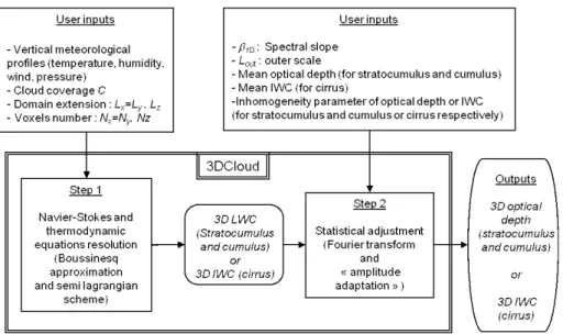
3DCLOUD generates, in two distinct steps (see Fig. 1), a 3-D optical depth field for stratocumulus and cumulus or a 3-D ice water content field for cirrus clouds. These

25

cloud fields were chosen as most of the papers dealing with scale invariant proper-ties focus on liquid water path and optical depth for stratocumulus and cumulus and

(5)

GMDD

7, 295–337, 2014

cloud generator

F. Szczap et al.

Title Page

Tables Figures

◭ ◮

Back Close

Full Screen / Esc

Discussion

P

a

per

|

D

iscussion

P

a

per

|

Discussion

P

a

per

|

Discuss

ion

P

a

per

|

on ice water content for cirrus. During the first step, meteorological vertical profiles (temperature, pressure, wind, humidity), defined by the user, are assimilated and ba-sic atmospheric equations are resolved. During the second step, cloud scale invariant properties are constrained in a Fourier framework. At the same time, a gamma distri-bution of local optical depth or IWC is mapped onto the LWC/IWC generated during the

5

first step. This gamma distribution is iteratively computed in such way that the mean optical depth or IWC and the inhomogeneity parameter satisfy the values imposed by the user. Details of these two steps are now presented.

2.1 Step 1: the 3-D LWC/IWC generator

The essential basic quantities to generate cloud fields are the condensed water mixing

10

ratioqc=ql+qiwhereqlis the liquid water mixing ratio andqi is the ice water mixing ratio, the wind velocity vectoru, air pressurep, temperatureT, and vapour water mixing ratioqv. Mixing ratios are the mass of vapour or condensed water per unit of dry air mass. We describe in this section, the equations used to generate clouds with the associated simplifications used.

15

2.1.1 The simplification of basic atmospheric equations

The movement of air parcels in the atmosphere is governed by second law of Newton and can be written (Houze, 1993):

du

dt =− 1

ρ∇p−fk∧u−gk+F (1)

wheretis time,ρthe air density,f the Coriolis parameter,gis the acceleration due to

20

gravity andF the acceleration due to other forces (frictional acceleration for example). d/dt=∂/∂t+u_{· ∇}is the Lagrangian derivative operator following a parcel of air,∂/∂t is the Eulerian derivative operator and ∇is the three-dimensional gradient operator.

(6)

GMDD

7, 295–337, 2014

cloud generator

F. Szczap et al.

Title Page

Tables Figures

◭ ◮

Back Close

Full Screen / Esc

Discussion

P

a

per

|

D

iscussion

P

a

per

|

Discussion

P

a

per

|

Discuss

ion

P

a

per

|

componentw projected into the Cartesian geometry system, wherei,jandk are the unit vectors in thex,y andz directions.

When the phase changes are only associated with condensation and evaporation of water, the first law of thermodynamics can be written (Houze, 1993):

dθ dt =−

L cp

Qdq_dtv (2)

5

whereL=2500 kJ kg−1 andL=2800 kJ kg−1 are the usual latent heat of vaporization of water and ice, respectively.cp=1.004 kJ kg−

1

K−1 is the usual specific heat of dry air at constant pressure,θ is the potential temperature andQ=(p/p0)

κ

=T/θ is the Exner function wherep0=1000 hPa andκ=0.286.

In addition to the equation of motion and the first law of thermodynamics, parcels of

10

air obey the continuity equation

dρ

dt =−ρ∇ ·u (3)

and the water continuity equation

dqi

dt =Si, i =1,. . .,n (4)

where Si are the sum of the sources and sinks for a particular category (among n

15

categories) of water indicated byi (vapor, solid, liquid water category for example). The horizontal extension of the simulated stratiform cloud fields is around 10 km. We can thus assume a constant horizontal pressure. Moreover, for stratocumulus, cu-mulus and cirrus clouds fields, the vertical extension of air motions remains confined to a shallow layer, we can apply the Boussinesq approximation, which implies that

20

the atmosphere is an incompressible fluid and the buoyancy forces are function of the virtual potential temperature. At last, we assume an atmosphere characterized by

(7)

GMDD

7, 295–337, 2014

cloud generator

F. Szczap et al.

Title Page

Tables Figures

◭ ◮

Back Close

Full Screen / Esc

Discussion

P

a

per

|

D

iscussion

P

a

per

|

Discussion

P

a

per

|

Discuss

ion

P

a

per

|

a high Reynolds number as inviscid fluid and we assume that the Coriolis parameter is negligible. These considerations lead to a dramatically simplification of the dynamic equations. The simplified equations of 3DCLOUD governing the formation of 3-D cloud structures are:

                

du

dt =g( θ∗v

θ_v0 −qc)k

∇ ·u₌0 dθ

dt = L c_pQξ

dq_v

dt =−ξ

dqc

dt =ξ

(5)

5

where we denote the reference state by subscript0 and deviation from the reference state by an asterisk, θv=θ(1+0.61qv) is the virtual potential temperature. For stra-tocumulus and cumulus fieldsξ is estimated as:

ξ=min(qvs−qv,qc)∆t (6)

where∆tis the simulation time step, the saturation mixing ratioqvs(T,p) is derived from

10

Thetens and Magnus formula and is given byqvs(T,p)=

0.622P_sat

(p/100₋0.378Psat), where for

wa-ter,P_sat=6.107 exp[_234.82(4028(T−_T273.15)

−38.33)], and for ice,Psat=6.107×10

[ 9.5(T−273.15)

265.5+(T−273.15)]_{. Because}

the saturation mixing ratio qvs is a function of temperature, computation of ξ at each simulation step is based on the work of Asai (1965). For cirrus clouds, condensation, evaporation and ice crystals sedimentation processes are very complex and still not

15

(8)

GMDD

7, 295–337, 2014

cloud generator

F. Szczap et al.

Title Page Abstract Introduction Conclusions References Tables Figures ◭ ◮ ◭ ◮ Back Close

Full Screen / Esc

Printer-friendly Version Interactive Discussion Discussion P a per | D iscussion P a per | Discussion P a per | Discuss ion P a per |

vfall taken from Starr and Cox (1985):

vfall= 1.5

6 log 10[max(IWC, 1×10

−6_)]

+1.5 (7)

wherevfall is in m s− 1

and the ice water content IWC in g m−3.

2.1.2 Assimilation of meteorological profiles and cloud coverage

In order to control the structure and nature of clouds and especially vertical position

5

and extension, it is necessary to impose a large-scale environment. Practically, forcing terms are added into the 3DCLOUD equations to nudge the solutions towards obser-vations. Our state observations are the initial meteorological profiles (provided by the user for example) and do not change during the simulation. The technique used is based on the initialization integration method (Pielke, 2002). Consequently, 3DCLOUD

10 equations become:                            du

dt =Gu(z) [uini(z)−u(z)]¯ dv

dt =Gv(z) [vini(z)−v¯(z)] dw

dt =g _θ∗

v

θ_v₀−qc

∇ ·u₌0 dθ

dt = L

c_pQξ+Gθ(z)[θini(z)−θ] dq_v

dt =−ξ+Gq_v(z)[qv_ini(z)−qv] dqc

dt =ξ

(8)

where for variables X, ¯X(z) is the mean of X at height z and quantities GX(z) are

adjusted during the simulation in such a way thatX or ¯X(z) do not diverge far away from initial conditions Xini(z). In a general way, G is the inverse of timescale but

be-15

(9)

GMDD

7, 295–337, 2014

cloud generator

F. Szczap et al.

Title Page

Tables Figures

◭ ◮

Back Close

Full Screen / Esc

Discussion

P

a

per

|

D

iscussion

P

a

per

|

Discussion

P

a

per

|

Discuss

ion

P

a

per

|

equations and should be scaled by the slowest physical adjustment processes in the model (Cheng et al., 2001). We first set this timescale to 1 h. Nevertheless, we no-ticed empirically that 1 h timescale is too large and must be modified as a function of height, especially at height where the vertical gradient ofX is large (at the top of a stratocumulus cloud for example). Therefore, we developed a very fast and simple

5

numerical method to adjust the values of GX(z) during the simulation. At each level,

we compute the relative differenceα_X(z)=Xini(z)−X(z)

X(z) ·100.GX(z) is assumed to be pro-portional toαX(z) and is estimated asGX(z)=min[Gmin+

G_max−G_min

αX,max αX(z),Gmax] where

Gmin=36001 s

−1

and Gmax=21∆t. The values of αX,max were estimated during our nu-merous numerical experiments. For stratocumulus and cumulus,α_X,maxvalues for

hor-10

izontal wind, temperature and humidity are 20 %, 2 % and 20 % respectively and for cirrus,αX,maxvalues are 20 %, 10 % and 10 %, respectively.

The cloud coverageCis defined as the fraction of the number of cloudy pixels to the total number of pixel in the 3DCLOUD field projected onto the 2-D horizontal plan. The value ofCis chosen with the assimilation of initial meteorological profiles. At each time

15

step, the initial profile of vapour mixing ratio qv_ini(z) is modified between cloud base and top height ifC_≥50 % or between ground and cloud top height if C <50 % untilC agrees with the desired value within few per cents. The new “initial” profile of vapour mixing ratioqvnew_ini (z) is computed from currently simulated (old) profile of vapour mixing ratioqvold_ini(z) asq

new v_ini (z)=q

old v_ini(z)±

nz−nbase

n_top₋n_baseq

old

v_ini(z)×1000.1 wherez is height,nz,ntopand

20

nbase are the index of level inzdirection for cloud top height and for cloud base height (or ground), respectively.

(10)

GMDD

7, 295–337, 2014

cloud generator

F. Szczap et al.

Title Page

Tables Figures

◭ ◮

Back Close

Full Screen / Esc

Discussion

P

a

per

|

D

iscussion

P

a

per

|

Discussion

P

a

per

|

Discuss

ion

P

a

per

|

2.1.3 Implementation of 3DCLOUD algorithm

To implement the previously described equations, space is divided into (N_x+2)×

(N_y+2)_×(N_z+2) cells or voxels whereN_x,N_y andN_z are the voxel numbers in each direction. A voxel is characterized by its spatial resolution with_∆x= ∆y6= ∆z. Horizon-tal extensions areL_x=L_y and can be different of the vertical extensionL_z. In order to

5

take account of boundary conditions, one layer of voxel is added around the simulation domain.

We adopted a semi-Lagrangian scheme to solve the equation: dX

dt = ∂X

∂t +u· ∇X=0 (9)

whereX is a scalar advected by the wind velocityu.X can be the potential

temper-10

ature θ, the condensed water qc or the vapor mixing ratios qv, and also the three components of wind velocity u, v and w. Two steps are needed in order to compute the value of X(x,t+ ∆t) at a fixed position x and at time t+ ∆t. X(x,t) and u(x,t) are known values and ∆t is the time step. Firstly, we compute the previous position p(X,t₋∆t)=x₋u(x,t)∆tofX at timet₋∆t. Secondly, we compute the value ofX(p,t)

15

at the positionpand at the time t by an interpolation scheme. This interpolated value X(p,t) is the desired valueX(x,t+ ∆t). The major advantage of this approach is that the time step is not restricted by the Courant–Friedrichs–Lewy stability limit but by the less restrictive condition that parcels do not overtake each other during the time step (Riddaway, 2001). Therefore, at each iteration, the maximum value of time step∆tmax

20

can be roughly estimated as∆tmax=_max 1

|∆u

∆x|+max|∆ v

∆y|+max|∆ w

∆z|

. The accuracy of this

ap-proach depends on the accuracy of the interpolation scheme. Due to CPU time, we chose a linear interpolation, which unfortunately provides numerical dissipations. How-ever, this drawback is overcome using the Fourier transform performed in the second step of the 3DCLOUD algorithm (see Sect. 2.2.2).

25

Fourier transform is very easy to implement, we chose thus this method to solve the equation_{∇ ·}u₌0. In the Fourier domain, the gradient operator _∇is equivalent to the

(11)

GMDD

7, 295–337, 2014

cloud generator

F. Szczap et al.

Title Page

Tables Figures

◭ ◮

Back Close

Full Screen / Esc

Discussion

P

a

per

|

D

iscussion

P

a

per

|

Discussion

P

a

per

|

Discuss

ion

P

a

per

|

multiplication byik, where i_≡√₋1 and k is the wave number vector. The following equationik_·uˆ(k)=0 has thus to be solved, whereuˆ is the transform of wind velocity

uin the Fourier domain. This implies that the Fourier transform of velocity of a diver-gent free field is always perpendicular to its wave numbers. Therefore, the quantity 1/k2(k_·uˆ(k))k is removed from uˆ. Keeping the real part of inverse transform of uˆ

5

provides the new wind velocityuwith the desired divergent free property.

Lateral periodic conditions and continuity conditions to bottom and top are applied. For wind velocity, free slip boundary condition is applied at the bottom and top of the domain, which are assumed to be a solid wall (i.e.w=0). But as the Fourier transform (which is needed to solve the equation_∇·u₌0) requires periodic conditions, it provides

10

spurious oscillations during the simulations. In order to limit this effect, extra levels with wind velocity set to zero are added under and above the model domain.

The algorithm of 3DCLOUD in order to simulate 3-D structures of LWC or IWC is, in summary:

1. Definition of initial meteorological profilesuini, vini, θini,qv_ini from idealized cloud

15

conceptual models or from the user. Vertical pressure profile is generally com-puted from the hydrostatic law but can be provided by the user.

2. Initial perturbationsu′ are added to wind velocityu.u′ is free-divergent and tur-bulent with a spectral slope of−5/3 (see more explanations in Sect. 2.2.2).

3. Assimilation of initial meteorological profiles (optional, see Eq. 8 and Sect. 2.1.2).

20

4. Constrain of divergent-free velocityu(see Eq. 8).

5. Computation of ice fall speedvfall(only for cirrus cloud, see Eq. 7).

6. Advection ofu,v,w,θ,qvandqcby wind velocityu(see Eq. 9).

7. Modification of θ, qv and qc due to evaporation/condensation processes (see Eq. 6).

(12)

GMDD

7, 295–337, 2014

cloud generator

F. Szczap et al.

Title Page

Tables Figures

◭ ◮

Back Close

Full Screen / Esc

Discussion

P

a

per

|

D

iscussion

P

a

per

|

Discussion

P

a

per

|

Discuss

ion

P

a

per

|

8. Modification of the vertical velocity due to buoyancy (see Eq. 8)

9. Modification of q_v

ini in order to assimilate cloud coverage C (optional, only for

stratocumulus and cumulus, see Sect. 2.1.2).

10. Return to Eq. (3) until maximum iteration number is reached.

11. Computation of LWC or IWC, where LWC or IWC₌ρairqc and ρair is density of

5

air.

2.2 Step 2: statistical adjustment

We present hereafter the step 2 of 3DCLOUD, the methodology able to adjust, ac-cording to user requirements, the mean optical depth ¯τ(or the mean ice water content IWC) and the inhomogeneity parameter of the optical depthρτ (or the ice water

con-10

tentρIWC) from the LWC (or from the IWC) simulated at the step 1. The distribution of τor IWC is assumed to follow a gamma distribution. Indeed, distribution ofτand IWC could usually be well represented by a lognormal or gamma distribution (Cahalan et al., 1994; Barker et al., 1996; Carlin et al., 2002; Hogan and Illingworth, 2003; Hogan and Kew, 2005). The scale invariant cloud properties are controlled at each level. They are

15

characterised by the spectral exponentβ1-D close to−5/3 (slopeβof the one dimen-sion wave number spectrum in log–log axes of Fourier space) of the local optical depth or the IWC. This spectral slope is computed from the outer scaleL_out (defined by the user) to the smaller scale (voxel horizontal size).

2.2.1 Control of the mean and of the inhomogeneity parameter

20

The relation betweenlocal optical depthτ(x,y,z), liquid water path LWP and density of waterρlin each voxel is given by (Liou, 2002):

τ(x,y,z)= 3

2ρl

LWP(x,y,z) Reff

with LWP(x,y,z)=ρairqc(x,y,z)∆z (10)

(13)

GMDD

7, 295–337, 2014

cloud generator

F. Szczap et al.

Title Page

Tables Figures

◭ ◮

Back Close

Full Screen / Esc

Discussion

P

a

per

|

D

iscussion

P

a

per

|

Discussion

P

a

per

|

Discuss

ion

P

a

per

|

where x, y, z are spatial positions inside the simulation domain, LWP(x,y,z) is the

localliquid water path and_∆z is the vertical resolution.Local quantity means that the

quantity is estimated inside a voxel. The optical depthτ(x,y) for each pixel is the sum

oflocaloptical depths along thezaxis:

τ(x,y)= Nz

X

z=1

(x,y,z). (11)

5

The mean optical depth ¯τis then defined as:

¯

τ= 1

N_xN_y

Nx

X

x=1

Ny

X

y=1

τ(x,y). (12)

In the same way, for ice cloud, the mean IWC is obtained with

IWC= 1

N_xN_yN_z∗

N_x X

x=1

Ny

X

y=1

N_z∗ X

z=1

IWC(x,y,z) (13)

whereNz∗ is the number of layer between the cloud top layer and cloud bottom layer.

10

To describe the amplitude of the optical depth for 1-D and 2-D overcast cloud, Szczap et al. (2000) defined the inhomogeneity parameter of optical depthρ_τ. For 3-D broken fields, this parameter is defined according to

ρτ=

σ[τ>0(x,y)] ¯

τ>0_(x,y₎ (14)

where σ[τ>0(x,y)] and ¯τ>0(x,y) are the standard deviation and the mean of strictly

15

(14)

GMDD

7, 295–337, 2014

cloud generator

F. Szczap et al.

Title Page

Tables Figures

◭ ◮

Back Close

Full Screen / Esc

Discussion

P

a

per

|

D

iscussion

P

a

per

|

Discussion

P

a

per

|

Discuss

ion

P

a

per

|

Due to the flexibility of the mathematical formulation of the gamma distribution and to its ability to mimic the attributes of other positive-value distributions such as log-normal and exponential distribution, we choose to control ¯τ or IWC and ρ_τ or ρIWC by mapping theoretical gamma-distributed properties onto the simulated properties. This mapping technique is analog to the “amplitude adaptation” technique explained

5

in Venema et al. (2006), where amplitudes are adjusted based on their ranking. The gamma distribution is a two-parameter family of continuous probability distribution. It has a shape parameteraand scale parameterb. The equation defining the probability density as a function of a gamma-distributed random variableY is:

Y =f(µ;a,b)= 1

ba_Γ_(a)µ

a−1_e−µ/b ₍₁₅₎

10

whereΓ(.) is the gamma function. We develop a simple iterative algorithm, where val-ues ofa andb are adjusted until mean and inhomogeneity parameters reach the re-quired user values within few percent.

2.2.2 Control of invariant scale properties by adjustment of spectral exponent in Fourier space

15

The spectral slope valueβ1-D of the horizontally 2-D field is adjusted according to the following methodology. As proposed by Hogan and Kew (2005), we choose to manip-ulate 2-D plan of Fourier amplitudes oflocal optical depthτ2-D (or IWC2-D) with a 2-D Fourier transform performed at each height of cloudy layer. Suppose a 2-D isotropic fieldg(x,y) characterized by a Gaussian probability density function (PDF) and a 1-D

20

power spectrumE1(k) with a spectral slopeβ1-D at all scales defined as:

E1(k)=cE1k−β1-D (16)

wherekis the wave number in any direction andcE1is the spectral energy density atk= 1 m−1. Following Hogan and Kew (2005), for idealized case whereg(x,y) is continuous

(15)

GMDD

7, 295–337, 2014

cloud generator

F. Szczap et al.

Title Page

Tables Figures

◭ ◮

Back Close

Full Screen / Esc

Discussion

P

a

per

|

D

iscussion

P

a

per

|

Discussion

P

a

per

|

Discuss

ion

P

a

per

|

at small scales and infinite in extend, its 2-D spectral density matrixE2(kx,ky) can be

written as

E2(k)=κcE1k−β1-D−1 (17)

wherek= q

k_x2+k_y2andκa constant. In general, a 2-D cloud layer ofτ2-D (or IWC2-D) is anisotropic and in our case the optical depth (or IWC) is gamma-distributed.

There-5

fore the 1-D power spectrumE₁(k) has seldom the required spectral slopeβ_1-D. In this context, a numerical method has to be developed to perform our objectives.

Let setYd2-D the 2-D Fourier transform ofY2-D, whereY2-D can beτ2-D (or IWC2-D) at a given cloudy layer. This quantity, estimated with the help of a direct 2-D Fast Fourier Transform algorithm can be written as

10

d

Y2-D(k)=E2-D(k) exp(i φ2-D(k)) (18)

whereE2-D=|Yd2-D|is the magnitude or spectral energy,φ2-D(k) are the phase angles

andk= q

k_x2+k_y2 is the absolute wave number. The cloud field domain is defined to measure L_x and L_y and they have spatial resolutions of ∆x and ∆y. The resulting wave number forE2-D ranges from−Kx to+Kxwith a resolution of∆kx=1/Lx, where

15

Kx=1/2∆x. It is similar forky direction.

Our objective is to modify spectral energyE2-D(k) in such a way that the 1-D spec-tral slope value µ1-D estimated in one dimension from Y2-D fork≥kout (kout=1/Lout) satisfies the desired valueβ1-Drequired by the user. Practically,µ1-D is defined as:

µ1-D=(βx+βy)/2 (19)

20

whereβx and βy are the 1-D spectral slope values of Yd2-D estimated in the x and y directions respectively.

(16)

GMDD

7, 295–337, 2014

cloud generator

F. Szczap et al.

Title Page

Tables Figures

◭ ◮

Back Close

Full Screen / Esc

Discussion

P

a

per

|

D

iscussion

P

a

per

|

Discussion

P

a

per

|

Discuss

ion

P

a

per

|

kout, two 2-D matrixE2-D∗ (k) andE2-D∗∗ (k) can be computed.E2-D∗ (k) is based on Eq. (22) and is defined as:

E_2-D∗ (k)=k

(₋β1-D−1)

k(−β1-D−1)

out

E2-D(k=kout) (20)

whereasE_2-D∗∗ (k) is defined as:

E_2-D∗∗ (k)=E2-D(k)

E2-D(k)

k(−β1-D−1)

out

E2-D(k=kout) (21)

5

whereX is the mean of variableX. If the degree of anisotropy ofY2-D is small, such as for stratocumulus and cumulus, we useE_2-D∗ (k) and if not, such as for cirrus clouds, E_2-D∗∗ (k). Nonetheless, the user can also choose one of these methods.

Finally, the new 2-Dlocaloptical depth (or the 2-D new ice water contentY_2-Dnew) at the given cloudy layer is computed by keeping the real part of the inverse 2-D Fast Fourier

10

Transform of the new quantity:

[

Y_2-Dnew(k)=E_2-D∗ (k) exp(i φ2-D(k)) orY[_2-Dnew(k)=E_2-D∗∗ (k) exp(i φ2-D(k)) (22)

But as a result, the distribution ofY_2-Dnew is not the sameY2-D at the given cloudy layer, and the equality between the estimated spectral slopeµ1-D of Y

new

2-D and the required valuesβ1-Dis not always guaranteed. Therefore, we have to redo an “amplitude

adap-15

tation”, as explained in Venema et al. (2006), and to iterate the process explained in this section by changing the value ofβ1-D in Eqs. (20) or (21), until the estimated value µ1-D reaches the required value within few percent.

(17)

GMDD

7, 295–337, 2014

cloud generator

F. Szczap et al.

Title Page

Tables Figures

◭ ◮

Back Close

Full Screen / Esc

Discussion

P

a

per

|

D

iscussion

P

a

per

|

Discussion

P

a

per

|

Discuss

ion

P

a

per

|

2.2.3 Implementation

We describe here the part of 3DCLOUD algorithm that establishes the cloud field mean optical depth ¯τ (IWC), the inhomogeneity parameterρ_τ (or ρIWC) and the spectral ex-ponentβ1-D.

For stratocumulus and cumulus clouds, algorithm is as follows:

5

1. Transformation of LWC(x,y,z) toτ_3-D′ (x,y,z) with Eq. (10). Effective radius can be set to 10 µm for example.

2. Application of the algorithm explained in Sect. 2.2.2 in order to constrainβ1-D of each cloudy layer ofτ_3-D′ (x,y,z). We obtainτ′′_3-D(x,y,z).

3. Computation of optical depthτ′(x,y) fromτ_3-D′′ (x,y,z) (Eq. 11).

10

4. Transformation of τ′(x,y) to τ′′(x,y) with the help of the algorithm explained in Sect. 2.2.1 in order to constrain ¯τandρ_τvalues.

5. Transformation ofτ′′(x,y) toτ′′′(x,y) with the algorithm explained in Sect 2.2.2 in order to controlβ1-D value.

6. Normalization ofτ′′′(x,y) to the required ¯τvalue, in order to obtainτ3-D(x,y,z).

15

For cirrus clouds, algorithm is as follows:

1. Transformation of IWC(x,y,z) to IWC′(x,y,z) with the algorithm explained in Sect. 2.2.2 in order to constrain IWC andρIWC values.

2. Application of the algorithm explained in Sect. 2.2.2 in order to constrainβ1-D of each cloudy layer of IWC′(x,y,z). We obtain IWC′′(x,y,z).

20

(18)

GMDD

7, 295–337, 2014

cloud generator

F. Szczap et al.

Title Page

Tables Figures

◭ ◮

Back Close

Full Screen / Esc

Discussion

P

a

per

|

D

iscussion

P

a

per

|

Discussion

P

a

per

|

Discuss

ion

P

a

per

|

3 Comparison between 3DCLOUD and large-eddy simulation (LES) outputs

The objective of this section is to check that the basic atmospheric equations used in 3DCLOUD (see Sect. 2.1.1) are solved correctly. We compare 3DCLOUD and LES outputs found in the scientific literature for marine stratocumulus, cumulus and cirrus regimes. Note that assimilation techniques of meteorological profiles and of cloud

cov-5

erage (see Sect. 2.1.2) are not used here.

The test cases come from the output LES numerical files provided by the Global Wa-ter and Energy Experiment (GEWEX) Cloud System Studies (GCSS) Working Group 1 (WG1) and Working Group 2 (WG2), easily downloadable from the web. They are often used as benchmark. We choose the DYCOMS2-RF01 case (the first Research Flight of

10

the second Dynamics and Chemistry of Marine Stratocumulus) for the marine stratocu-mulus regime (Stevens et al., 2005), the BOMEX case (Barbados Oceanographic and Meteorological Experiment) for the shallow cumulus regime (Siebesma et al., 2003), and the ICMCP case (Idealized Cirrus Model Comparison Project) for cirrus regimes (Starr, 2000).

15

3.1 DYCOMS2-RF01 (GCSS-WG1) case

We remind briefly the conditions of simulations and configurations, explained in detail in Stevens et al. (2005). It was asked to perform a 4 h simulation on a horizontal grid of 96 by 96 points with 35 m spacing between grid nodes. Vertical spacing was required to be 5 m or less. In 3DCLOUD, we set thusNx=Ny =96 andNz=240,Lx=Ly =3.5 km

20

and Lz=1200 m, so that ∆x= ∆y≈36.5 m and ∆z=5 m. Initial profiles of the liquid

water potential temperature θl and of the total water mixing ratio qt are θl=289.0 K and qt=9.0 g kg−

1

if z≤zi and θl=297.5+(z−zi)

1/3

K and qt=1.5 g kg− 1

if z > zi.

Other required forcings include geostrophic winds (Ug=7 m s− 1

and Vg=−5.5 m s− 1

), divergence of the large-scale winds (D=3.75_×10−6s−1), surface sensible heat flux

25

(15 W m−2) and surface latent heat flux (115 W m−2). The momentum surface fluxes

(19)

GMDD

7, 295–337, 2014

cloud generator

F. Szczap et al.

Title Page

Tables Figures

◭ ◮

Back Close

Full Screen / Esc

Discussion

P

a

per

|

D

iscussion

P

a

per

|

Discussion

P

a

per

|

Discuss

ion

P

a

per

|

where the total momentum is specified by setting u∗=0.25 m s−1 and the radiation schemes is based on a simple model of the net longwave radiative flux (see Eqs. 3 and 4 in Stevens et al., 2005).

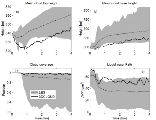
Figure 2 shows the evolution of the mean cloud top height, the mean cloud base height, the cloud coverage and the liquid water path from the master ensemble and

5

for 3DCLOUD during the 4 h simulations. Even though we can notice slight discrepan-cies between 3DCLOUD and master ensemble results in the first 2 h (“spinup” period), 3DCLOUD results are quite consistent with master ensemble results, especially at the end of the simulation. Nevertheless, 3DCLOUD tends to generate a lower cloud height than the mean results with a higher liquid water path.

10

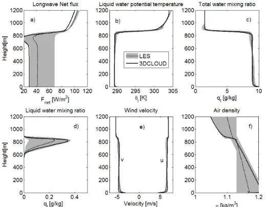
Figure 3 shows the mean profiles averaged over the fourth hour of the longwave net flux, the liquid water potential temperature, the total water mixing ratio, the liq-uid water mixing ratio, the horizontal velocity components, and the air density. Even though the 3DCLOUD longwave net flux is smaller compared to master ensemble, again 3DCLOUD results are quite consistent with others results for all the variables.

15

3.2 BOMEX (GCSS-WG1) case

For the BOMEX case (Siebesma et al., 2003), it was asked to perform a 6 h simulation on a horizontal grid of 64 by 64 points with 100 m spacing between grid node. Vertical spacing was required to be 40 m. In 3DCLOUD, we set thusNx=Ny =64 andNz=76

with Lx=Ly =6.4 km and Lz=2980 m, so ∆x= ∆y=100 m and ∆z≈39.2 m. Initial

20

profiles of the liquid water potential temperatureθl and the total water mixing ratioqt and the others required forcing including geostrophic winds, divergence due to the sub-sidence, surface sensible heat flux, surface latent heat flux, momentum surface fluxes, moisture large scale horizontal advection term and longwave radiative cooling (radia-tive effects due to the presence of clouds are neglected) are presented in Appendix B

25

(20)

GMDD

7, 295–337, 2014

cloud generator

F. Szczap et al.

Title Page

Tables Figures

◭ ◮

Back Close

Full Screen / Esc

Discussion

P

a

per

|

D

iscussion

P

a

per

|

Discussion

P

a

per

|

Discuss

ion

P

a

per

|

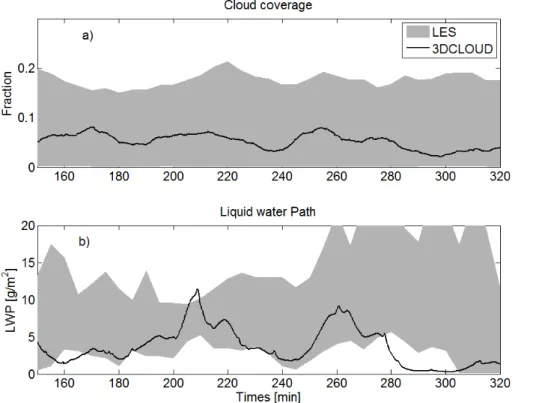
Figure 4 shows the evolution of the cloud coverage and the liquid water path from the master ensemble and for 3DCLOUD during the 6 h simulation. We can notice the small value of the cloud coverage (less than 10 %). 3DCLOUD results are quite consistent with the master ensemble results, even if the simulated 3DCLOUD liquid water path (LWP) may be too low at the end of the simulation.

5

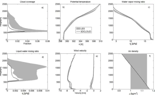
Figure 5 shows mean profiles averaged over the fifth hours of the cloud coverage, the potential temperature, the water vapour mixing ratio, the liquid water mixing ratio, the horizontal velocity components, and the air density. The 3DCLOUD results are again quite consistent with the master ensemble results. We note however that the 3DCLOUD cloud coverage and liquid water mixing ratio are smaller at any height. We also see

10

small di_fferences (less than 1 m s−1) for the wind velocity for height smaller than 500 m, for the potential temperature (less than 1 K) and for the water vapour mixing ratio (less than 1 g kg−1) for height larger than 1800 m.

3.3 ICMCP (GCSS-WG2) case

For the cirrus case detailed in Starr et al. (2000), the baseline simulations include

night-15

time “warm” cirrus and “cold” cirrus cases where cloud top initially occurs at₋47◦C and

−66◦C, respectively. The cloud is generated in an ice super-saturated layer with a ge-ometric thickness around 1 km (120 % in 0.5 km layer) and with a neutral ice pseudo-adiabatic thermal stratification. Cloud formation is forced via an imposed diabatic cool-ing over a 4 h time span followcool-ing by 2 h dissipation stage without coolcool-ing. All models

20

simulate radiative transfer, contrary to 3DCLOUD. In 3DCLOUD, we setNx=Ny =60

and N_z=140 with L_x=L_y =6.3 km and L_z=14 km, so that ∆x= ∆y=105 m and

∆z_≈100 m.

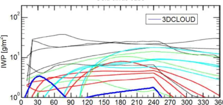
Figure 6 shows the evolution of the ice water path (IWP) from the master ensem-ble and for 3DCLOUD during the 6 h simulation. In a general way, most of the tested

25

models and 3DCLOUD have similar behaviour: indeed, the IWP increases during the first 4 h simulation (cirrus formation due to imposed cooling) and decreases after (cir-rus dissipation due to no imposed cooling). The IWP range of the tested models is

(21)

GMDD

7, 295–337, 2014

cloud generator

F. Szczap et al.

Title Page

Tables Figures

◭ ◮

Back Close

Full Screen / Esc

Discussion

P

a

per

|

D

iscussion

P

a

per

|

Discussion

P

a

per

|

Discuss

ion

P

a

per

|

very large (factor of 10), but we can notice that 3DCLOUD behaviour is closer to bulk microphysics models behaviours, especially for “warm cirrus”.

For “cold” cirrus, the 3DCLOUD IWP is smaller than most of participating models during all the simulation duration. It is probably because 3DCLOUD do not account for the radiative transfer as opposed to the participating models. Indeed, neglecting cirrus

5

top cooling due to radiative processes restricts the formation of the thin “cold” cirrus. This radiative diabatic effect is probably less important for the “warm” cirrus because the latent heat diabatic effect is larger.

4 Examples of 3DCLOUD possibilities

In this section, we present cloud fields generated by 3DCLOUD with the assimilation

10

of idealized meteorological profiles and fractional cloud coverage defined by the user. We also show the effect of the outer scale Lout and the inhomogeneity parameter of optical depthρτon the generated optical depth field. We also give an example of cirrus

clouds with fallstreaks. In order to have a spatial representation of the clouds as seen from above, we choose to show the so-called pseudo-albedoα defined as:

15

α= (1−g)τ

2₊(1₋g)τ (23)

where the asymmetry parametergis set to 0.86 andτis the optical depth.

4.1 Stratocumulus and cumulus fields with assimilation of meteorological profiles based on DYCOMS2-RF01 and BOMEX cases

We choose to simulate stratocumulus and cumulus LWC in the context of

DYCOMS2-20

(22)

GMDD

7, 295–337, 2014

cloud generator

F. Szczap et al.

Title Page

Tables Figures

◭ ◮

Back Close

Full Screen / Esc

Discussion

P

a

per

|

D

iscussion

P

a

per

|

Discussion

P

a

per

|

Discuss

ion

P

a

per

|

these profiles have to be slightly modified. At sea surface (z=0), for stratocumulus (DYCOMS2-RF01 case), the liquid potential temperature and total mixing ratio are set to 290 K and 10 g kg−1, respectively (instead of 289 K and 9 g kg−1, respectively). For cumulus (BOMEX case), the liquid potential temperature is set to 299.7 K instead of 298.7 K. In addition, wind profiles assimilated by 3DCLOUD are those computed by

5

the master ensemble at the end of simulation.

4.1.1 E_ffects of numerical spatial resolution

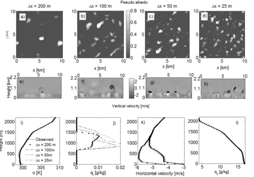
The effects of the numerical spatial resolution effects on 3DCLOUD simulations are presented here. Figure 7 shows pseudo-albedo and cross sections of the vertical ve-locity and cloud water at the end of the simulation for the stratocumulus case based

10

on the DYCOMS2-RF01 experiment. It also shows the mean profiles of potential tem-perature, liquid water mixing ratio, horizontal velocity components, and vapour water mixing ratio for different numerical spatial resolutions ∆x= ∆y=200 m, 100 m, 50 m and 25 m. Horizontal extensions L_x=L_y are set to 10 km and vertical resolution ∆z to 24 m for all simulations. Figure 8 is the same as Fig. 7, but for the cumulus case

15

with assimilation of meteorological profiles based on the BOMEX case. The vertical resolution∆z is set to 38.5 m in this last case.

It is obvious that change in the horizontal mesh leads to a more pleasant and detailed flow visualization but there is no significant impact on the mean statistics of the simu-lated temperature vertical profile, water vapour mixing ration and wind velocity. The

wa-20

ter mixing ratio simulated by 3DCLOUD for the DYCOMS2-RF01 case is very close to the mean profile averaged over the fourth hour and provided by master ensemble, even if the vertical resolution used in this section is only∆z=38.5 m compared to∆z=5 m in Sect. 3.1. For BOMEX case, the water mixing ratio simulated by 3DCLOUD changes as a function of numerical spatial resolution. This behaviour is quite understandable

25

as results drawn on Figs. 7 and 8 are snapshots at the end of the 3DCLOUD simu-lation and not average results over 1 h as done on Figs. 3 and 5. Moreover, BOMEX

(23)

GMDD

7, 295–337, 2014

cloud generator

F. Szczap et al.

Title Page

Tables Figures

◭ ◮

Back Close

Full Screen / Esc

Discussion

P

a

per

|

D

iscussion

P

a

per

|

Discussion

P

a

per

|

Discuss

ion

P

a

per

|

meteorological conditions cause time dependent cumulus fields, contrary to DYCOMS2 meteorological conditions that cause more stationary stratocumulus fields.

Although sensible and latent heat are not prescribed correctly and no radiative trans-fer scheme is used, 3DCLOUD is able to simulate correctly pertinent cloud statistics, such as temperature, water vapour mixing ratio, wind velocity and in particular cloud

5

water mixing ratio of stratocumulus and cumulus fields, given that the initial meteoro-logical profiles prescribed by the user are representative of the simulated cloud.

4.1.2 Assimilation of the fractional cloud coverageC

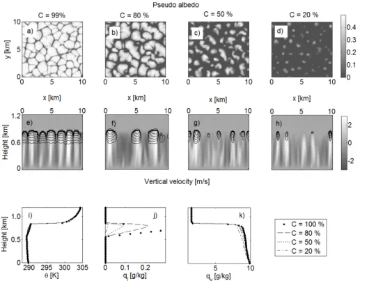
Results shown in Fig. 9 are the same results as Fig. 7 with in addition the assimilation of the cloud coverageC=99 %,C=80 %,C=50 % andC=20 %. Horizontal extensions

10

LxandLy are set 10 km and vertical resolution∆zis set to 24 m.

They show that 3DCLOUD is able to assimilate correctly fractional cloud coverage of stratocumulus for very different values ofC, even though the extreme example with C=20 % is a fair weather cumulus field rather than a stratocumulus. For each value of assimilatedC, it is interesting to note that cloud base and cloud top heights are still

15

localised around 600 m and 800 m, respectively. Temperature vertical profiles are al-most unchanged. The water mixing ratio vertical profiles decrease with the assimilated Cvalue.

4.1.3 Effect of the outer scaleL_outand inhomogeneity parameterρτ on the

optical depth field

20

We saw that 3DCLOUD can, at the end of the step 1, simulate stratocumulus and cu-mulus fields with enough coherent statistics profiles. However, optical depth (for stra-tocumulus and cumulus) or IWC (for cirrus) generated in the step 1 of 3DCLOUD does not show scale invariant properties observed in real cloud and often characterised by the spectral exponentβ1-D close to−5/3. As described in Sect. 2.2, it is the main task

25

(24)

GMDD

7, 295–337, 2014

cloud generator

F. Szczap et al.

Title Page

Tables Figures

◭ ◮

Back Close

Full Screen / Esc

Discussion

P

a

per

|

D

iscussion

P

a

per

|

Discussion

P

a

per

|

Discuss

ion

P

a

per

|

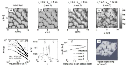
deviation of optical thickness or IWC. We focus on DYCOMS2-RF01 case at the reso-lution∆x=50 m (Fig. 7c). The effective radius Reff is set to 10 µm to compute optical depth from liquid water content. The mean optical depth of this initial field is set to 10 and we change the inhomogeneity parameterρτand the outer scaleLout, respectively, to 0.2 and 1 km for case 1, to 0.7 and 1 km for case 2 and to 0.7 and 10 km for case 3.

5

Figure 10 shows pseudo-albedo, mean power spectra, probability density function of optical depth fields, mean vertical profiles of the horizontally averaged optical depth for the three cases and a volume rendering of optical depth.

First, we notice that the pseudo-albedo of the initial optical depth field (see Fig. 10a) is smoother than the pseudo-albedo of case 1, 2, and 3. Between case 1 and 2, we see

10

clearly an increase of the heterogeneity as case 1 is a quasi-homogenous stratocumu-lus with a small value ofρ_τ=0.2 and case 2 is more inhomogeneous with a larger value ofρ_τ=0.7. Between case 2 and 3, we can see the effect of the outer scale. In accordance with smooth variation, the spectral slope of the initial optical depth is close to−3 for the [10−3: 10−2] m−1 wavenumber range (Fig. 10e). Case 1, 2 and 3 present

15

the proper spectral slope value of ₋5/3. For case 1 and 2, this slope is obtained for the [10−3: 10−2] m−1wavenumber range, which is coherent with the imposed value of outer scaleLout=1 km. For case 3,Lout=10 km, so the spectral slope should be−5/3 on the [10−4: 10−2] m−1wavenumber range, however we note that this spectral slope value is achieved only for the [5_×10−3: 10−2] m−1 wavenumber range. This is due to

20

the fact that we keep unchanged phase angles in the algorithm of 3DCLOUD.

In Fig. 10f, we represent the optical depth distributions. The initial optical depth dis-tribution does not follow common disdis-tribution, whereas the disdis-tribution of optical depth for case 1 and 2 are log-normal. Indeed, in the 3DCLOUD algorithm, we imposed a gamma distribution on optical depth. For case 2 and 3, optical depth distribution are

25

very close together, even if the outer scale are di_fferent. ChangingLoutvalue does thus not affect a lot the optical depth distribution shape. In Fig. 10g, we can see that the horizontal mean optical depth profiles are quasi identical for all cases.

(25)

GMDD

7, 295–337, 2014

cloud generator

F. Szczap et al.

Title Page

Tables Figures

◭ ◮

Back Close

Full Screen / Esc

Discussion

P

a

per

|

D

iscussion

P

a

per

|

Discussion

P

a

per

|

Discuss

ion

P

a

per

|

These results show undeniably the flexibility of the 3DCLOUD algorithm. Indeed, in step 2, 3DCLOUD is able, by mapping a theoretical gamma-distributed optical depth onto the optical depth field simulated at step1, to adjust, quasi-independently, the op-tical depth mean value, the inhomogenenity parameter value of opop-tical depth and the spectral slope value of optical depth for [1/Lout: 1/2∆x] m−

1

wavenumber range.

5

4.2 Cirrus fields with assimilation of idealized meteorological profiles

Including some modifications presented in this Sect. 2.1.1, 3DCLOUD is also able to generate cirrus cloud. We briefly present in this section an example of ice water content (IWC) of cirrus with fallstreaks. For cirrus, we chose to generate IWC field instead of optical depth field as for stratocumulus or cumulus.

10

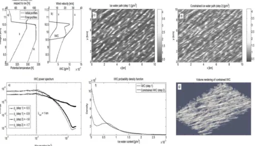
Figure 11 shows idealized vertical profiles of the potential temperature, the relative humidity, the horizontal velocity components assimilated by 3DCLOUD and the ice water path (IWP) simulated at step 1 by 3DCLOUD. It also shows the IWP simulated by 3DCLOUD during step 2, the initial and corrected mean power spectra, the initial and corrected probability density function and the IWC volume rendering. Horizontal

15

extensionsL_x=L_y and vertical extensionL_zare set to 10 km and 12.5 km, respectively. Horizontal resolutions∆x= ∆y and vertical∆zare set to 24 m and 83.3 m, respectively. IWC is set to 0.54 mg m−3, the value obtained at the end of step1. The inhomogeneity parameterρIWCis set to 1.0 and the outer scaleLoutis to 1 km.

Initial meteorological profiles assimilated by 3DCLOUD have been constructed in

20

such a way that thin cirrus is generated between 9.5 km and 10.5 km with fallstreaks. Vertical profiles of potential temperature, and especially their vertical gradients un-der and above the cirrus are based on those proposed by Liu et al. (2003). In orun-der to generate instabilities due to radiative cooling that is not simulated by 3DCLOUD, we imposed a null vertical gradient of the potential temperature near the cirrus top

25

(26)

GMDD

7, 295–337, 2014

cloud generator

F. Szczap et al.

Title Page

Tables Figures

◭ ◮

Back Close

Full Screen / Esc

Discussion

P

a

per

|

D

iscussion

P

a

per

|

Discussion

P

a

per

|

Discuss

ion

P

a

per

|

under the cirrus, RHI decreases with height to 85 % near 8 km. To generate fallstreaks, we imposed larger wind shear inside the cirrus than under the cirrus.

On Fig. 11, we note that IWP obtained after the step 1 is smoother than IWP af-ter the step 2, and that the initial IWC spectral slope value afaf-ter step 1 is much smaller (around−5.5) than the corrected IWC spectral slope after the step 2 (around

5

−1.6) in the [10−3: 2_×10−2] m−1 wavenumber range. For wavenumber smaller than 1/L_out=10−3m−1, the power spectra are constant. The corrected IWC probability is exponential-like distribution for step 2. It is due to the larger value ofρIWC=1.0 used in this example, compared toρ_τ=0.7 used for stratocumulus in Sect 4.1.3.

5 Conclusions

10

3DCLOUD is a flexible three-dimensional cloud generator developed to simulate with a personal computer and under Matlab environment, synthetic but realistic stratocu-mulus, cumulus and cirrus cloud fields. Simplified dynamic and thermodynamic laws allow the generation of realistic liquid or ice water content from meteorological pro-files. Stochastic process with Fourier framework allows us to provide ice water content

15

or optical depth sharing statistical properties with real clouds such as the inhomo-geneity parameter (set by the user) and the invariant scale properties characterised by a spectral slope close to₋5/3 from the smaller scale (set by spatial resolution of grid computation) to the outer scale (set by the user). In order to simulate cloud structure, 3DCLOUD solves the simplified basic atmospheric equations and assimilates the cloud

20

coverage set by the user (only for stratocumulus and cumulus regime) and meteoro-logical profiles (pressure, humidity, wind velocity) defined by the user.

The 3DCLOUD outputs were compared to the LES outputs for three classical test cases. We chose the case of DYCOMS2-RF01 (the first Research Flight of the sec-ond Dynamics and Chemistry of Marine Stratocumulus) for the marine stratocumulus

25

regime (Stevens et al., 2005), the case of BOMEX (Barbados Oceanographic and Me-teorological Experiment) for the shallow cumulus regime (Siebesma et al., 2003), and

(27)

GMDD

7, 295–337, 2014

cloud generator

F. Szczap et al.

Title Page

Tables Figures

◭ ◮

Back Close

Full Screen / Esc

Discussion

P

a

per

|

D

iscussion

P

a

per

|

Discussion

P

a

per

|

Discuss

ion

P

a

per

|

the case of ICMCP (Idealized Cirrus Model Comparison Project) for cirrus regimes (Starr, 2000). For these cases, results show that 3DCLOUD outputs are relatively con-sistent with LES outputs, and let us confirm that the chosen basic atmospheric equa-tions of 3DCLOUD are solved correctly. We also show that, under the condition that the user provides coherent meteorological profiles for the cloud to be simulated, 3DCLOUD

5

algorithm is able to assimilate them and generate realistic cloud structures.

3DCLOUD is a great tool to understand 3-D interactions between cloudy atmosphere and atmospheric radiation, in order to make progress in the direct radiative problem (GCM context) and in the inverse radiative problem (remote sensing context, develop-ment of next generation of atmospheric sensor). For example, 3DCLOUD was used

10

to quantify the impact of stratocumulus heterogeneities on polarized radiation mea-surements performed by POLDER/PARASOL (Cornet et al., 2013) as well as the influ-ence of cirrus heterogeneities on brightness temperature measured by IIR/CALIPSO (Fauchez et al., 2013).

We still have to develop into 3DCLOUD stochastic process to generate 3-D field of

15

cloud effective radius. In a longer term, investigations will focus on the generation of 3-D mixed phase cloud and eventually on the simulation of 3-3-D rain rate. Another task will be to provide a FORTRAN code of 3DCLOUD, assumed to be faster than the current Matlab code.

6 Code availability

20

The source code of the 3DCLOUD algorithm is available online at http://wwwobs. univ-bpclermont.fr/atmos/fr/restricted. Please contact authors for the password.

Acknowledgements. This work has been supported by the Programme Na-tional de Télédétection Spatiale (PNTS, http://www.insu.cnrs.fr/actions-sur-projets/ pnts-programme-national-de-teledetection-spatiale), grant no. PNTS-2012-08 and by the

25