www.atmos-meas-tech.net/7/4223/2014/ doi:10.5194/amt-7-4223-2014
© Author(s) 2014. CC Attribution 3.0 License.
Extending the satellite data record of tropospheric ozone profiles
from Aura-TES to MetOp-IASI: characterisation of optimal
estimation retrievals
H. Oetjen1,2, V. H. Payne2, S. S. Kulawik2,3, A. Eldering1,2, J. Worden2, D. P. Edwards4, G. L. Francis4, H. M. Worden4, C. Clerbaux5,6, J. Hadji-Lazaro5, and D. Hurtmans6
1The UCLA/JPL Joint Institute for Regional Earth System Science and Engineering, Los Angeles, California, USA 2Jet Propulsion Laboratory, California Institute of Technology, Pasadena, California, USA
3BAER Institute, Sonoma, California, USA
4National Center for Atmospheric Research, Boulder, Colorado, USA
5Sorbonne Universités, UPMC Univ. Paris 06; Université Versailles St-Quentin; CNRS/INSU, LATMOS-IPSL, Paris, France 6Spectroscopie de l’atmosphère, Service de Chimie Quantique et Photophysique, Université Libre de Bruxelles,
Brussels, Belgium
Correspondence to:H. Oetjen ([email protected])
Received: 4 June 2014 – Published in Atmos. Meas. Tech. Discuss.: 16 July 2014 Revised: 4 October 2014 – Accepted: 5 November 2014 – Published: 8 December 2014
Abstract.We apply the Tropospheric Emission Spectrome-ter (TES) ozone retrieval algorithm to Infrared Atmospheric Sounding Instrument (IASI) radiances and characterise the uncertainties and information content of the retrieved ozone profiles. This study focuses on mid-latitudes for the year 2008. We validate our results by comparing the IASI ozone profiles to ozone sondes. In the sonde comparisons, we find a negative bias (1–10 %) in the IASI profiles in the lower to mid-troposphere and a positive bias (up to 14 %) in the up-per troposphere/lower stratosphere (UTLS) region. For the described cases, the degrees of freedom for signal are on av-erage 3.2, 0.3, 0.8, and 0.9 for the columns 0 km – top of atmosphere, (0–6), (0–11), and (8–16) km, respectively. We find that our biases with respect to sondes and our degrees of freedom for signal for ozone are comparable to previously published results from other IASI ozone algorithms. In ad-dition to evaluating biases, we validate the retrieval errors by comparing predicted errors to the sample covariance ma-trix of the IASI observations themselves. For the predicted versus empirical error comparison, we find that these errors are consistent and that the measurement noise and the inter-ference of temperature and water vapour on the retrieval to-gether mostly explain the empirically derived random errors. In general, the precision of the IASI ozone profiles is better than 20 %.
1 Introduction
Ozone acts as a toxic pollutant in the lower troposphere, a greenhouse gas in the upper troposphere and a protec-tive shield against harmful ultraviolet (UV) radiation in the stratosphere. Information on the vertical distribution of ozone is therefore critical to understanding its impact on air quality, chemical composition and climate. Rapidly in-creasing Asian emissions of ozone precursors, land surface changes from burning and decreasing surface emissions in Europe and North America are resulting in ongoing changes to the spatial distribution of tropospheric ozone, which have yet to be well quantified (e.g. Wild and Akimoto, 2001; Fry et al., 2012). Satellite-borne measurements provide the means for global and continuous monitoring of this important trace gas.
Fu et al., 2013). However, in this work, we focus on ozone retrievals from the TIR.
Tropospheric Emission Spectrometer (TES), a Fourier transform spectrometer (FTS) on the Aura satellite, flying since 2004, was specifically designed with a focus on map-ping the global distribution of tropospheric ozone (Beer, 2006). The extremely high spectral resolution (0.1 cm−1
apodised) of the TES instrument enables profiling of tropo-spheric ozone. Aura-TES is in a sun-synchronous polar orbit with an equator overpass local time of ∼01:45 and 13:45. It makes nadir observations with a spatial resolution of 5.3 by 8.3 km. Successive orbit tracks are separated by about 22◦longitude. In the nominal TES observation mode, obser-vations are separated by 182 km along the flight track. The TES retrieval algorithm uses an optimal estimation approach (Bowman et al., 2006), which allows straightforward char-acterisation of the retrieval errors and the vertical sensitivity of the retrievals. The ozone product has been subject to on-going improvements over the years. A number of validation studies have demonstrated the quality of the TES radiances (Shephard et al., 2008; Connor et al., 2011), ozone profile re-trievals (Worden et al., 2007; Nassar et al., 2008; Verstraeten et al., 2013) and ozone retrieval error estimates (Boxe et al., 2010). The Boxe et al. (2010) study utilised special obser-vations from TES (“stare” mode) in order to obtain multiple observations of the same air mass, from which a covariance matrix could be constructed.
The capability to retrieve ozone profile information has also been demonstrated using radiance measurements from other TIR nadir sounders, such as the Interferometric Mea-surement of Greenhouse gases (IMG, e.g. Coheur et al., 2005) on ADEOS, the Atmospheric InfraRed Sounder (AIRS, e.g. Bian et al., 2007) on Aqua, the Infrared At-mospheric Sounding Instruments (IASI, e.g. Dufour et al., 2012) on the MetOp-A and -B satellites, the TANSO-FTS (Ohyama et al., 2012) on GOSAT, and the Cross-track In-frared Sounder (CrIS) on Suomi NPP (Han et al., 2013). Combining data sets with well-characterised sensitivity and uncertainty estimates can potentially provide the means to generate a consistent long-term record of tropospheric ozone that could be used in chemical composition and climate ap-plications.
In addition to the IASI instruments on MetOp-A and -B, an identical instrument will fly on the MetOp-C satellite, due to launch in 2017/18. Furthermore, EUMETSAT (Eu-ropean Organisation for the Exploitation of Meteorological Satellites) is currently preparing the next polar-orbiting pro-gramme with the Metop Second Generation (SG) satellite se-ries that should be launched around 2020. In this framework, studies are underway for the concept of a new instrument, the IASI-New Generation (IASI-NG), characterised by an im-provement of both spectral resolution and radiometric char-acteristics as compared to IASI (Clerbaux and Crevoisier, 2013). The IASI/IASI-NG data record is therefore of particu-lar interest in the context of quantifying long-term changes in
tropospheric ozone. In addition, the IASI instruments, unlike TES, provide swath coverage, allowing near-coincident ob-servations of the atmospheric state and enabling comparison between predicted and actual retrieval errors.
In this work, we apply the TES ozone retrieval algorithm to radiances from IASI on MetOp-A as a first step towards the goal of creating a consistent long-term record of tro-pospheric ozone from multiple TIR instruments (while this study is concerned with TES and IASI, instruments such as AIRS and CrIS also have potential to contribute information to such a record). This study concentrates on mid-latitudes in 2008 in order to facilitate comparison of our results with other IASI ozone retrievals as presented in the study by Du-four et al. (2012). The focus of this study is the characteri-sation and validation of the error estimates on the ozone re-trievals produced with this algorithm.
Section 2 gives the technical details of the IASI instru-ment. In Sect. 3, a summary of existing IASI ozone retrievals is given, while Sect. 4 describes the retrieval of ozone pro-files with optimal estimation theory and the theoretical tools for the characterisation of the profiles used in this study. In Sect. 5, an overview of the different reference data sets for validation is provided, followed by the results in Sect. 6.
2 The IASI instrument on MetOp-A
The IASI instrument is an FTS based on the Michelson inter-ferometer. 8461 channels cover a spectral range between 645 and 2760 cm−1with a resolution of 0.5 cm−1(after
apodisa-tion). The spectral sampling interval is 0.25 cm−1. IASI was
designed by the Centre National d’Études Spatiales (CNES) (Cayla, 1993; Blumstein et al., 2004) and launched in Octo-ber 2006 onboard the MetOp-A satellite. The mission is op-erated by EUMETSAT. Operational measurements have been performed since June 2007.
IASI flies on MetOp-A at an altitude of 817 km in a po-lar sun-synchronous orbit. The local overpass times at the equator are 09:30 and 21:30. MetOp-A completes slightly over 14 orbits a day. IASI is a nadir-viewing instrument and scans across the track within±48.3◦in a step and stare mode. There are 30 scans per swath. These 30 individual effective fields of view (EFOVs) are made up of four instantaneous fields of view (IFOVs) arranged in a 2×2 pixel matrix re-sulting in 120 measurements per scan line. The surface foot-print of a nadir IFOV is circular, of 12 km diameter. Towards the edge of the swaths, the IFOVs are elliptically elongated to a footprint of 20 km×39 km. A swath spans 2200 km in width. Global coverage is achieved twice daily.
in-tegrated ozone, carbon monoxide, nitrous oxide, methane, carbon dioxide, three partial columns of ozone (between the surface and 6, 12, and 16 km altitude), surface temperature, cloud information, and profiles for temperature and water vapour. More technical details can be found in the EUMET-SAT IASI Level 2 Product Guide (http://oiswww.eumetsat. org/WEBOPS/eps-pg/IASI-L2/IASIL2-PG-0TOC.htm) and in Clerbaux et al. (2009). In this work, we have utilised EU-METSAT temperature, water vapour and surface temperature products in the retrieval input (Sect. 4.2). In addition, we have made use of the cloud fraction that is reported in the Level 2 product (Sect. 4.3).
3 Existing IASI ozone data products
A number of different groups have previously developed ozone retrieval algorithms for IASI. Operational processing of IASI ozone data for the Level 2 product is done by EU-METSAT with a neural network based approach (Schlüs-sel et al., 2005; August et al., 2012) and by the Cen-ter for Satellite Applications and Research (STAR), part of the NOAA Satellite and Information Service (NESDIS), with an iterative regularised least squares minimisation al-gorithm (Bian et al., 2007; Pittman et al., 2009). At LAT-MOS/ULB (Laboratoire Atmosphères, Milieux, Observa-tions Spatiales/Université Libre de Bruxelles), the FORLI (Fast Operational Retrievals on Layers for IASI) algorithm uses an optimal estimation approach (Hurtmans et al., 2012). In the future FORLI ozone profiles will be distributed by EUMETSAT with the Level 2 product. We compare our re-trievals to FORLI results (see Sects. 5.3 and 6.5).
Other non-operational ozone data products have been derived at LISA (Laboratoire Inter-universitaire des Sys-tèmes Atmosphériques, Universités Paris-Est Créteil et Paris Diderot, CNRS/INSU) applying an altitude-dependent Tikhonov-Phillips regularisation (Eremenko et al., 2008; Du-four et al., 2010) and at LA (Laboratoire d’Aérologie/OMP) utilising an optimal estimation approach using a priori con-straints (Barret et al., 2011).
Validation with and comparison to independent measure-ments of other IASI products have been performed (Boynard et al., 2009; Keim et al., 2009; Pittman et al., 2009; Viatte et al., 2011; Dufour et al., 2012; Pommier et al., 2012; Scan-nell et al., 2012; Gazeaux et al., 2013) and also comparison to models (Parrington et al., 2012). In general, these stud-ies focus on the determination of the bias and the correlation with respect to independent measurements and on the deter-mination of the information content. Only Keim et al. (2009) and Dufour et al. (2012) also studied the precision of the re-trievals.
4 TOE – TES optimal estimation
We apply an optimal estimation (OE) approach (Rodgers, 2000) following the TES algorithm to IASI Level 1c radi-ances. The optimal estimation approach minimises the cost function:
C= ky−L(x, b)k2 S−ε1
+zapriori−z2S−1
a (1)
in a non-linear Levenberg–Marquardt iterative scheme (Bow-man et al., 2006). Here,y is the measured radiance, a
dis-crete vector, related to the true stateLtrueby an additive noise
modelε:
y=Ltrue+ε. (2)
Lcan also be interpreted as an operator describing the
ra-diative transfer dependent on the atmospheric state. Hence
L(x, b)is the forward model of a specific state vectorxand
parametersbheld constant in the retrieval. The second term of Eq. (1) describes the difference between the a priori profile
zapriori and the retrieved statez. The retrieval is constrained
with the measurement noise covariance matrixSεand the co-variance matrices corresponding to the a priori profilesSa. 4.1 OE framework for the characterisation
of the retrievals
Several diagnostics can be derived to describe the quality and uncertainty of the retrieved atmospheric state: the Jacobian matrixKis an output of the radiative transfer model and rep-resents the sensitivity of the forward model towards changes in the retrieved state:
K=∂L(z)
∂z . (3)
The gain matrixGdescribes the sensitivity of the retrieved state towards changes in the measured radiances and can be calculated from
G=KTS−ε1K+S−a1 −1
KTS−ε1. (4)
The averaging kernel matrixAzzcan be calculated from the gain matrix and the Jacobian:
Azz=GK. (5)
The averaging kernels describe the sensitivity of the retrieval to the true state. Example averaging kernels for the IASI-TOE ozone retrieval are shown in Fig. 1. The trace of the averaging kernel matrix gives the degrees of freedom for sig-nal (DOFS) of the retrieval.
Figure 1.Averaging kernels and errors for selected locations. The
angle in the individual panels refers to the viewing angle of the IASI instrument and DOF to the degrees of freedom for signal.
coupling or cross-correlation between simultaneously re-trieved parameters, and the uncertainties associated with pa-rameters that are not included in the retrieval state vector (see Sect. 4.3 for more details). Mathematically, the error covari-ance can be described as a sum of four terms:
Sez=(Azz−I)Ss(Azz−I)T | {z }
smoothing
+GSεGT | {z }
noise
(6)
+XGKbSb(GKb)T | {z }
systematic
+XAxsSbaret(Axs)T | {z }
cross-state
+res
withIthe identity matrix. Systematic errors originate from parametersb, which are held constant in the retrieval, with Kb andSb their respective Jacobians and error covariance matrices. The cross-state errors are caused by the simulta-neous retrieval of other atmospheric parameters that are not the target. They can be derived from the cross-state part of the averaging kernel matrix Axs and the corresponding er-ror covariance matrixSbaret. The residual term res includes all
uncertainties not considered or unknown. The square root of
Figure 2.Three microwindows (red lines) used in the IASI-TOE
ozone retrieval overlaid onto the 9.6 µm ozone band (black line). Example corresponds to the Valentia Island averaging kernel exam-ple from Fig. 1.
the diagonal of Eq. (6) yields the uncertainty on the ozone profile.
4.2 Retrieval input
The TES forward model is described in Clough et al. (2006). Calculations of radiances and Jacobians are performed using a fixed pressure grid of 66 levels. The absorption parame-ters used in the forward model are pre-calculated using the Line-By-Line Radiative Transfer Model (LBLRTM) (Clough et al., 2005) and the TES_v1.4 line parameter database (http: //rtweb.aer.com).
As mentioned above, the IASI Level 1c radiances are ob-tained from NOAA CLASS. The measurement noise covari-ance matrixSε is a diagonal matrix with the diagonal ele-ments set according to the noise-equivalent spectral radiance (NESR). The NESR in the TIR ozone band around 9.6 µm has been estimated at 20 nW (cm2sr cm−1)−1 from a set
of representative spectra measured in orbit (Clerbaux et al., 2009).
Ozone profiles are retrieved simultaneously with water vapour profiles in the spectral windows 990–1031, 1040– 1049, and 1069–1072 cm−1. Figure 2 shows these three
spectral windows in relation to the TIR ozone band around 9.6 µm.
climato-logical monthly mean stratospheric and mesospheric ozone field from a 2005–2010 simulation from the Whole Atmo-sphere Chemistry–Climate Model (WACCM) model (Kinni-son et al., 2007). The a priori profiles for ozone are binned by months and by region in 10◦latitude and 60◦longitude steps. The a priori water vapour profiles are taken from the EUMETSAT operational Level 2 product.
The retrieval for ozone is performed on 26 levels and for water vapour on 18 levels. Those retrieval grids are strongly linked with the constraints. The a priori constraint matri-ces are altitude-dependent Tikhonov constraints (Kulawik et al., 2006). In this technique, the constraint is optimised for a specified a priori covariance, for which MOZART-3 was used (Brasseur et al., 1998). The ozone constraint matrices are binned into five latitude bands and the water vapour con-straint matrix is the same for all locations on the globe.
Atmospheric temperature profiles and skin temperature are not retrieved. These are set to the IASI EUMETSAT oper-ational Level 2 values. Other parameters that are not retrieved include the CO2 profiles created from a 2004 MATCH
(Model of Atmospheric Transport and Chemistry) model run (Nevison et al., 2008) and scaled by 1.0055 per year, the surface emissivity over land from the Zhou et al. (2011) monthly climatology and the emissivity over water from Wu and Smith (1997). The surface pressure is taken from the op-erational Level 2 data.
4.3 Sources of error in the TOE retrievals and quality control
Many factors contribute to the overall uncertainty of the re-trieved ozone profile. Uncertainties arise from parameters fixed to climatological values or auxiliary data sets. These include the temperature profile, trace gas profiles for interfer-ing species, surface temperature, surface pressure, and emis-sivity climatology. In theory, the contribution of these errors to the overall uncertainty can be calculated with the system-aticterm of Eq. (6). Uncertainties associated with the
atmo-spheric state are rather difficult to quantify since the true state and consequently the corresponding error covariance are un-known. The only other parameter retrieved besides the ozone profile is the water vapour profile, and we can calculate the error on the ozone profile caused by cross-correlation for this species with Eq. (6).
Further, possible contamination of an IASI scene with clouds can lead to errors if not considered in the retrieval. The approach taken to account for the influence of cloud in the TES products is described in Kulawik et al. (2006). However, in this study we have chosen to screen for clouds. IASI radiances were selected for cloud fractions smaller than 13 % from EUMETSAT’s Level 2 product (following Cler-baux et al., 2009) and then the retrievals were performed on individual IASI IFOVs assuming a cloud-free scene. This is different from the approach applied for the operational TES products where cloud parameters are retrieved and then
in-cluded in the radiative transfer simulations for the trace gas retrievals. We might expect that the presence of thin clouds could have some influence on the result. For example, Wass-mann et al. (2011) have shown that neglecting the presence of a cirrus cloud with an IR optical thickness of 0.1 and a cloud top at 10 km in the ozone retrievals can lead to errors in the ozone profile of up to 25 % in the troposphere.
An overview of the IASI instrument calibration is given in Hilton et al. (2012): the spectral calibration accuracy is δν/ν=2×10−6whereνis the frequency. The absolute
cal-ibration in brightness temperature is better than 0.35 K and it was shown that AIRS and IASI agree within 0.2 K. The NESR for IASI was estimated from the measured radiances themselves. The NESR should be a good representation of the random errors although over time instrument issues could change this value.
In Eq. (1), the radiance term of the cost function is solely constrained by the measurement noise covariance (see Sect. 4.1). However, differences between modelled and mea-sured radiances can also originate from uncertainties in the forward model with the covarianceSf. This adds an
addi-tional term ofGSfGT to Eq. (6).Sf contains contributions
from the discretisation and interpolation of atmospheric pro-files, and spectroscopic errors. The vertical grid in the TES forward model has been chosen to be fine enough to make discretisation errors negligible, and the difference between radiances from the TES forward model and LBLRTM are less than 0.1 % (Clough et al., 2006). The dominant errors in the modelling of clear-sky radiances arise from uncertainties in the spectroscopic parameters used as input to the line-by-line calculations (see, for example, Alvarado et al., 2013).
In order to remove unphysical results, such as oscillations in the profile, we remove profiles withχ2 larger than 1.3, which is calculated by
χ2= 1
n(y−L(x, b))S −1
ε (y−L(x, b))
, (7) withnbeing the number of elements in the radiance vectors
yandL(x, b). This is the only additional quality screening
besides the cloud filtering.
5 Validation data and selection criteria
We have validated the IASI-TOE ozone retrievals against independent measurements from ozone sondes for mid-latitudes in 2008. In addition to quantifying the overall bias relative to the sondes, we have focused here on validating the error estimates obtained from the optimal estimation frame-work.
sonde profiles, and (c) determining the range of the deviation from a mean of an ensemble of quasi-coinciding retrieved profiles, i.e. calculating the so-called sample covariance ma-trix. In the sample covariance approach, we assume that the true atmospheric ozone field is relatively constant over some limited spatial domain. For the IASI-TOE retrieval, which is primarily sensitive to ozone in the free troposphere (see Fig. 3), we assume that this spatial domain can extend over up to 10 IFOVs or about 220 km.
5.1 Ozone sondes
Ozone sonde profiles have been obtained from the World Ozone and Ultraviolet Data Centre (WOUDC, www.woudc. org) and from the Global Monitoring Division of NOAA (www.esrl.noaa.gov/gmd). The theoretical uncertainty of electrochemical concentration cell (ECC) sondes for a typ-ical mid-latitude ozone profile peaks at the ozone minimum (about 13 km) at about 9 % (WMO, 2011). However, the ab-solute uncertainty depends on various factors, e.g. the con-centration of the potassium iodide solution and the sonde preparation. Through laboratory studies for precision of the sondes as well as comparisons to UV-photometer ozone mea-surements, the accuracy is estimated to be 10 % or better for ECC sondes and 13 % or better for Brewer-Mast type sondes (only at Hohenpeißenberg) for the altitude range considered in the IASI-TOE comparison (WMO, 2011). In some cases, the WOUDC distributes a correction factor together with the sonde profiles. This correction factor is calculated from the ratio of a Brewer/Dobson instrument coincident total ozone measurement to the integrated ozone profile from the sonde plus a climatology above the burst height of the sounding balloon. Three different scenarios for soundings used in this study were encountered: (a) a correction factor was not given, (b) a correction factor was stated and applied to the sonde profile, and (c) a correction factor was stated, but not applied. For cases a and b we used the ozone profiles as given, but for case c we applied the factor to consolidate the measure-ments. Sondes with correction factors larger than 15 % were excluded from this study.
IASI scenes were selected to be within ±7 h and within a circle of 110 km (equivalent to 1◦latitude) radius around the sounding site following Dufour et al. (2012). These sites are listed in Table 1 together with the geolocation, elevation above sea level (a.s.l.) and the numbers of the soundings and of the IASI scenes.
In order to estimate the IASI-TOE retrieval’s limited verti-cal sensitivity, the averaging kernel matrixAzztogether with the a priori profilezaprioriis applied to the sonde profilezsonde
(Rodgers and Connor, 2003) to obtain a new profilezˆ mim-icking the IASI measurement:
ˆ
z=zapriori+Azz zsonde−zapriori
. (8)
p
ressu
re
[h
P
a]
Figure 3.Mean sums of rows of the averaging kernels separated by
season (southern hemispheric stations offset by 6 months). All IASI scenes as indicated in Table 1 are included.
We determine the mean bias of the IASI-TOE ozone profiles
zTOEi with respect to the ozone sonde profileszsondei :
¯
zsondebias= 1
N X
i
zTOEi −zsondei
(9)
= 1 N
X
i
zsondebiasi .
Note thatzsondei is not always unique if there is more than
one IASI scene fulfilling the coincidence criteria for the same sonde. The mean bias is a measure of the absolute accuracy of the retrievals, while the corresponding standard deviation σis a measure of the precision of the retrievals. Note that the fact that the sonde and the satellite are not viewing exactly the same air mass could make the standard deviation slightly larger than the true precision. The corrected sample variance σ2,correctedreferring to the degrees of freedom of (N−1), is
σ2= 1
N−1 X
i
zsondebiasi − ¯zsondebias
2
. (10)
The rms deviation (RMSD) can be calculated from
RMSD=
s 1 N
X
i
zTOEi −zsondei 2 (11)
Table 1.Locations with geoinformation and numbers of ozone sondes and IASI-TOE profiles, and mean DOFS.
Station (elevation above sea level) Latitude Longitude # of TOE scenes # of sondes DOFS
Goose Bay (36 m) 53.3◦N 60.4◦W 363 30 2.84
Legionowo (96 m) 52.4◦N 21.0◦E 158 19 3.31
Lindenberg (112 m) 52.2◦N 14.1◦E 238 29 3.24
Valentia Island (14 m) 51.9◦N 10.3◦W 367 32 3.15
Bratt’s Lake (580 m) 50.2◦N 104.7◦W 524 41 3.09
Prague (304 m) 50.0◦N 14.4◦E 191 27 3.03
Kelowna (456 m) 49.9◦N 119.4◦W 1240 62 3.10
Hohenpeißenberg (976 m) 47.8◦N 11.0◦E 688 80 3.17
Payerne (491 m) 46.5◦N 6.6◦E 851 93 3.20
Trinidad Head (20 m) 40.8◦N 124.2◦W 753 60 3.27
Madrid (631 m) 40.5◦N 3.6◦W 261 34 3.43
Boulder (1743 m) 40.0◦N 105.3◦W 230 38 3.32
Ankara (891 m) 40.0◦N 32.9◦E 214 19 3.21
Wallops Island (13 m) 37.9◦N 75.5◦W 513 36 3.38
Macquarie Island (6 m) 54.5◦S 158.9◦E 204 20 2.74
Ushuaia (17 m) 54.9◦S 68.3◦W 166 19 2.76
All – – 6961 639 3.16
5.2 Sample covariance matrix
The sample covariance matrix provides an estimate of the error covariance matrix: we havenobservationsz1...nof the random vectorZ. Then the sample covariance matrix is given
by
Q= 1 n−1
n X
i=1
(zi− ¯z) (zi− ¯z)T, (12)
wherez¯ is the sample mean. The degrees of freedom used here are (n−1) becausez¯does not equalZ. Here, the
mea-sured quantitiesz1...n, i.e. the retrieved ozone profiles, are not random with respect to the smoothing error because they all depend on the same a priori profile. Also other systematic er-rors cancel out since only relative differences are calculated. Consequently, the square root of the diagonal ofQis a mea-sure for the precision only. Note that Eq. (12) is equivalent to the variance of Eq. (10) if only one ozone sonde profile for the bias determination is used.
It is assumed that several retrieved ozone profiles of ad-jacent and concurrent IASI scenes are representative sam-ple measurements of the true ozone profile. This assumption is valid for ozone in the free troposphere and lower strato-sphere, the region of the atmosphere IASI is mostly sensitive to (see Fig. 3), and for a sufficiently large number of the sam-ple sizen. The same co-location criterion as above is applied, i.e. measurements within a circle with a radius of 110 km. In the best case, this results in about 64 scenes that could fulfil the co-location criterion. In addition to this, only IASI-TOE profiles from the same swath are used, guaranteeing the mea-surements to be within less than 38 s of each other. Here, the cloud fraction was limited to smaller than 6 %.
5.3 FORLI
A detailed description of the FORLI algorithm can be found in Hurtmans et al. (2012). Briefly, ozone profiles are re-trieved on a constant height grid with 1 km thick layers from the surface to 40 km altitude. The absorbance cross-sections are pre-calculated from the HITRAN database (Rothman et al., 2005). The spectral range is 1025–1075 cm−1. Only one
global ozone a priori profile and corresponding covariance matrix are used for all seasons. Just like for TOE, FORLI utilises the operational Level 2 temperatures and the water vapour profiles as input as well as the emissivity climatology by Zhou et al. (2011). Also, TOE and FORLI use the same value for the diagonal of the measurement noise covariance matrix, i.e. 20 nW (cm2sr cm−1)−1(Clerbaux et al., 2009).
IASI-FORLI ozone profiles were selected around the ozone sounding location with the same selection criteria as for IASI-TOE (although actual ozone sonde measurements were not included in this comparison). In general, since the retrieved ozone profiles undergo different quality screening, TOE and FORLI processing result in different subsets of successful profile retrievals for the same IASI scenes. For the comparison, we use a common subset. Since the two re-trievals use different a priori profiles, the IASI-TOE a priori profileszapriori(TOE)are swapped out with the IASI-FORLI a priorizapriori(FORLI)(Rodgers and Connor, 2003):
zFORLI aprioriTOE = (13)
zTOE+(Azz−I) zapriori(TOE)−zapriori(FORLI)
6 Results
Table 1 gives an overview of the number of IASI scenes that are used in this study. Overall, there are 6961 TOE retrievals that passed the various selection criteria (see Sects. 4.3 and 5.1) corresponding to 639 ozone soundings at 16 locations, two of which are in the Southern Hemisphere.
6.1 Vertical sensitivity of the IASI-TOE ozone retrievals Figure 3 shows the vertical distribution of the sum of the averaging kernel matrix rows split by season. Those are the means at the individual pressure levels and the correspond-ing 1σstandard deviation. Only between 300 and 700 hPa the values differ slightly with the season. Highest values are ob-served for summer (JJA) and lowest for winter (DJF). Also shown are the statistics for the DOFS for the different sea-sons for selected partial columns, and those follow the same seasonal trend (see Fig. 4). The overall mean DOFS for the total column are 3.2 (see Table 1). The DOFS for the par-tial columns in the troposphere (0–11 km) and in the upper troposphere/lower stratosphere (UTLS; 8–16 km) are slightly lower than 1 in summer. The whiskers in Fig. 4 represent the maximum and minimum values. Interestingly, the largest maximum values can be found for the winter partial columns (0–6, 0–11, 8–16 km) adding more than half a DOFS to the tropospheric partial columns in the extreme case. This indi-cates that not only the thermal contrast determines the DOFS, but also the low humidity in winter plays a role in the infor-mation content of the retrieval.
6.2 Theoretical error estimates
Figure 1 shows examples of IASI-TOE theoretical ozone retrieval errors and averaging kernels. These are examples for single ozone retrievals and not averages. The individ-ual errors are calculated with the different terms of Eq. (6),
smoothing andnoise as labelled and waterwith the cross-state term. The temperature error in Fig. 1 is calculated
somewhat differently: we estimate how the temperature er-ror propagates into the ozone profile with a temperature erer-ror covariance matrix derived from an ensemble of EUMETSAT Level 2 temperature profiles of quasi-coincident IASI scenes for these individual cases (Eq. 6),systematicterm). See also
Sects. 5.2 and 6.4. The sample size used for the calculation of the covariance is given in the label as n. The uncertain-ties are dominated by the smoothing error and peak at about 30 % in the lowest retrieval level. This reflects the limited sensitivity of the measurements as can also be seen in the av-eraging kernels. In the UTLS, the overall error is between 10 and 12 %. In the case of Bratt’s Lake, the averaging kernels do not decrease as rapidly towards the surface as in the other three examples due to a stronger thermal contrast (14 K vs. 4, 1, and 3 K for Valentia Island, Legionowo, and Wallops Island, respectively). Consequently, although the uncertainty
Figure 4.Bottom panel: statistics for DOFS for selected partial
columns as indicated in the legend, separated by season (southern hemispheric stations offset by 6 months). The boxes represent the 25th and 75th percentiles and the whiskers the minimum and max-imum values of the distribution. All IASI-TOE scenes as indicated in Table 1 are included. Top panel: sample size for calculating the statistics in the bottom panel. The overall sample size is 6961.
at the surface is the same as in the other cases, the uncertainty decreases more rapidly with height. This results in more in-formation on the tropospheric profile in this case, as indicated by the rather high number of 3.7 DOFS.
6.3 Biases relative to ozone sondes
The bias of IASI-TOE with respect to the ozone sonde pro-files is shown in Fig. 5 for the 16 individual locations as listed in Table 1. A clear picture emerges for all locations: a positive bias can be found in the UTLS region. Towards the surface the bias vanishes because of the limited sensitiv-ity of IASI there. From this figure it can be concluded that the biases and standard deviations of the TOE retrievals with respect to the sondes are similar for different locations, even though different kinds of ozone sondes, as well as different a priori profiles/constraints, were applied in the retrievals. Consequently in the following, the bulk quantities for all lo-cations together can be analysed.
Figure 5.Bias of the IASI-TOE profiles with respect to ozone sonde profiles separated by location. The numbers of profiles included are
indicated in the legend. The averaging kernels and ozone a priori profiles have been applied to the ozone sonde profiles. The coloured lines
show the individual biases, the black solid lines the means, and the dashed lines the 1σ standard deviations of the averaging. No significant
differences in the individual biases or standard deviations can be observed for the different locations.
raw ozone sonde data. As expected, the standard deviation is larger in this case since the variability of the ozone sonde measurements will be reduced due to the application of the averaging kernels (see also Fig. 7). In Fig. 7, the standard de-viation is plotted together with the rms dede-viation (see Eq. 11). The rms deviation is a measure for the precision and the bias error; the standard deviation is a measure for the precision only. As mentioned above, the bias error can be calculated from these quantities. When looking at the absolute numbers in Fig. 7, the following two points have to be kept in mind: (a) the estimates also include the precision of the ozone sonde (∼5 % for ECC sondes; WMO, 2011) and (b) the strength of the constraint of the retrieval is reflected in the precision, i.e.
a strong constraint will pull the retrieved profile towards the a priori profile, resulting in less scatter in the results.
6.4 Empirical vs. theoretical random errors
p
ressu
re
[h
P
a]
50
200
500
Figure 6.Bias of the IASI-TOE profiles with respect to the ozone sonde profiles. The number of profiles included are indicated in the legend.
The left panel shows the comparison after the averaging kernels (AK) and a priori profiles have been applied to the ozone sonde profiles (see Eq. 8). The right panel shows the comparison without the averaging kernels applied. The coloured lines indicate the individual biases, the
black solid lines the mean, and the dashed lines the 1σstandard deviations of the averaging.
Figure 7.The rms deviation, standard deviation of the mean bias,
and bias error of the IASI-TOE profiles with respect to raw ozone sonde profiles (solid lines) and after the averaging kernels (AK) have been applied (dashed lines). The standard deviation represents the precision of the IASI measurements (and also that of the ozone sondes) whereas the rms deviation is the square root of the sum of the squared precision and the squared bias.
variation in the retrieved ozone within the concurrent set of IFOVs (the empirical error) and the theoretical error calcu-lated using Eq. (6). Twelve of the 16 different sites had 15 or more concurrent ozone profiles and one example per site is shown in Fig. 8. The black lines are the square root of the diagonal of the sample covariance matrix calculated with Eq. (12) hereafter referred to as empirical error. The mag-nitude of the empirical error is similar to the theoretical er-ror (brown line). In general, (although not in all cases) the empirical errors are larger than the theoretical errors. Abso-lute differences are less than 11 %. The profile shape of the
Figure 8.Theoretical random errors (brown lines) and empirical
random errors (black lines) calculated from the square root of the
diagonal of the error covariance matrixQ(see Sect. 6.4) for selected
cases.
p
ressu
re
[h
P
a]
50
200
500
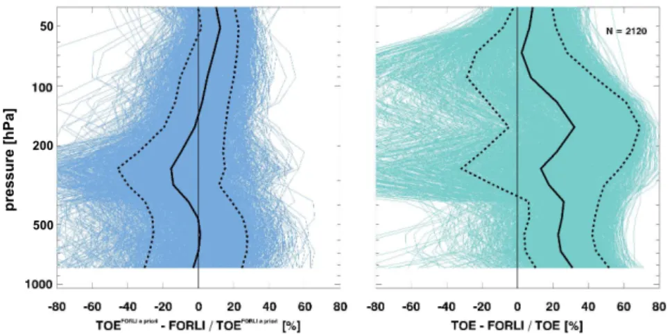
Figure 9.Bias of IASI-TOE profiles with respect to IASI-FORLI. The left panel shows the comparison after the TOE a priori profiles were
swapped out with the FORLI a priori profile; the right panel shows the comparison for the profiles without the averaging kernels applied. The
black lines represent the mean, the dashed lines the standard deviation, and the coloured lines are the differences of theN=2120 individual
profiles.
the individual IASI scenes within the coincidence area, but no outliers were detected. We also tested the standard de-viation of the individual theoretical errors for all the shown cases and it is smaller than 1 % for water vapour, smaller than 2 % for noise, and smaller than 2.5 % for the smoothing er-ror. Note that the remaining differences could reflect actual atmospheric variability or a too small sample size to obtain a representative sample covariance matrix.
For the presented cases, the empirical errors usually peak in the lower troposphere and the profile shape at sites with a large sample size (e.g. Kelowna and Ankara) is very sim-ilar to the profile shape of the mean standard deviation with respect to the ozone sondes as presented in Fig. 7. The empir-ical errors are smaller than 18 % and can be as low as 6 % in the UTLS region. These values also compare to the standard deviation of Fig. 7. Overall, it can be concluded that the ob-served variability is consistent with theoretical error budgets. 6.5 Comparison with IASI-FORLI
The comparisons between IASI-FORLI and IASI-TOE ozone profiles are shown in Fig. 9. The two retrievals agree within the 1σ-level when the IASI-TOE a priori profile has been modified to be the same as the IASI-FORLI a priori pro-file using Eq. (13) (Fig. 9, left panel). The particular shape of the bias between TOE and FORLI can be explained in terms of the biases of the respective retrieval profiles in compari-son to ozone compari-sondes. The FORLI positive bias towards ozone sondes (see Dufour et al., 2012) is positioned slightly lower than TOE’s. The differences between the two retrievals can be attributed to the differences in the ozone covariance matri-ces: FORLI uses a weaker constraint, but a larger correlation length for the retrieval levels in comparison to TOE/TES. In terms of the raw differences, the TOE retrieval results in larger ozone concentrations than FORLI at most levels (Fig. 9, right panel).
7 Summary of results and discussion
In this section the main findings are summarised and put into context.
– On average, the overall DOFS are 3.2 and the DOFS for the partial columns are 0.3, 0.8, and 0.9 for (0–6), (0–11), and (8–16) km, respectively. These numbers are similar to the numbers reported in Dufour et al. (2012) for three different IASI ozone retrievals, which include the FORLI retrieval.
– In general, the lower atmospheric DOFS as well as the overall DOFS are higher for warmer seasons (see Fig. 4).
– The theoretical error of the ozone profile is dominated by the smoothing error. The water vapour error plays only a minor role. The temperature profile error values and vertical distributions are quite variable and uncer-tainties can be as low as 3 %, but up to 20 % in some cases (see Figs. 1, 8). Overall, the error is about 30 % at the surface and decreases to about 10 ,% in the UTLS. – The empirical random errors are broadly consistent with
with theoretical errors for TES ozone retrievals (Boxe et al., 2010).
– The IASI-TOE ozone profiles show a positive bias in comparison to the ozone sonde profiles. The bias is greatest between 200 and 70 hPa when the averaging kernels are applied to the sonde profiles (Fig. 6, left panel). The maximum bias is 14 %. A positive bias has been observed before for IASI ozone profiles of three different retrievals (Dufour et al., 2012). This pos-itive bias is found for TES as well (e.g. Verstraeten et al., 2013), but also TANSO-FTS (Ohyama et al., 2012) and consequently the bias might be caused by incorrect spectroscopic parameters since it is independent from the observing system.
– FORLI and TOE ozone profiles are consistent with each other when the a priori profiles have been consolidated for the two retrievals (Fig. 9, left panel).
– When looking at the raw differences, the TOE retrieval results in larger ozone concentrations than FORLI at most levels (Fig. 9, right panel) as a result of the choice of a priori ozone values for FORLI versus TOE. It can be concluded that the IASI-TOE profile errors are consistent with other retrievals for IASI and TES and that the TOE ozone profiles are consistent with the IASI-FORLI profiles. Dedicated comparisons between IASI-TOE and TES ozone will be the topic of future work.
Acknowledgements. We acknowledge the NOAA/CLASS data
centre for the IASI Level 1c spectra and EUMETSAT for the Level 2 data. IASI is a joint mission of EUMETSAT and the Centre National d’Études Spatiales (CNES, France). The ozone sonde data were provided by the Global Monitoring Division of NOAA (www.esrl.noaa.gov/gmd) and by the World Ozone and Ultraviolet Data Centre (www.woudc.org). Part of the research was carried out at the Jet Propulsion Laboratory, California Institute of Technology, under a contract with the National Aeronautics and Space Administration. We acknowledge NASA support under the grant NNX11AE19G. We thank Gaëlle Dufour (LISA, France) for discussions.
Edited by: M. Weber
References
Alvarado, M. J., Payne, V. H., Mlawer, E. J., Uymin, G., Shephard, M. W., Cady-Pereira, K. E., Delamere, J. S., and Moncet, J.-L.: Performance of the Line-By-Line Radiative Transfer Model (LBLRTM) for temperature, water vapor, and trace gas retrievals: recent updates evaluated with IASI case studies, Atmos. Chem. Phys., 13, 6687–6711, doi:10.5194/acp-13-6687-2013, 2013. August, T., Klaes, D., Schlüssel, P., Hultberg, T., Crapeau, M.,
Arriaga, A., O’Carroll, A., Coppens, D., Munro, R., and Cal-bet, X.: IASI on Metop-A: Operational Level 2 retrievals after
five years in orbit, J. Quant. Spectrosc. Ra., 113, 1340–1371, doi:10.1016/j.jqsrt.2012.02.028, 2012.
Barret, B., Le Flochmoen, E., Sauvage, B., Pavelin, E., Matricardi, M., and Cammas, J. P.: The detection of post-monsoon tropo-spheric ozone variability over south Asia using IASI data, At-mos. Chem. Phys., 11, 9533–9548, doi:10.5194/acp-11-9533-2011, 2011.
Beer, R.: TES on the Aura mission: Scientific objectives, mea-surements, and analysis overview, IEEE T. Geosci. Remote, 44, 1102–1105, doi:10.1109/tgrs.2005.863716, 2006.
Bian, J. C., Gettelman, A., Chen, H. B., and Pan, L. L.: Validation of satellite ozone profile retrievals using Beijing ozonesonde data, J. Geophys. Res., 112, D06305, doi:10.1029/2006jd007502, 2007. Blumstein, D., Chalon, G., Carlier, T., Buil, C., Hebert, P., Ma-ciaszek, T., Ponce, G., Phulpin, T., Tournier, B., and Simeoni, D.: IASI instrument: technical overview and measured perfor-mances, SPIE Conference, Denver (CO), SPIE 2004-5543-22, August 2004.
Bowman, K. W., Rodgers, C. D., Kulawik, S. S., Worden, J., Sarkissian, E., Osterman, G., Steck, T., Lou, M., Eldering, A., Shephard, M., Worden, H., Lampel, M., Clough, S., Brown, P., Rinsland, C., Gunson, M., and Beer, R.: Tropospheric emis-sion spectrometer: Retrieval method and error analysis, IEEE T. Geosci. Remote, 44, 1297–1307, doi:10.1109/tgrs.2006.871234, 2006.
Boxe, C. S., Worden, J. R., Bowman, K. W., Kulawik, S. S., Neu, J. L., Ford, W. C., Osterman, G. B., Herman, R. L., Eldering, A., Tarasick, D. W., Thompson, A. M., Doughty, D. C., Hoff-mann, M. R., and Oltmans, S. J.: Validation of northern latitude Tropospheric Emission Spectrometer stare ozone profiles with ARC-IONS sondes during ARCTAS: sensitivity, bias and error analysis, Atmos. Chem. Phys., 10, 9901–9914, doi:10.5194/acp-10-9901-2010, 2010.
Boynard, A., Clerbaux, C., Coheur, P.-F., Hurtmans, D., Tur-quety, S., George, M., Hadji-Lazaro, J., Keim, C., and Meyer-Arnek, J.: Measurements of total and tropospheric ozone from IASI: comparison with correlative satellite, ground-based and ozonesonde observations, Atmos. Chem. Phys., 9, 6255–6271, doi:10.5194/acp-9-6255-2009, 2009.
Brasseur, G. P., Hauglustaine, D. A., Walters, S., Rasch, P. J., Müller, J. F., Granier, C., and Tie, X. X.: MOZART, a global chemical transport model for ozone and related chemical trac-ers 1. Model description, J. Geophys. Res., 103, 28265–28289, doi:10.1029/98jd02397, 1998.
Cayla, F.-R.: IASI infrared interferometer for operations and re-search, in: High Spectral Resolution Infrared Remote Sensing for Earth’s Weather and Climate Studies, edited by: Chedin, A., Chahine, M. T., and Scott, N. A., NATO ASI Series, I 9, Springer Verlag, Berlin-Heidelberg, 9–19, 1993.
Clough, S. A., Shephard, M. W., Mlawer, E., Delamere, J. S., Iacono, M., Cady-Pereira, K., Boukabara, S., and Brown, P. D.: Atmospheric radiative transfer modeling: a summary of the AER codes, J. Quant. Spectrosc. Ra., 91, 233–244, doi:10.1016/j.jqsrt.2004.05.058, 2005.
Clough, S. A., Shephard, M. W., Worden, J., Brown, P. D., Wor-den, H. M., Luo, M., Rodgers, C. D., Rinsland, C. P., Gold-man, A., Brown, L., Kulawik, S. S., Eldering, A., Lampel, M., Osterman, G., Beer, R., Bowman, K., Cady-Pereira, K. E., and Mlawer, E. J.: Forward model and Jacobians for Tropospheric Emission Spectrometer retrievals, IEEE T. Geosci. Remote, 44, 1308–1323, doi:10.1109/tgrs.2005.860986, 2006.
Coheur, P.-F., Barret, B., Turquety, S., Hurtmans, D., Hadji-Lazaro, J., and Clerbaux, C.: Retrieval and characterization of ozone ver-tical profiles from a thermal infrared nadir sounder, J. Geophys. Res., 110, D24303, doi:10.1029/2005jd005845, 2005.
Connor, T. C., Shephard, M. W., Payne, V. H., Cady-Pereira, K. E., Kulawik, S. S., Luo, M., Osterman, G., and Lampel, M.: Long-term stability of TES satellite radiance measurements, At-mos. Meas. Tech., 4, 1481–1490, doi:10.5194/amt-4-1481-2011, 2011.
Cuesta, J., Eremenko, M., Liu, X., Dufour, G., Cai, Z., Höpfner, M., von Clarmann, T., Sellitto, P., Foret, G., Gaubert, B., Beek-mann, M., Orphal, J., Chance, K., Spurr, R., and Flaud, J.-M.: Satellite observation of lowermost tropospheric ozone by mtispectral synergism of IASI thermal infrared and GOME-2 ul-traviolet measurements over Europe, Atmos. Chem. Phys., 13, 9675–9693, doi:10.5194/acp-13-9675-2013, 2013.
Dufour, G., Eremenko, M., Orphal, J., and Flaud, J.-M.: IASI observations of seasonal and day-to-day variations of tropo-spheric ozone over three highly populated areas of China: Bei-jing, Shanghai, and Hong Kong, Atmos. Chem. Phys., 10, 3787– 3801, doi:10.5194/acp-10-3787-2010, 2010.
Dufour, G., Eremenko, M., Griesfeller, A., Barret, B., LeFlochmoën, E., Clerbaux, C., Hadji-Lazaro, J., Coheur, P.-F., and Hurtmans, D.: Validation of three different scientific ozone products retrieved from IASI spectra using ozonesondes, Atmos. Meas. Tech., 5, 611–630, doi:10.5194/amt-5-611-2012, 2012.
Emmons, L. K., Walters, S., Hess, P. G., Lamarque, J.-F., Pfister, G. G., Fillmore, D., Granier, C., Guenther, A., Kinnison, D., Laepple, T., Orlando, J., Tie, X., Tyndall, G., Wiedinmyer, C., Baughcum, S. L., and Kloster, S.: Description and evaluation of the Model for Ozone and Related chemical Tracers, version 4 (MOZART-4), Geosci. Model Dev., 3, 43–67, doi:10.5194/gmd-3-43-2010, 2010.
Eremenko, M., Dufour, G., Foret, G., Keim, C., Orphal, J., Beek-mann, M., Bergametti, G., and Flaud, J. M.: Tropospheric ozone distributions over Europe during the heat wave in July 2007 ob-served from infrared nadir spectra recorded by IASI, Geophy. Res. Lett., 35, L18805, doi:10.1029/2008gl034803, 2008. Fry, M. M., Naik, V., West, J. J., Schwarzkopf, M. D., Fiore, A.
M., Collins, W. J., Dentener, F. J., Shindell, D. T., Atherton, C., Bergmann, D., Duncan, B. N., Hess, P., MacKenzie, I. A., Marmer, E., Schultz, M. G., Szopa, S., Wild, O., and Zeng, G.: The influence of ozone precursor emissions from four world re-gions on tropospheric composition and radiative climate forc-ing, J. Geophys. Res., 117, D07306, doi:10.1029/2011jd017134, 2012.
Fu, D., Worden, J. R., Liu, X., Kulawik, S. S., Bowman, K. W., and Natraj, V.: Characterization of ozone profiles derived from Aura TES and OMI radiances, Atmos. Chem. Phys., 13, 3445–3462, doi:10.5194/acp-13-3445-2013, 2013.
Gazeaux, J., Clerbaux, C., George, M., Hadji-Lazaro, J., Kuttippu-rath, J., Coheur, P.-F., Hurtmans, D., Deshler, T., Kovilakam, M., Campbell, P., Guidard, V., Rabier, F., and Thépaut, J.-N.: Inter-comparison of polar ozone profiles by IASI/MetOp sounder with 2010 Concordiasi ozonesonde observations, Atmos. Meas. Tech., 6, 613–620, doi:10.5194/amt-6-613-2013, 2013.
Han, Y., Revercomb, H., Cromp, M., Gu, D., Johnson, D., Mooney, D., Scott, D., Strow, L., Bingham, G., Borg, L., Chen, Y., DeSlover, D., Esplin, M., Hagan, D., Jin, X., Knuteson, R., Mot-teler, H., Predina, J., Suwinski, L., Taylor, J., Tobin, D., Trem-blay, D., Wang, C., Wang, L., Wang, L., and Zavyalov, V., Suomi NPP CrIS measurements, sensor data record algorithm, calibra-tion and validacalibra-tion activities, and record data quality, J. Geophys. Res. Atmos., 118, 12734–12748, doi:10.1002/2013JD020344, 2013.
Hilton, F., Armante, R., August, T., Barnet, C., Bouchard, A., Camy-Peyret, C., Capelle, V., Clarisse, L., Clerbaux, C., Co-heur, P. F., Collard, A., Crevoisier, C., Dufour, G., Edwards, D., Faijan, F., Fourrie, N., Gambacorta, A., Goldberg, M., Guidard, V., Hurtmans, D., Illingworth, S., Jacquinet-Husson, N., Kerzen-macher, T., Klaes, D., Lavanant, L., Masiello, G., Matricardi, M., McNally, A., Newman, S., Pavelin, E., Payan, S., Pequignot, E., Peyridieu, S., Phulpin, T., Remedios, J., Schlüssel, P., Serio, C., Strow, L., Stubenrauch, C., Taylor, J., Tobin, D., Wolf, W., and Zhou, D.: Hyperspectral earth observations from IASI: Five years of accomplishments, B. Am. Meteorol. Soc., 93, 347–370, doi:10.1175/bams-d-11-00027.1, 2012.
Hurtmans, D., Coheur, P. F., Wespes, C., Clarisse, L., Scharf, O., Clerbaux, C., Hadji-Lazaro, J., George, M., and Tur-quety, S.: FORLI radiative transfer and retrieval code for IASI, J. Quant. Spectrosc. Ra., 113, 1391–1408, doi:10.1016/j.jqsrt.2012.02.036, 2012.
Keim, C., Eremenko, M., Orphal, J., Dufour, G., Flaud, J.-M., Höpfner, M., Boynard, A., Clerbaux, C., Payan, S., Coheur, P.-F., Hurtmans, D., Claude, H., Dier, H., Johnson, B., Kelder, H., Kivi, R., Koide, T., López Bartolomé, M., Lambkin, K., Moore, D., Schmidlin, F. J., and Stübi, R.: Tropospheric ozone from IASI: comparison of different inversion algorithms and validation with ozone sondes in the northern middle latitudes, Atmos. Chem. Phys., 9, 9329–9347, doi:10.5194/acp-9-9329-2009, 2009. Kinnison, D. E., Brasseur, G. P., Walters, S., Garcia, R. R., Marsh,
D. R., Sassi, F., Harvey, V. L., Randall, C. E., Emmons, L., Lamarque, J. F., Hess, P., Orlando, J. J., Tie, X. X., Randel, W., Pan, L. L., Gettelman, A., Granier, C., Diehl, T., Niemeier, U., and Simmons, A. J.: Sensitivity of chemical tracers to meteoro-logical parameters in the MOZART-3 chemical transport model, J. Geophys. Res., 112, D20302, doi:10.1029/2006jd007879, 2007.
Kulawik, S. S., Osterman, G., Jones, D. B. A., and Bowman, K. W.: Calculation of altitude-dependent Tikhonov constraints for TES nadir retrievals, IEEE T. Geosci. Remote, 44, 1334–1342, doi:10.1109/tgrs.2006.871206, 2006.
W. K., Johnson, B. J., Joseph, E., Merrill, J., Morris, G. A., Newchurch, M., Oltmans, S. J., Posny, F., Schmidlin, F. J., Vomel, H., Whiteman, D. N., and Witte, J. C.: Validation of Tro-pospheric Emission Spectrometer (TES) nadir ozone profiles us-ing ozonesonde measurements, J. Geophys. Res., 113, D15S17, doi:10.1029/2007jd008819, 2008.
Natraj, V., Liu, X., Kulawik, S., Chance, K., Chatfield, R., Edwards, D. P., Eldering, A., Francis, G., Kurosu, T., Pickering, K., Spurr, R., and Worden, H.: Multi-spectral sensitivity studies for the re-trieval of tropospheric and lowermost tropospheric ozone from simulated clear-sky GEO-CAPE measurements, Atmos. Envi-ron., 45, 7151–7165, doi:10.1016/j.atmosenv.2011.09.014, 2011. Nevison, C. D., Mahowald, N. M., Doney, S. C., Lima, I. D., van der Werf, G. R., Randerson, J. T., Baker, D. F., Kasibhatla, P., and McKinley, G. A.: Contribution of ocean, fossil fuel, land biosphere, and biomass burning carbon fluxes to seasonal and
in-terannual variability in atmospheric CO2, J. Geophys. Res., 113,
G01010, doi:10.1029/2007jg000408, 2008.
Ohyama, H., Kawakami, S., Shiomi, K., and Miyagawa, K.: Re-trievals of Total and Tropospheric Ozone From GOSAT Thermal Infrared Spectral Radiances, IEEE T. Geosci. Remote, 50, 1770– 1784, doi:10.1109/tgrs.2011.2170178, 2012.
Parrington, M., Palmer, P. I., Henze, D. K., Tarasick, D. W., Hyer, E. J., Owen, R. C., Helmig, D., Clerbaux, C., Bowman, K. W., Deeter, M. N., Barratt, E. M., Coheur, P.-F., Hurtmans, D., Jiang, Z., George, M., and Worden, J. R.: The influence of boreal biomass burning emissions on the distribution of tropospheric ozone over North America and the North Atlantic during 2010, Atmos. Chem. Phys., 12, 2077–2098, doi:10.5194/acp-12-2077-2012, 2012.
Pittman, J. V., Pan, L. L., Wei, J. C., Irion, F. W., Liu, X., Maddy, E. S., Barnet, C. D., Chance, K., and Gao, R. S.: Evaluation of AIRS, IASI, and OMI ozone profile retrievals in the extratropical tropopause region using in situ aircraft measurements, J. Geo-phys. Res., 114, D24109, doi:10.1029/2009jd012493, 2009. Pommier, M., Clerbaux, C., Law, K. S., Ancellet, G., Bernath, P.,
Coheur, P.-F., Hadji-Lazaro, J., Hurtmans, D., Nédélec, P., Paris, J.-D., Ravetta, F., Ryerson, T. B., Schlager, H., and Weinheimer,
A. J.: Analysis of IASI tropospheric O3data over the Arctic
dur-ing POLARCAT campaigns in 2008, Atmos. Chem. Phys., 12, 7371–7389, doi:10.5194/acp-12-7371-2012, 2012.
Rodgers, C. D.: Inverse Methods for Atmospheric Sounding, The-ory and Practice, World Scientific Publishing, London, 2000. Rodgers, C. D. and Connor, B. J.: Intercomparison of
re-mote sounding instruments, J. Geophys. Res., 108, 4116, doi:10.1029/2002jd002299, 2003.
Rothman, L. S., Jacquemart, D., Barbe, A., Chris Benner, D., Birk, M., Brown, L. R., Carleer, M. R., Chackerian, C., Chance, K. L., Coudert, L. H., Dana, V., Devi, V. M., Flaud, J.-M., Gamache, R. R., Goldman, A., Hartmann, J.-M., Jucks, K. W., Maki, A. G., Mandin, J.-Y., Massie, S. T., Orphal, J., Perrin, A., Rinsland, C. P., Smith, M. A. H., Tennyson, J., Tolchenov, R. N., Toth, R. A., Vander Auwera, J., Varanasi, P., and Wagner, G.: The HITRAN 2004 molecular spectroscopic database, J. Quant. Spectrosc. Ra., 96, 139–204, 2005.
Scannell, C., Hurtmans, D., Boynard, A., Hadji-Lazaro, J., George, M., Delcloo, A., Tuinder, O., Coheur, P.-F., and Clerbaux, C.: Antarctic ozone hole as observed by IASI/MetOp for 2008–2010,
Atmos. Meas. Tech., 5, 123–139, doi:10.5194/amt-5-123-2012, 2012.
Schlüssel, P., Hultberg, T. H., Phillips, P. L., August, T., and Cal-bet, X.: The operational IASI Level 2 processor, in: Atmospheric Remote Sensing: Earth’s Surface, Troposphere, Stratosphere and Mesosphere – I, edited by: Burrows, J. P. and Eichmann, K. U., Adv. Space Res., 5, 982–988, 2005.
Shephard, M. W., Worden, H. M., Cady-Pereira, K. E., Lampel, M., Luo, M. Z., Bowman, K. W., Sarkissian, E., Beer, R., Rider, D. M., Tobin, D. C., Revercomb, H. E., Fisher, B. M., Tremblay, D., Clough, S. A., Osterman, G. B., and Gunson, M.: Tropospheric Emission Spectrometer nadir spectral radiance comparisons, J. Geophys. Res., 113, D15S05, doi:10.1029/2007jd008856, 2008. Verstraeten, W. W., Boersma, K. F., Zörner, J., Allaart, M. A. F., Bowman, K. W., and Worden, J. R.: Validation of six years of TES tropospheric ozone retrievals with ozonesonde measure-ments: implications for spatial patterns and temporal stability in the bias, Atmos. Meas. Tech., 6, 1413–1423, doi:10.5194/amt-6-1413-2013, 2013.
Viatte, C., Schneider, M., Redondas, A., Hase, F., Eremenko, M., Chelin, P., Flaud, J.-M., Blumenstock, T., and Orphal, J.:
Com-parison of ground-based FTIR and Brewer O3total column with
data from two different IASI algorithms and from OMI and GOME-2 satellite instruments, Atmos. Meas. Tech., 4, 535–546, doi:10.5194/amt-4-535-2011, 2011.
Wassmann, A., Landgraf, J., and Aben, I.: Ozone profiles from clear sky thermal infrared measurements of the Infrared At-mospheric Sounding Interferometer: A retrieval approach ac-counting for thin cirrus, J. Geophys. Res., 116, D22302, doi:10.1029/2011jd016066, 2011.
Wild, O. and Akimoto, H.: Intercontinental transport of ozone and its precursors in a three-dimensional global CTM, J. Geophys. Res., 106, 27729–27744, doi:10.1029/2000jd000123, 2001. WMO (World Meteorological Organization): Global Atmosphere
Watch, Quality Assurance and Quality Control for Ozonesonde Measurements in GAW, prepared by H. G. J. Smit and the Panel for the Assessment of Standard Operating Procedures for Ozonesondes (ASOPOS), GAW report No. 201, Geneva, Switzerland, 2011.
Worden, H. M., Logan, J. A., Worden, J. R., Beer, R., Bowman, K., Clough, S. A., Eldering, A., Fisher, B. M., Gunson, M. R., Herman, R. L., Kulawik, S. S., Lampel, M. C., Luo, M., Megret-skaia, I. A., Osterman, G. B., and Shephard, M. W.: Comparisons of Tropospheric Emission Spectrometer (TES) ozone profiles to ozonesondes: Methods and initial results, J. Geophys. Res., 112, D03309, doi:10.1029/2006jd007258, 2007.
Wu, X. Q. and Smith, W. L.: Emissivity of rough sea surface for 8– 13 µm: Modeling and verification, Appl. Optics, 36, 2609–2619, doi:10.1364/ao.36.002609, 1997.