www.atmos-meas-tech.net/5/2277/2012/ doi:10.5194/amt-5-2277-2012
© Author(s) 2012. CC Attribution 3.0 License.
Measurement
Techniques
Ice hydrometeor profile retrieval algorithm for high-frequency
microwave radiometers: application to the CoSSIR instrument
during TC4
K. F. Evans1, J. R. Wang2, D. O’C Starr3, G. Heymsfield3, L. Li4, L. Tian5, R. P. Lawson6, A. J. Heymsfield7, and
A. Bansemer7
1Department of Atmospheric and Oceanic Sciences, University of Colorado, Boulder, CO, USA 2Science Systems and Application, Inc., Lanham, MD, USA
3Mesoscale Atmospheric Processes Branch, NASA Goddard Space Flight Center, Greenbelt, MD, USA 4Microwave Instrument and Technology Branch, NASA Goddard Space Flight Center, Greenbelt, MD, USA 5GESTAR, Morgan State University, NASA Goddard Space Flight Center, Greenbelt, MD, USA
6SPEC, Inc., Boulder, CO, USA
7National Center for Atmospheric Research, Boulder, CO, USA
Correspondence to:K. F. Evans ([email protected])
Received: 12 February 2012 – Published in Atmos. Meas. Tech. Discuss.: 27 April 2012 Revised: 18 August 2012 – Accepted: 2 September 2012 – Published: 25 September 2012
Abstract.A Bayesian algorithm to retrieve profiles of cloud
ice water content (IWC), ice particle size (Dme), and
rela-tive humidity from millimeter-wave/submillimeter-wave ra-diometers is presented. The first part of the algorithm pre-pares an a priori file with cumulative distribution functions (CDFs) and empirical orthogonal functions (EOFs) of pro-files of temperature, relative humidity, three ice particle pa-rameters (IWC, Dme, distribution width), and two liquid
cloud parameters. The a priori CDFs and EOFs are de-rived from CloudSat radar reflectivity profiles and associated ECMWF temperature and relative humidity profiles com-bined with three cloud microphysical probability distribu-tions obtained from in situ cloud probes. The second part of the algorithm uses the CDF/EOF file to perform a Bayesian retrieval with a hybrid technique that uses Monte Carlo in-tegration (MCI) or, when too few MCI cases match the ob-servations, uses optimization to maximize the posterior prob-ability function. The very computationally intensive Markov chain Monte Carlo (MCMC) method also may be chosen as a solution method. The radiative transfer model assumes mix-tures of several shapes of randomly oriented ice particles, and here random aggregates of spheres, dendrites, and hexago-nal plates are used for tropical convection. A new physical model of stochastic dendritic snowflake aggregation is
de-veloped. The retrieval algorithm is applied to data from the Compact Scanning Submillimeter-wave Imaging Radiome-ter (CoSSIR) flown on the ER-2 aircraft during the Tropi-cal Composition, Cloud and Climate Coupling (TC4) exper-iment in 2007. Example retrievals with error bars are shown for nadir profiles of IWC,Dme, and relative humidity, and
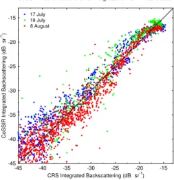
nadir and conical scan swath retrievals of ice water path and averageDme. The ice cloud retrievals are evaluated by
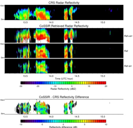
re-trieving integrated 94 GHz backscattering from CoSSIR for comparison with the Cloud Radar System (CRS) flown on the same aircraft. The rms difference in integrated backscat-tering is around 3 dB over a 30 dB range. A comparison of CoSSIR retrieved and CRS measured reflectivity shows that CoSSIR has the ability to retrieve low-resolution ice cloud profiles in the upper troposphere.
1 Introduction
to evaluate ice clouds in modern general circulation mod-els. There are several ice cloud mass remote sensing tech-niques in use from satellites, including solar reflectance (e.g., Rossow and Schiffer, 1999; King et al., 1997), nadir view-ing microwave (e.g., Ferraro et al., 2005), microwave limb sounding (e.g., Wu et al., 2006; Rydberg et al., 2009), and the CloudSat radar (Stephens et al., 2008; Austin et al., 2009). All of these approaches to sensing ice cloud mass apply to limited ranges of IWP, have limited spatial coverage, and/or have relatively low accuracy. In fact, comparisons of global ice mass datasets from these techniques (Wu et al., 2009; Eliasson et al., 2011) generally show poor agreement. Ice cloud mass can be obtained with higher accuracy from these satellite instruments using retrieval algorithms that combine instruments (e.g., Delanoe and Hogan, 2010).
High-frequency (150 GHz to 900 GHz) microwave (or submillimeter-wave) radiometry is a developing technique for remotely sensing ice cloud mass (Gasiewski, 1992; Evans and Stephens, 1995b; Evans et al., 1998, 2005; Buehler et al., 2007). Scanning submillimeter radiometry has some ad-vantages over existing techniques in that it is fundamentally more sensitive to ice particle mass (and thus potentially has the best IWP accuracy) and has good spatial coverage from low Earth orbit.
Regardless of the technique, remote sensing ice cloud mass is difficult because there are many confounding fac-tors that affect the measured radiances or backscattering. Depending on the technique, these factors include ice par-ticle shape, parpar-ticle size distribution, cloud height or temper-ature, vertical variability in the cloud, absorption by water vapor, attenuation by the cloud itself, effect of liquid cloud in and below the ice cloud, and surface emissivity or re-flectivity. Some ice cloud sensing techniques have multiple wavelengths that give independent information to solve for some of these factors, but all techniques require a priori in-formation about many of these factors. The simpler retrieval algorithms fix any factor that cannot be retrieved, for exam-ple, assuming a particular mixture of particle shapes, a fixed size distribution for each effective radius, homogeneous ice cloud, no underlying water clouds, and a specified surface albedo depending on surface type. Making these assumptions then allows forward radiative transfer modeling to be used to construct a lookup table that, for example, relates two ob-served radiances to water path and effective radius. These fixed assumptions might be fairly arbitrary or based on care-ful analysis of in situ ice cloud data and other a priori sources. More sophisticated retrieval algorithms deal with the fact that in the real atmosphere the confounding factors vary over cer-tain ranges and covary with each other.
The usual underlying framework for this approach is Bayes’ theorem and Bayesian probability concepts. In the Bayesian framework a priori information is specified with a probability density function (pdf). A Bayesian pdf specifies how likely the parameter is to have particular values. Thus, a Bayesian prior pdf should specify realistic distributions of
parameter values and their inter-relationships before the mea-surements are applied. An important example for ice clouds is that we know from in situ measurements that characteris-tic parcharacteris-ticle size is negatively correlated with temperature and positively correlated with ice water content, and both IWC and particle size are positive and have a distribution that is much closer to log-normal than normal. Bayes’ theorem says that the posterior pdf is proportional to the product of the prior pdf and the likelihood pdf, which is the conditional probability of the measurement vector given a particular at-mospheric state. In the Bayesian framework the retrieved pa-rameter, say IWP, is not a single value, but a whole posterior pdf specifying a range of likely values. It is difficult to deal with a retrieved pdf for each pixel, so usually the posterior pdf is summarized with its mean or mode and standard de-viation (or other measure of its width). In cases of multiple modes in the posterior pdf, these summarizing quantities can be quite misleading.
One special case of a Bayesian retrieval methodology that has become popular recently in ice cloud remote sensing is optimal estimation, usually in the framework developed by Rodgers (2000). Examples of retrieval algorithms that use optimal estimation include the CloudSat IWC algorithm (Austin et al., 2009) and combined radar, lidar, and infrared radiometer algorithms (Zhang and Mace, 2006; Delanoe and Hogan, 2010). The optimal estimation framework of Rodgers (2000) has also been used to explore the information con-tent of various visible and infrared wavelengths for retrieving ice clouds (Cooper et al., 2006). Optimal estimation is sim-pler and often more efficient than the fully general Bayesian framework because it assumes that the prior and likelihood pdfs are Gaussian and that the forward radiative transfer function is only moderately nonlinear. By transforming to log variables, optimal estimation can also be used easily with lognormal distributions as was done in Austin et al. (2009). Unfortunately, optimal estimation is sometimes poorly im-plemented in cloud remote sensing. The prior pdf covariance matrix is often assumed to be diagonal, ignoring the con-siderable information contained in the known correlations between variables. The prior pdf parameters are sometimes chosen somewhat arbitrarily, rather than being obtained from prior information contained in independent (e.g., in situ) datasets. Since optimal estimation uses Gauss-Newton iter-ations with the nonlinear forward model in the loop, there is a tendency to oversimplify the radiative transfer to speed the solution. Atmospheric parameters that ought to vary accord-ing to a prior pdf (because they affect the observations) are often fixed to simplify and speed the solution. For these rea-sons and because the forward function is not linear over the range of retrieval uncertainty, the retrieval errors from opti-mal estimation are usually substantially underestimated.
al., 2009). The Monte Carlo integration (MCI) method ran-domly generates atmosphere/cloud cases according to a prior probability density function and simulates instrument mea-surements for each case with a radiative transfer model to create a “retrieval database” of simulated observations and corresponding retrieval quantities. Since the cases in the re-trieval database are already distributed according to the prior pdf, Monte Carlo integration over the Bayesian posterior dis-tribution is performed by weighting the retrieved quantities in the database by the likelihood function. The likelihood function is usually assumed to be a Gaussian distribution, which is negligible unless the observation vector matches the simulated observation of the database case within the un-certainties. The standard deviation of the retrieved quanti-ties weighted by the likelihood function can give uncertainty estimates.
The algorithm of Evans et al. (2002, 2005) generated re-trieval databases having discrete ice cloud layers with cloud top altitude from a Gaussian distribution and cloud thickness from an exponential distribution. The microphysical prop-erties at the top and bottom of an ice cloud were obtained stochastically from a pdf relating temperature, IWC, and me-dian mass diameter derived from in situ cloud probe data. For each ice cloud, one of a few particle shapes was chosen randomly. Temperature and relative humidity profiles were generated stochastically using empirical orthogonal func-tions (EOFs) from statistics obtained from soundings. The Bayesian MCI method was used to retrieve IWP and median mass diameter from the observations.
Seo and Liu (2005) used EOF analysis to generalize ground-based radar reflectivity profiles and used Z-IWC re-lations to derive IWC profiles. Five different mixtures of six particle shapes and gamma distribution parameters were cho-sen stochastically. Temperature and humidity profiles were obtained by choosing from many radiosonde profiles. A database of 2.5×10⁶ cases was thus generated and used to retrieve IWP from the five AMSU-B channels (89, 150, 183.3±1,±3,±7 GHz).
Rydberg et al. (2009) generated three-dimensional (3-D) fields of ice cloud parameters using CloudSat radar data ex-panded to 3-D with a stochastic Fourier algorithm (Venema et al., 2006) and a fixed ice particle size distribution parame-terization. Temperature and humidity profiles from ECMWF were stochastically modified to introduce small-scale vari-ability. A retrieval database was generated by simulating ra-diances for the Odin-SMR limb-sounder at 501 and 544 GHz from the 3-D fields, and Bayesian MCI was used to retrieve IWC and relative humidity profiles.
The MCI method uses a database and weighting by the likelihood function to perform Bayesian retrievals. A related technique uses an a priori retrieval database to train neural networks to retrieve ice cloud parameters from brightness temperature vectors. Examples of high-frequency microwave retrievals of IWP using this neural network method include Jimenez et al. (2007) and Defer et al. (2008). Defer et al.
(2008) used a cloud resolving model with several categories of ice particles to generate a database at frequencies from 24 to 875 GHz to retrieve precipitation rate and IWP.
This paper describes a new Bayesian algorithm that re-trieves ice cloud profiles and vertically integrated parame-ters. An overview of the retrieval algorithm is given in the next section. Sections 3 and 4 describe the algorithm in de-tail. Examples of retrievals with CoSSIR data and validation with CRS reflectivities are shown in Sect. 5. Section 6 dis-cusses pros and cons of the retrieval algorithm, summarizes the results, and discusses future algorithm improvements.
2 Overview of the retrieval algorithm
The algorithm retrieves ice water content, ice particle size, and relative humidity profiles, and vertically integrated cloud parameters from microwave radiances and/or radar reflec-tivity profiles. The retrieval algorithm is tested with data from the Compact Scanning Submillimeter-wave Imaging Radiometer (CoSSIR, Evans et al., 2005) flown on the NASA ER-2 aircraft in July and August 2007 during the Tropical Composition, Cloud and Climate Coupling (TC4) experiment (Toon et al., 2010). CoSSIR measured brightness temperatures in 11 double sideband channels around 183.3, 220.0, 380.2, 640.0 and 873.6 GHz. Data are used, mostly for validation, from the nadir viewing 94 GHz Cloud Radar Sys-tem (CRS) (Li et al., 2004), also flown on the ER-2 during TC4.
with a significant contribution to the Monte Carlo integrals. The hybrid approach developed here uses MCI, but, if not enough database cases match the observation, an optimiza-tion is performed to maximize the posterior pdf. While much slower than MCI, the optimization minimizes a least squares cost function (assuming a Gaussian likelihood function) us-ing gradient information to be most efficient. There is also an option to generate the Bayesian posterior distribution us-ing the Markov chain Monte Carlo (MCMC) method, though this is only practical for testing purposes on a small number of observations. The optimization method and the generation of a large number of retrieval database cases (e.g., 106) for MCI requires using an explicit prior probability distribution rather than using CloudSat profiles individually. Another ad-vantage of using an explicit prior probability distribution is that there is some ability to extrapolate beyond the particular radar profile input.
Ice particle size distributions are defined using the parti-cle mass as expressed by the equivalent mass sphere diame-ter,De. The characteristic particle size is the IWC weighted
meanDe, and the width of the size distribution is measured
by theDedispersion:
Dme=
R
N (De) D3eDedDe
R
N (De) D3edDe
Dedisp=
1
Dme
" R
N (De) D3e(De−Dme)2dDe
R
N (De) De3dDe
#1/2 . (1) Hydrometeor layers above the freezing level can contain ice particles, specified by IWC,Dme, andDedispersion, and
liq-uid cloud droplets, specified by liqliq-uid water content (LWC),
Dme, and a fixedDedispersion. The ice particles are a
mix-ture of different shape categories, with the mixing fractions varying in the retrieval database. Below the freezing level, a simple thermodynamical melting model (with no vertical air motions) is used to calculate the melt fraction of the par-ticles (see Appendix B4). The a priori microphysics for the melting/melted particles is that of the ice particles at 273 K. The profiles of IWC,Dme, and De dispersion describe the
ice particles above the freezing level and the melting/melted particles below.
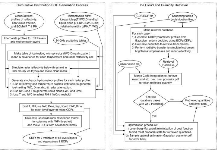
As the new ice cloud profile retrieval algorithm is de-scribed in more detail in the sections below, it will be use-ful to refer to the algorithm flowchart in Fig. 1. The profile retrieval system is divided into two separate Fortran 90 pro-grams. The first (described in Sect. 3) generates most of the a priori information and outputs a file of cumulative distri-bution functions and combined EOFs for profiles of temper-ature, relative humidity, ice and melting particle IWC,Dme,
Dedispersion, and liquid cloud LWC andDme. The second
program (described in Sect. 4) uses the CDF/EOF file infor-mation to create atmosphere and hydrometeor profiles with the desired a priori pdf, simulates the observations with ra-diative transfer, does Monte Carlo integration Bayesian re-trievals, and, when those fail, performs optimization with
gradient information to maximize the posterior pdf. Prepa-ration of the microphysical pdfs from TC4 in situ data is described in Appendix A, and generation of the scattering tables for hexagonal plate aggregates, sphere aggregates, and snowflake aggregates is discussed in Appendix B.
3 Generation of the a priori CDF/EOF file
The CDF/EOF generation program uses data from several sources to create the a priori information for the ice cloud retrieval system. The primary data source is CloudSat reflec-tivity profiles, CALIPSO lidar cloud fraction for the Cloud-Sat range bins, and the corresponding ECMWF profiles of temperature and relative humidity. The secondary sources of a priori information are parameters of several probabil-ity distributions obtained from in situ aircraft probes that describe relationships between ice cloud parameters, liquid cloud parameters, and relative humidity. Multiple profiles of IWC/LWC, Dme, and De dispersion for ice and liquid
hy-drometeors are generated for each CloudSat radar profile. Radar reflectivity does not uniquely specify ice cloud micro-physical parameters, of course, so radar reflectivity is com-bined with the ice particle microphysical statistics.
3.1 Inputs
Any number of CloudSat granules (GEOPROF, GEOPROF-LIDAR, and ECMWF-AUX files of one orbit each) may be input, and those profiles in a selected latitude-longitude box are used. All columns in the designated region or only ones deemed cloudy may be used. The altitudes of the layer in-terfaces (also called levels) for analysis and output to the CDF/EOF file are specified. The ECMWF temperature and relative humidity profiles are interpolated to the specified levels. Hydrometeors are allowed in a specified subset of the layers, and the radar reflectivity and lidar cloud fraction are averaged/interpolated to each layer. CloudSat reflectivity within three range gates of the surface elevation is not used.
Parameters of three microphysical probability distribu-tions are input. The most important one is a Gaussian distribution of T, ln (IWC), ln(Dme), and De
disper-sion for ice particles (where T is temperature). Parame-ters are input for a Gaussian distribution of T, ln (IWC), ln (LWC), ln(Dme,liq)for supercooled cloud droplets (where
LWC is the liquid water content of the droplets, and
Dme,liq is the Dme of the liquid cloud droplets).
Fi-nally, coefficients are input for the mean and standard deviation of a beta distribution of relative humidity in the presence of ice particles (T <273 K). These coeffi-cients are defined by RHmean=a+b T+c T2+dln (IWC)
and RHstddev=e+fln (IWC). Appendix A describes the
Microphysics pdfs: ice particle p(T,IWC,Dme,disp) liquid cloud p(T,IWC,LWC,Dme)
relative humidity p(RH;T,IWC) Cumulative Distribution/EOF Generation Process
94 GHz scattering tables Interpolate profiles to T/RH levels
and hydrometeor layers
Sort T, RH, ice IWC,Dme,disp, liquid LWC,Dme for each level/layer to make CDFs Calculate Gaussian rank covariance matrix
for columns with IWP>threshold and make EOFs from covariance matrix
Ice Cloud and Humidity Retrieval CDF/EOF file
Observation file
Scattering tables k-distribution files
Retrieved quantities and error bars Monte Carlo Integration to retrieve
mean and std. dev. over posterior pdf for each retrieved quantity
Too few database cases
with χ2 < threshold
no
yes
Retrieval Database
CDFs for 7 variables at all levels/layers and eigenvalues & EOFs
Make retrieval database For each case:
1) Generate T/RH/hydrometeor profiles from Gaussian random deviates using EOFs/CDFs. 2) Calculate quantities to retrieve from profiles. 3) Perform radiative transfer to simulate instrument brightness temperatures and radar reflectivity. CloudSat files:
profiles of reflectivity, lidar cloud fraction, and ECMWF T & RH
Make table of ice/melting microphysics (IWC,Dme,disp,atten) mean & covariance for each temperature and radar reflectivity cell
Simulate radar reflectivity below threshold in lidar cloudy ice layers and make cloud mask
Generate stochastic hydrometeor profiles for each radar profile: 1) Use reflectivity and temperature profiles with table to generate ice/melting IWC, Dme, disp & radar attenuation.
2) Use IWC and T to generate liquid cloud LWC and Dme. 3) Use T and IWC to adjust RH if IWC>threshold.
Optimization procedure:
1) Levenberg-Marquardt minimization of cost function to find most probable state for retrieved quantities. 2) Sample optimal estimation Gaussian posterior pdf for error bars.
Fig. 1.Flowchart of the Bayesian ice cloud profile retrieval algorithm. Abbreviations used: “T” for temperature, “RH” for relative humidity, “IWC” for ice water content, “IWP” for ice water path, “LWC” for cloud liquid water content, “Dme” for mean IWC weighted equivalent sphere diameter, “disp” forDedispersion (a measure of the size distribution width), “atten” for radar attenuation, “CDF” for cumulative
distribution function, “EOF” for empirical orthogonal function, and “pdf” for probability density function.
Tables that specify the complete scattering information for randomly oriented particles at the 94 GHz CloudSat radar frequency are used to relate the microphysical parameters to radar reflectivity. These tables specify the scattering prop-erties as a function of Dme, De dispersion, temperature,
and particle shape. There are scattering tables for the ice particles, the melting/melted ice particles, and cloud liquid droplets. See Appendix B for a description of the particle shapes used and how these scattering tables are generated.
3.2 Generation of the ice microphysics table
The radar reflectivity and ice/melting particle microphysi-cal statistics are combined by generating a two-dimensional lookup table in reflectivity and temperature (e.g., increments of 0.5 dBZ and 2.0 K, except 0.4 K in the melting zone). For each reflectivity/temperature cell of the table, the mean vec-tor and covariance matrix of ln (IWC), ln(Dme),De
disper-sion, and ln(A) (where A is the ice/melting particle radar attenuation coefficient in dB km−1) are calculated. This table is made with Monte Carlo sampling of the Gaussian
distribu-tion ofT, ln (IWC), ln(Dme),Dedispersion, random ice
par-ticle shape mixing fractions, and the appropriate scattering table (depending onT <273 K orT >273 K). The eigenval-ues and eigenvectors are calculated for the 4×4 covariance matrix in each reflectivity/temperature cell to be used later with the mean vector to stochastically simulate IWC,Dme,
Dedispersion, and radar attenuation consistent with the
re-flectivity, temperature, and the ice microphysical pdf.
3.3 Simulation of radar reflectivity below threshold
0km 15km
0km 15km
0km 15km
0km 15km
0km 15km
0km 15km
0km 15km
0km 15km
-60 -50 -40 -30 -20 -10 0 10 20
Radar Reflectivity (dBZ)
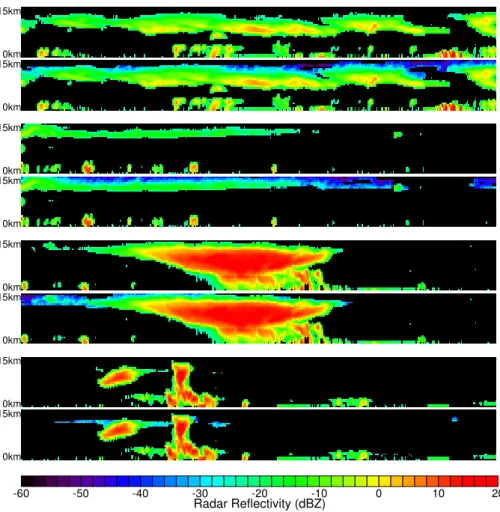
Fig. 2.An example of the stochastic simulation of radar reflectivity for lidar identified cloudy layers with CloudSat reflectivity below
−26 dBZ. For each pair of radar profiles, the top strip uses a−26 dBZ threshold without simulated reflectivity and the bottom strip includes the simulated reflectivity. There are 1600 CloudSat columns from two separate orbits over the TC4 region. The layers in this example are all 0.5 km thick.
CALIPSO lidar cloud mask. This allows the prior pdf to have lower values of IWC andDmethan would be produced from
the CloudSat reflectivity alone. An example of the radar re-flectivity profiles with and without the simulated rere-flectivity is shown in Fig. 2.
To prevent discontinuity in the CDFs, layers identified as clear are set to very small, random reflectivity values that are correlated in the vertical. The correlation matrix for generat-ing these fictitious reflectivity values is calculated from the radar reflectivities above the noise threshold. The mean and standard deviation of these stochastic reflectivities for clear layers are−80 dBZ and 1 dBZ, respectively.
3.4 Generation of stochastic hydrometeor profiles
The lookup table is used to generate several stochastic hy-drometeor parameter profiles for each CloudSat reflectivity profile. First, the CloudSat reflectivity profiles are corrected for molecular attenuation with the absorption profile pro-vided in the GEOPROF file (Marchand et al., 2008). For
each hydrometeor profile, four independent stochastic pro-files of zero mean/unit variance Gaussian deviates are gen-erated having the same vertical correlations as the radar re-flectivity. These Gaussian profiles are used with the reflectiv-ity/temperature lookup table to stochastically generate IWC,
Dme, De dispersion, and attenuation (dB km−1) that agree
ice particles (i.e., rain) and not for cloud droplets, bound-ary layer clouds or shallow convection. In deep convection, multiple scattering increases CloudSat reflectivity above the single scattering values assumed here. Battaglia et al. (2011) estimated that, in tropical deep convective cores, multiple scattering becomes important (>3 dBZ) below about 9 km altitude. Since correcting for multiple scattering accurately is very difficult, we simply note that the effect is to over-estimate the (single scattering) 94 GHz reflectivity when the reflectivity is high (>10 dBZ), thereby widening the a priori IWC andDmedistributions.
Liquid cloud LWC andDmefor layers above the melting
level are generated stochastically using the Gaussian distri-bution in T, ln (IWC), ln (LWC), ln(Dme,liq)with vertical
correlations according to the radar correlation matrix, but with some thresholds applied. There is no supercooled liq-uid cloud colder than a threshold temperature (e.g., 240 K to be consistent with the data used to generate the distribution). If the generated liquid cloud LWC is below 0.01 g m−3, then it is set to zero, since the Bergeron-Findeisen process would tend to eliminate small LWC in the presence of ice crys-tals. The cloud liquid water content andDmebelow the
melt-ing level are linearly interpolated between that of the lowest supercooled layer and the approximate lifting condensation level.
The relative humidity profile from the CloudSat ECMWF file is adjusted in the presence of significant ice water con-tent using the coefficients of the beta distribution mean and standard deviation. The IWC has to be above a threshold (now 0.001 g m−3) before the relative humidity is adjusted.
Instead of choosing a beta deviate randomly, the “probabil-ity” (0 to 1) of the ECMWF relative humidity in its cumula-tive distribution is translated to the beta deviate. Thus, a low ECMWF humidity will result in a relative humidity from the low end of the beta distribution that depends on temperature and IWC. This procedure also results in the relative humid-ity having reasonable vertical correlations. If there is nonzero cloud liquid water content in a layer, then the relative humid-ity is set to 100 %.
3.5 Calculating CDFs and EOFs
Cumulative distribution functions,Di(xi), are made by
sort-ing (over all the stochastic hydrometeor profiles generated from the radar profiles) the temperature and relative humidity for each profile level and the hydrometeor parameters (IWC,
Dme,Dedispersion and liquid cloud LWC andDme) for each
hydrometeor layer. At this point, the seven parameters for each level/layer in the profiles (generically denoted by xi)
are represented by the probability,pi, or rank in the CDFs,
i.e.,pi=Di(xi), wherei specifies both the parameter and
the profile level/layer.
A type of rank correlation matrix is used to generate the EOFs with the desired correlations. Thus, the joint prob-ability distribution between two variables (e.g., IWC and
Dme in two layers) is represented by a single number, i.e.,
the correlation. To make the correlations more representative of the important relationships for ice cloud retrievals, only those profiles with IWP above a specified threshold (e.g., 10 g m−2) are used for the correlations. This is done by hav-ing a second set of CDFs, Di,IWP>(xi), made from those
profiles with IWP above the threshold. The ranks or prob-abilities representing the profiles are converted to Gaussian deviates using
ξi =8−1Di,IWP> (xi), (2)
where8 (ξ ) is the cumulative distribution function of the standard normal distribution. Gaussian distributions work best with EOFs, because linear combinations of indepen-dent Gaussian deviates remain Gaussian. The covariance ma-trix for the EOFs is calculated from these Gaussian deviates. Since the Gaussian deviatesξihave zero mean and unit
vari-ance, the covariance matrix is also the correlation matrix:
Cij =
1
Nprof
Nprof
X
k=1
ξi(k)ξj(k), (3)
where the sum is over theNprofstochastic profiles with IWP
above the threshold for the correlation matrix. The eigenvec-tors of the correlation matrix,Cij, are the EOFs.
The output CDF/EOF file contains the heights of the pro-file levels and hydrometeor layers; the CDFs of temperature, relative humidity, IWC,Dme,Dedispersion, and liquid cloud
LWC andDmefor each level or layer; and the Gaussian EOF
eigenvalues and eigenvectors.
3.6 Example CDFs and rank correlation matrix
region (about 5 to 15 km). The a priori IWC profiles have a tremendous range from effectively clear (<10−5g m−3) to about 10 g m−3. Similarly,Dmeranges from below 15 µm
to above 1500 µm, though the maximumDme generally
de-creases with height. The 95th percentile of IWC shows that the highest IWCs are deep, ranging from the surface to about 14 km. The highest layer cloud fraction (up to 45 % for 0.5 km layers) is in the anvil region from 10 to 14 km. In-cluding the correlations between layers, the resulting cloud fraction is about 89 %. The peak layer liquid cloud fraction is about 11 % near the melting level.
Figure 6 shows the correlation matrix used to make the EOFs with each part of the matrix labeled by the parame-ters. Nearby layers of temperature, relative humidity, IWC, andDme are highly correlated. IWC and Dme of the same
layer have a reasonably high rank correlation. The fairly high correlation between relative humidity and IWC can be seen. Although there seems to be a lot of information in the cor-relation matrix, and hence the EOFs, it should be noted that there is only one number to represent the relationship be-tween any two variables, which is a tiny fraction of the in-formation contained in a joint probability distribution. It is, however, the same amount of information contained in the multi-variate Gaussian distribution assumed in the optimal estimation method.
4 Ice cloud/humidity profile retrieval process
The inputs to the retrieval program are (1) the CDF/EOF file of a priori information, (2) a file of observation vectors (with measurement uncertainties and viewing directions), (3) a re-trieval database file, and (4) many parameters and files that define the characteristics of the retrievals and measurements and provide data for the radiative transfer calculations. The retrieval program is run in one of two modes: (1) gener-ate and output a retrieval database, or (2) read a retrieval database and perform retrievals. For each database “case”, an atmosphere/cloud profile is generated with the desired a pri-ori information from the CDF/EOF file information, and then the radiative transfer is done to simulate the observations.
4.1 Atmosphere profile generation
The atmosphere/cloud profile generation process begins with generating a vector of independent, standard Gaussian ran-dom deviates (ξ), most of which are used to drive the EOFs. The number of EOFs used is user specified, and may be chosen, for example, to include 99 % of the variance. The Gaussian deviates are multiplied by the square root of the eigenvalues to make the random EOF coefficients, which are then multiplied by the eigenvector matrix to give a long vector of correlated Gaussian distributed elements. Gaus-sian random deviates are used because the GausGaus-sian distri-bution shape is preserved upon the linear EOF
transforma-200 220 240 260 280 300
Temperature (K) 0
5 10 15 20 25
Height
(km)
A Priori Temperature Profiles
100% 95% 75% 50% 25% 5% 0%
0.0 0.1 0.2 0.3 0.4 0.5 0.6 0.7 0.8 0.9 1.0 Relative Humidity 0
5 10 15 20 25
Height
(km)
A Priori Relative Humidity Profiles
100% 95% 75% 50% 25% 5% 0%
Fig. 3.Profiles of temperature and relative humidity from seven per-centiles in the a priori cumulative distribution functions.
tion. These Gaussian distributed elements are converted to probabilities,pi, with uniform distributions between 0 and 1
using the standard normal cumulative distribution function, i.e., pi=8 (ξi). These correlated “probabilities” are then
used to index into the temperature, relative humidity, and hydrometeor CDFs to produce the correlated profiles, i.e.,
xi=D−i 1(pi).
The relative humidities are converted to water vapor mix-ing ratioq, since that is what the radiative transfer routines require. This conversion requires the pressure profile, which is derived from the temperature profile using the hypsometric equation. If the relative humidity profile is to be a retrieved quantity, then desired levels are stored in the retrieval vector. The hydrometeor profiles are IWC,Dme, andDe
disper-sion for the ice/melted particles, and the LWC andDmefor
cloud liquid droplets. If the layer temperature is below the melting temperature, the IWC andDmeare used for the ice
particle component, and, if the temperature is above the melt-ing temperature, the IWC andDme are used for the
melt-ing/melted particle component. To preserve differentiability, this temperature threshold is implemented with a smooth ex-ponential that quickly varies between 0 and 1. The liquid cloud droplet LWC andDme are applied to the third
com-ponent, and theDe dispersion is set to 0.3. In the radiative
transfer, each hydrometeor component (ice, melting, liquid droplets) is associated with its own set of scattering tables (one for each frequency).
Another set of (Nlayer,shape+ 1) Nshape Gaussian deviates
(fromξ) is used to control the ice particle shape mixing frac-tion of the Nshape possible shapes in the scattering tables
atNlayer,shape+ 1 heights in the hydrometeor profiles.
Test-ing finds that linear interpolation over the whole ice region
(Nlayer,shape= 1) gives an adequate number of degrees of
10-6 10-5 10-4 10-3 10-2 10-1 100 101
Ice Water Content (g m-3)
0 2 4 6 8 10 12 14
Height
(km)
A Priori IWC Profiles
100% 95% 75% 50% 25% 5% 0%
10 20 50 100 200 500 1000 2000
Dme( m)
0 2 4 6 8 10 12 14
Height
(km)
A Priori DmeProfiles
100% 95% 75% 50% 25% 5% 0%
0.0 0.1 0.2 0.3 0.4 0.5 0.6 0.7 0.8 0.9 1.0
DeDispersion
0 2 4 6 8 10 12 14
Height
(km)
A Priori DeDispersion Profiles
100% 95% 75% 50% 25% 5% 0%
Fig. 4.Profiles of IWC,Dme, andDedispersion from seven percentiles in the a priori cumulative distribution functions. Below the freezing
level, the profiles are applied to the melting/melted particles instead of the ice particles.
0.0 0.5 1.0 1.5 2.0 2.5 3.0
Liquid Water Content (g m-3)
0 2 4 6 8 10 12 14
Height
(km)
A Priori cloud LWC Profiles
100% 95% 75% 50% 25% 5% 0%
0 10 20 30 40 50 60
Dme( m)
0 2 4 6 8 10 12 14
Height
(km)
A Priori Liquid Cloud DmeProfiles
100% 95% 75% 50% 25% 5% 0%
Fig. 5.Profiles of liquid cloud LWC and Dme from seven
per-centiles in the a priori cumulative distribution functions.
height toNshapefractions at each hydrometeor layer. These
fractions are then adjusted according to the layer Dme so
that the mixing fraction is set to zero for particle shapes for which theDme is outside the range in the scattering tables
(and the shape mixing fractions sum to 1). Thus, the parti-cle shape mixing fractions are not controlled by the a priori CDF/EOF process, but are considered completely unknown prior to the observations. There is, however, prior informa-tion about the particle shape in that only certain shapes are available at a givenDme; for example, hail is only available
forDme>398 µm.
Four vertically integrated quantities, IWP, average Dme,
median IWP height (Zmed), and melted liquid water path
(LWP), are calculated from the IWC andDmeprofiles and
stored in the retrieval vector. The IWC weighted shape mix-ing fractions and cloud droplet LWP are also stored in the
Temp RH IWC Dme Dedisp LWCcld Dme,cld
Layer/Variable
Temp RH IWC
Dme
Dedisp
LWCcld
Dme,cld
Layer/V
ariable
Gaussian Rank Correlation Matrix
-1 -0.5 0 0.5 1
Fig. 6.The Gaussian correlation matrix used to make the EOFs. Blue is a correlation of−1, white a correlation of 0, and red a cor-relation of 1. Each element of the matrix represents a pair of param-eters and layers, with increasing height of the levels/layers within each parameter block. TheT and RH levels from the surface up are shown as dots in Fig. 3, while the hydrometeor layer centers are shown as dots in Fig. 4.
retrieval vector. If desired, the IWC and Dme profiles at a
specified resolution are stored in the retrieval vector.
4.2 Radiative transfer
though there could be options for other radiative transfer models in the future. SHDOMPPDA was chosen because an adjoint, which is needed for the optimization, was already de-veloped. It can perform unpolarized solar and thermal emis-sion radiative transfer for randomly oriented particles, and is flexible in the trade-off between accuracy and computa-tional efficiency. The radiative transfer module also supports calculating radar reflectivity profiles and vertically integrated backscattering, which includes attenuation by gases and par-ticles, but not multiple scattering. A k-distribution system is used to calculate molecular absorption given the profiles of temperature, pressure, water vapor and ozone mixing ra-tio. The script for generating the k-distribution table for each channel with LBLRTM (Clough et al., 2005) includes the spectral response of the channel. For CoSSIR and CRS a fourth-order Butterworth filter response is assumed for the bandpasses, and, of course, only one “k” is needed for these nearly monochromatic channels. The surface reflection is simply specified with the mean and standard deviation of the stochastically varied Lambertian emissivity, which is either completely correlated or uncorrelated between channels. A few elements of the Gaussian deviate vectorξ are used to vary the surface emissivity.
The single scattering properties are input with a scatter-ing table for each channel. The scatterscatter-ing tables have the ex-tinction, single scattering albedo, and Legendre series of the phase function tabulated as a function ofDme,De
disper-sion, particle shape, and temperature. The temperature de-pendence is needed in the microwave, especially for liquid water, but also for the weak absorption of ice. The range of
Dmetabulated varies with particle shape. The optical
proper-ties are interpolated in ln(Dme),Dedispersion, and
temper-ature using successive cubic splines. The gradients of cubic spline interpolation are continuous, which is important for the gradient-based optimization calculation. A trilinear inter-polation option is also available if optimization is not go-ing to be used. Interpolation is performed on log extinction, single scattering albedo, and the Legendre coefficients.
4.3 MCI and optimization retrieval methods
The primary and most efficient solution method used in the ice cloud profile Bayesian retrieval algorithm is Monte Carlo integration (MCI) (e.g., Evans et al., 2002). Random atmo-spheric/cloud profiles distributed according to the a priori pdf are generated as described above. The retrieval database con-tains the desired retrieved quantities (e.g., IWP, meanDme,
Zmedand perhaps IWC/Dmeand relative humidity profiles)
and the associated simulated observations (e.g., brightness temperature for each channel and a radar reflectivity pro-file) for one or more viewing angles. Specified simulated channels in the retrieval database may be treated as retrieved parameters, so that one instrument may be used to retrieve observables of another for comparison.
The MCI algorithm calculates the conditional pdf (or like-lihood function) in Bayes’ theorem, which is assumed to be an uncorrelated Gaussian distribution in the difference be-tween the simulated and measured observations. Since the database cases are distributed according to the a priori pdf, the conditional pdf is the same as the posterior pdf:
ppost ∝exp
−1
2χ
2
χ2 =
Nchan
X
j=1
yj(sim)−yj(obs)
2
σj2 (4)
whereyj(sim)andyj(obs) are the simulated and measured ob-servations in channelj with a combined measurement and forward modeling uncertainty ofσj. The retrieved quantities
(e.g., IWP) are the posterior pdf weighted means,
Wret=
P
i
Wiexp
−12χi2
P
i
exp−12χi2
, (5)
and the retrieved uncertainty is the weighted standard devi-ation. There is an option to perform the integration in log space for the cloud parameters (IWC andDme). The
proba-bility of an ice cloud is retrieved from the ratio of the sum of the posterior probability of cases using
pcloud =
P
i
exp−12χi2 for IWPi >IWPclear
P
i
exp−12χi2
. (6)
If a particular measurement is flagged as bad, then the corre-spondingσjis multiplied by 1000 to effectively ignore it. For
a cross-track scanning instrument, there are multiple viewing angles stored in the retrieval database and the simulated ob-servations are interpolated to the actual observation viewing angle. If the number of database cases with anχ2less than a user-specified threshold is below a specified number, then the Monte Carlo integration is said to have failed, and the slower optimization process is begun for that observation vector.
The control vector for the optimization is the indepen-dent Gaussian deviates (ξ), not the geophysical variables derived from them in making the atmosphere/cloud pro-files. This is natural given the connection to the Monte Carlo integration retrieval method, and means that the atmo-sphere/cloud/surface a priori information is contained in the function that relates the geophysical variables (x) to the con-trol vector, i.e.,x=G(ξ). In data assimilation this approach is called control variable transformation (Bannister, 2008). If the radiative transfer function isFj(x), the posterior pdf is
then maximized by minimizing the cost function (J):
J =
Ndim
X
i=1
ξi2+
Nchan
X
j=1
yj(obs)−Fj[G(ξ)]
2
The first term is the formal background or a priori from the independent Gaussian distribution of the state vector ele-mentsξi, while the second term is the observationalχ2. This
assumes that the observational uncertainties combined with the radiative transfer errors are Gaussian and independent in each channel. Internal to the retrieval program, the database stores the control vectors (ξ), and the optimization is initial-ized with theξof the case having the minimumχ2.
The advantage of having the cost function in the least squares form is that the robust and efficient Levenberg-Marquardt minimization method may be used. The quadratic form of the formal background term in the cost func-tion also means that the optimal estimafunc-tion framework of Rodgers (2000) may be applied even though the real a pri-ori distribution (contained inG(ξ)) is highly non-Gaussian. The Levenberg-Marquardt formulation described in Rodgers (2000) (Sect. 5.7) is implemented. This requires the Jacobian of the forward functionF[G(ξ)], or theKmatrix in the no-tation of Rodgers. TheKmatrix is calculated using the ad-joint of the radiative transfer for each channel (Fj (x)) and
the adjoint of the a priori functionG(ξ)that calculates the geophysical variables from the control vector.
The optimization process to find the retrieval solution does not provide the uncertainties of the retrieval, as the Monte Carlo integration method does. Therefore, the local Gaus-sian approximation used in the optimal estimation frame-work (Rodgers, 2000) is implemented to distribute points around the solution (ξmin) in control vector space to
char-acterize the retrieval uncertainty. The local Gaussian ap-proximation method computes the optimal estimation error covariance matrix. This assumes that the forward function
F[G(ξ)]is only moderately non-linear, so that the lineariza-tion and Gaussian distribulineariza-tion assumplineariza-tions are valid. The op-timal estimation posterior error covariance matrix is
S=S−a1+KTS−y1K
−1
(8) whereKis the linearization matrix ofF[G(ξ)],Sythe
ob-servational error covariance matrix, assumed here to be di-agonal with elementsσj2, andSais the a priori error
covari-ance matrix, which here is the covaricovari-ance ofξand is thus the identity matrix. The Cholesky decomposition ofSis used to generate random points with a correlated Gaussian distribu-tion aroundξmin. Of course, we are not interested in the error
characterization in control vector space, so the random points inξ are transformed to the atmosphere/cloud profiles and a Monte Carlo integration is done over the retrieval quantities. Since this step does not involve radiative transfer, a large number of Monte Carlo samples (e.g., 1000) can be used in the integration.
4.4 Markov chain Monte Carlo solution method
The Markov chain Monte Carlo (MCMC) technique is devel-oped as an optional solution method to check the accuracy of
the optimization/local Gaussian approximation method. The MCMC has been applied in atmospheric remote sensing for several low-dimensional retrieval problems (e.g., Tamminen and Kyrola, 2001; Posselt et al., 2008). Here a more advanced “stochastic approximation adaptive” MCMC approach, ba-sically Algorithm 4 in Andrieu and Thoms (2002), is used. The MCMC method creates a Markov chain of control vec-tors ξi that are distributed according to the Bayesian
pos-terior distribution, which here is exp(−J /2). The Markov chain is started at the optimization end point (ξmin), so
it-erations are not wasted finding the high probability region of the control vector space. The basic Metropolis algorithm step of MCMC is to calculate a trial control vector point in the Markov chain (ξtrial) from the current point (ξi) using a
symmetric “proposal distribution” centered onξi. The cost
function,J (ξtrial), at the trial point is computed and
com-pared to the current point cost function,J (ξi), by defining
an acceptance ratio,α:
α=MIN
1, exp
−1
2 [J (ξtrial)−J (ξi)]
. (9)
The trial point is accepted, ξi+1=ξtrial, if a uniform
ran-dom number is less than the acceptance ratio, and otherwise
ξi+1=ξi (the current point is reused). In adaptive MCMC
the proposal distribution is updated according to the history of the Markov chain, i.e., theξi vectors. As is usually done,
here the proposal distribution is taken to be a multivariate Gaussian distribution with covariance matrixλi6i, so that
ξtrialis sampled fromN (ξi, λi6i). The “stochastic
approx-imation” part of the adaptive MCMC algorithm is that the mean (µi) and covariance matrix (6i) of the control vectors
are continuously updated according to a relaxation parameter
γ that smoothly decreases to zero:
µi+1=µi +γi+1(ξi+1−µi)
6i+1=6i +γi+1
h
(ξi+1−µi) (ξi+1−µi)T −6i
i .(10) Since this updating formula is not guaranteed to keep the co-variance matrix positive definite and the Cholesky decompo-sition of6is needed to generate the random trial points, ac-tually the Cholesky decomposition is updated. The Cholesky updating formula in Sect. 5.1.1 of Andrieu and Thoms (2002) is incorrect, so an algorithm that is first-order inγ was de-rived from the Cholesky decomposition algorithm. The pro-posal distribution covariance scaling parameterλiis also
up-dated with a stochastic approximation formula:
λi+1 =λi expγi+1(α−α∗), (11)
so that the mean acceptance ratio converges to the target
α∗= 0.234. Here the relaxation parameterγ is decreased
ac-cording to a power law in the iteration numberi, specified by the power and final relaxation parameter value (thoughγ
13.5 14.0 14.5 15.0 140
160 180 200 220 240 260 280
Brightness
T
emperature
(K)
CoSSIR nadir Tband retrieved cloud probability and IWP (19 July 2007)
Tb,874
Tb,640V
Tb,220
Tb,183 1.0
13.5 14.0 14.5 15.0
0.0 0.2 0.4 0.6 0.8 1.0
Ice
Cloud
Probability
13.5 14.0 14.5 15.0
UTC Time (hour) 3
10 30 100 300 100 300 1000 3000 10000
Ice
W
ater
Path
(g
m
-2)
..
...
.
.
.
...
.
.
..
.
.
.
...
.
...
.
..
.
..
.
.
.
..
.
..
...
.
.
..
.
...
.
.
.
.
.
..
..
....
...
..
...
.
...
...
...
...
...
.
...
...
.
...
.
.
.
...
...
.
.
.
.
..
.
....
..
...
...
....
...
...
...
..
.
.
.
.
...
.
.
.
...
...
.
...
.
...
.
..
.
.
.
.
..
..
...
.
....
.
..
...
..
.
.
.
..
..
..
.
....
...
...
..
.
....
....
...
...
...
...
...
...
...
.
.
.
.
.
.
...
...
....
..
...
.
...
.
.
.
...
.
....
.
...
.
..
..
.
....
.
..
.
.
.
...
..
.
.
.
.
.
.
...
.
.
.
.
...
.
..
.
..
.
.
Fig. 7. CoSSIR brightness temperatures for four channels (top panel). Retrieved probability of ice cloud (middle panel). A dotted line at 0.95 probability is shown. Retrieved ice water path (bottom panel).
Carlo integration over the posterior distribution to calculate the mean parameters for the retrievals and the standard de-viations for the errors. In this application the number of it-erations must be very large (>105) so that the MCMC so-lution method is impractical for use on whole datasets. The MCMC method is, however, useful for comparison with the other solution methods for a small number of pixels.
5 Example retrieval results
During TC4, CoSSIR measured brightness temperatures in channels around 183.3, 220.0, 380.2, 640.0 and 873.6 GHz, all with matched beamwidths of about 4◦. The CoSSIR scanning pattern consisted of three parts during each 10 s scan: forward and aft conical scans and two quick cross-track scans through nadir. The beam dwell (integration) time is 100 ms for the conical scans, but only 10 ms for nadir view, which results in about three times the receiver noise for nadir pixels. Due to hardware problems during the cam-paign, CoSSIR data from ice clouds are available only for the 17 July, 19 July, and 8 August flights. The Cloud Radar System (CRS) is a Doppler, polarimetric radar, though only the reflectivity profiles from the NASA Earth Science Project Office (ESPO) archive are used here. The CRS antenna beamwidth is 0.6◦by 0.8◦and views nadir. The CRS sensitiv-ity is−29 dBZe at 10 km range with 150 m range resolution and 1 s averaging.
13.5 14.0 14.5 15.0
3 10 30 100 300 100 300 1000 3000 10000 30000
Ice
W
ater
Path
(g
m
-2)
CoSSIR Retrieved Nadir IWP, Dme, and Zmed(19 July 2007)
. ...
....
.
..
...
...
...
.
...
...
...
...
...
..
...
...
.
...
...
..
.
..
.
....
...
...
...
...
...
...
..
.
..
.
...
.
...
.
.
....
...
...
...
....
...
...
...
...
...
...
...
...
...
...
.
...
... .
13.5 14.0 14.5 15.0
50 100 200 500 1000
Dme
(
m)
. ...
..
.
...
.
...
...
..
....
..
...
...
....
.
.
.
...
.
.
...
....
..
.
...
...
.
...
...
..
...
.
..
...
.
.
...
.
...
...
...
..
...
.
.
...
...
.
...
.
...
.
...
..
...
.
...
...
...
...
.
....
...
....
...
.
...
.
.
...
.
..
....
...
....
..
.
..
....
...
....
...
...
....
...
..
...
.
...
...
.
... .
13.5 14.0 14.5 15.0
UTC Time (hour) 4
5 6 7 8 9 10 11 12 13 14
Median
IWP
Height
(km)
. .
....
...
..
.
...
..
...
....
.
.
...
..
...
.
...
....
.
.
..
.
.
...
...
...
...
..
...
.
.
....
.
....
.
...
....
.
.
...
..
...
...
.
...
.
..
...
..
...
.
.
...
...
.
...
.
...
.
...
...
.
...
...
...
...
.
..
...
...
....
.
..
..
.
...
...
.
...
.
...
....
.
...
.
.
..
..
.
.
...
.
...
...
.
..
...
...
...
...
.
.
...
..
..
...
...
.
..
.
...
..
..
.
.
...
.
..
.
.
..
.
..
...
...
.
....
..
...
.
..
...
.
.
...
...
... .
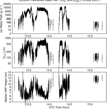
Fig. 8.CoSSIR retrieved ice water path (top panel),Dme(middle
panel), and median IWP height (bottom panel) for cloudy nadir pix-els of the 19 July flight. 1-σerror bars are shown for each retrieved quantity.
Retrievals are performed mostly with CoSSIR nadir viewing data obtained 19 July from 9 CoSSIR channels (183.3±1.0, 3.0, 6.6, 220, 380.2±1.8, 3.3, 6.2, 640 V, and 874 GHz). The CoSSIR uncertainties (σs), obtained from calibration target fluctuation statistics, are 1.60, 1.62, 1.59, 1.59, 2.00, 2.45, 2.36, 2.38, 4.03 K for the 9 channels used on 19 July. Retrievals from CoSSIR brightness temperatures are also done for the same 9 channels on 17 July and for 6 chan-nels on 8 August (without the 380 GHz chanchan-nels because the 380 GHz receiver failed). The CoSSIR uncertainties (σs) are somewhat different for these two other flights. The CoSSIR channels are used to directly retrieve 94 GHz radar reflectiv-ity profiles. The profile retrieval algorithm is also used to op-erate on CRS reflectivity profiles alone or with CoSSIR nadir data. When CRS radar reflectivity is input to the retrieval, it is averaged from 75 m resolution to 500 m (20 layers from 5 to 15 km) and has a multiplicative uncertainty of 0.4 (an estimated calibration uncertainty of about 1.5 dB). The CRS radar additive uncertainty is calculated from a clear region, and ranges from about 0.0028 mm6m−3 (−25.5 dBZ) near the surface to about 0.0003 mm6m−3(−35 dBZ) at 15 km.
The retrievals are performed using the CDF/EOF file, for which results are shown in Sect. 3. The first 146 EOFs of the total of 246, which have 99 % of the variance, are used. Monte Carlo integration retrievals are done with a retrieval database of 106cases. At least 25 cases with a reduced χ2