Leading Edge Device Aerodynamic Optimization

(1)

Marius Gabriel COJOCARU*

,1

, Mihai Leonida NICULESCU

1

, Dumitru PEPELEA

1

*Corresponding author

1

INCAS - National Institute for Aerospace Research

“

Elie Carafoli

”

,

Flow Physics Department, Numerical Simulation Unit

B-dul Iuliu Maniu 220, Bucharest 061126, Romania

cojocaru.gabriel@incas.ro*, niculescu.mihai@incas.ro, pepelea.dumitru@incas.ro

DOI: 10.13111/2066-8201.2015.7.4.7

Received: 05 October 2015 / Accepted: 02 November 2015

The 36th“Caius Iacob” Conference on Fluid Mechanics and its Technical Applications 29 - 30 October, 2015, Bucharest, Romania, (held at INCAS, B-dul Iuliu Maniu 220, sector 6)

Section 2. Numerical Analysis

Abstract: Leading edge devices are conventionally used as aerodynamic devices that enhance performances during landing and in some cases during takeoff. The need to increase the efficiency of the aircrafts has brought the idea of maintaining as much as possible a laminar flow over the wings. This is possible only when the leading edge of the wings is free from contamination, therefore using the leading edge devices with the additional role of shielding during takeoff. Such a device based on the Krueger flap design is aerodynamically analyzed and optimized. The optimization comprises three steps: first, the positioning of the flap such that the shielding criterion is kept, second, the analysis of the flap size and third, the optimization of the flap shape. The first step is subject of a gradient based optimization process of the position described by two parameters, the position along the line and the deflection angle. For the third step the Adjoint method is used to gain insight on the shape of the Krueger flap that will extend the most the stall limit. All these steps have been numerically performed using Ansys Fluent and the results are presented for the optimized shape in comparison with the baseline configuration.

Key Words: high lift devices, optimization, laminar wing.

1. INTRODUCTION



(2)

shielding. Such a leading edge device is the Krueger flap, which has been proven on Boeing 727 in-board wing section and Boeing 747. The advantage of the Krueger flap is two-fold. Firstly unlike the slat it does not introduce a gap or a step on the upper side of the airfoil, and secondly it shields the airfoils leading edge from contamination. In this work we present a method for optimizing such a leading edge device in the shape of a Krueger flap that is able to recover the aerodynamic performance of a slat. To simplify our presentation we will consider an outboard section of the wing in order to eliminate the need to consider the trailing edge flap and its influence on the flow. Also for the sake of brevity we will consider only a 2D analysis of the flow. The optimization process is numerically performed in Ansys Fluent and Ansys Workbench environments. The process consists of three steps: the determination of the Krueger flap size, the optimization of the Krueger flap position and the optimization of the Krueger flap shape.

2. GENERAL CONSIDERATIONS REGARDING NUMERICAL

MODELLING

Ansys - Fluent is a CFD software that has a very broad range of applications. The code uses the finite volume approach to discretize the Navier-Stokes equations (and their approximations Reynolds-Averaged Navier-Stokes, Large Eddy Simulation, etc.) and a wide array of related equations such as energy conservation, passive scalar transport equations, heat transfer, chemical reactions, noise propagation, adjoint equations, etc. to solve the fluid flow and fluid flow related problems. This flexibility allows us to use Fluent to solve the compressible and incompressible fluid flow around a wing with deployed high lift devices. The assumptions made in the current flow computations are:

• The medium is considered to be a continuum.

• The flow is turbulent over the full domain, the reference Reynolds number based on airfoil chord is of the order of 10 Million.

• The equation of state is that of an ideal gas.

• The flow is compressible, although the far-field Mach number is 0.2, the flow can be locally accelerated in the compressible regime (Fig. 2).

• The equations are cast in the conservative form, and the solver is “density based”, Roe method is used for flux discretization and second order accuracy is achieved by reconstructing the conservative variables.

• The solution sought corresponds to a steady state.

Since we assume the flow to be governed by a compressible ideal gas at a fully turbulent regime we can use the RANS equations. The RANS approach is based on the k-ω STT turbulence model that uses the Boussinesq hypothesis. This model was proposed by Menter and combines the advantages of traditional Low-Reynolds k-ω models near the wall with the classical k-ε models far from the walls, the two models are combined through blending functions. This model has proved to be useful in computing compressible external flows and accurately predicting boundary layer separation and aerodynamic forces/moments for largely separated steady flows. The equations are solved in the implicit approach and solution acceleration is made using the Algebraic Multi-Grid method.

Regarding the Adjoint solver available within Fluent, several remarks have to be made:

(3)

flow solver.

• The adjoint solver calculates the derivative of a single engineering observation (force, moment, pressure drop, mass flow, heat flux, etc.) with respect to a very large number of input parameters.

• The flow state is for a steady incompressible single-phase flow that is either laminar or turbulent.

• For turbulent flows a frozen turbulence assumption is made, in which the effect of changes to the state of the turbulence is not taken into account when computing sensitivities.

• For turbulent flows standard wall functions are employed on all walls.

• The adjoint solver uses methods that are first order accurate in space by default, but second order accurate methods can be also used.

Therefore when using the adjoint solver a second grid with a y+ ~ 30 has been constructed that was more appropriate for the use of standard wall functions in conjunction with the k-ε turbulence model. Also the flow solution used in the adjoint solver is computed in the incompressible assumption. In these computations the observable was the gliding ratio, whose sensitivity was computed with reference to the shape change.

The typical use of the adjoint solver involves the following steps:

1. Compute a conventional flow solution with the above assumptions. 2. Load the adjoint solver.

3. Specify the observable of interest and set the adjoint solver controls, monitors and convergence criteria.

4. Initialize the adjoint solution and iterate to convergence.

3. OPTIMIZATION PROCESS

As stated previously the optimization consists of three major steps. In the following we will discuss in detail each individual step.

3.1 Krueger flap size

The size of the Krueger flap has to be addressed by taking into account the maximum extent of the stowed flap and the position of the wings torsion box and the space allocation in front of it. Considering that the latter is fixed and that the forward extent of the stowed Krueger cannot go below 1% of the chord and that the Krueger’s upper surface must coincide with the clean airfoil lower side, we are left to optimize the Krueger size by analyzing the influence of the Krueger’s trailing edge on its performance.

When using the 1% of the stowed Krueger (maximum Krueger size) we would expect to have a higher lift when compared to 1.5% and 2% (minimum Krueger size considered), since the area is smaller a lower lift is expected. When comparing the flow solution obtained with the k-ω STT turbulence model on a grid that has a y+ ~ 1 for a Mach of 0.2 and a AoA of 5°

we can see a detached flow at the Krueger’s Trailing Edge (TE) for the 1% case (Fig. 1) and no such flow for the 2% case (Fig. 2). This detached flow can have negative impact on the

airfoil’s upper surface thus degrading the gliding ratio performance. This is due to the fact that at 1% from the Leading Edge (LE) of the airfoil the lower surface curvature is very pronounced when compared to the 2%.

The 1.5% position shows similar trends to the 1% case. Therefore in the following we

(4)

Fig. 1 –1% forward extent of the stowed Krueger flap.

Fig. 2 – 2% forward extent of the stowed Krueger flap.

3.2 Krueger flap position

The Krueger flap position is defined by a set of 3 parameters: gap, overlap and deflection angle. Considering that the flap has to be positioned on a fixed line, called the shielding line, the three parameters can be deduced from just two others parameters (DoF in Fig. 3). DoF 1 is a simple translation on the shielding line and DoF 2 is a rotation around a point that is the

intersection of the Krueger’s TE and the shielding line. DoF 1 is responsible for the gap and overlap while DoF 2 is responsible for the deflection angle.

Ansys Workbench is an enviroment capable of integrating the parametric geometrical modeling, automatic meshing, automatic solution procedure with an optimization algorithm. Thus we have constructed a parametric geometry from the two parameters (DoF 1 & 2) and then we setup an automatic mesh and solution procedure. The meshes (Fig. 4) are automatically computed with the same characteristics (number of points on the surface, boundary layer inflation factor, number of layers and first layer height) and passed to automatically to the Fluent solver who returns the lift and drag. The gliding ratio (ratio of lift over drag) is then used by the Ansys Workbench Direct Optimization tool to search for an optimum. This solution is performed in a gradient based optimization manner. On the other hand if instead of the gliding ratio the lift is imposed to be maximized, the result of the optimization would give a solution with high lift but that stalls at an AoA near that value. This stall at small incidences would be very undesirable, so the value to be miximized is set to be the gliding ratio.

The results (DoF 1 & 2) given from this optimization process on the final geometry are translated into:

(5)

 a overlap of -1.04% and

 a deflection angle from the stowed position of 138.8°.

This solution is again checked with the Fluent solver if it gives indeed the maximum gliding ratio.

Fig. 3 – Parametric optimization and shielding line.

a. Mesh detail for airfoil LE b. Mesh

Fig. 4 – Mesh details for airfoil with Krueger.

3.3 Krueger shape

The Krueger’s flap shape to be optimized is only the lower side of the flap since its upper side must coincide with the clean airfoil’s lower side when stowed.

The rounded LE of the Krueger is also a part of the optimization process since it can be considered that the flap is based on the so called “bull-nose” construction. This construction assumes a hinged flap LE.

Full Flap Shape Part of the Flap that is optimized

Fig. 5 – Krueger flap shape to be optimized.

(6)

the expense of making the stall to happen near that incidence, since the drag was varying slow at small AoA the glide ratio was influenced more by the lift. Because stalling at low AoA is not a desirable feature that implies running the Adjoint shape optimization solver at several incidence angles near the stall of the pervious iteration and then using the fine mesh solution to check each individual optimized shape solution (corresponding to each incidence angle) for its aerodynamic performances.

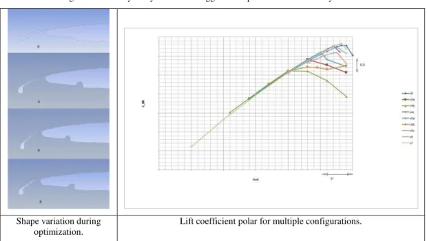
For every major shape change (Fig. 7) the step that concerns the positioning optimization is reiterated such that a new setting for gap, overlap and deflection angle that maximizes the lift to drag ratio as well as the AoA at which the stall is obtained.

Fig. 6 – Sensitivity analysis results. Suggested displacement indicated by arrows.

Shape variation during optimization.

Lift coefficient polar for multiple configurations.

Fig. 7 – Krueger flap shape change in the optimization process. Lift polar for various configurations.

(7)

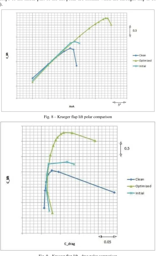
the same error/deviation in all the results. It is worth mentioning that the slight modifications of the slope of the linear part of the lift polar are normal when the Krueger flap is deployed (Fig. 8).

Fig. 8 – Krueger flap lift polar comparison

(8)

4. CONCLUSIONS

A complex optimization algorithm has been presented for a 2D airfoil with a leading edge high lift device. The method is demonstrated for a realistic configuration at relevant Mach and Reynolds numbers. The results of the method are verified on a very fine mesh and presented in a comparative manner with the results obtained using the same approximations for the clean airfoil and show enhanced aerodynamic performances, similar to what one would expect from a leading edge slat.

The use of the gliding ratio as the optimization criteria is justified and the apparently more intuitive and simple use of lift is dismissed and explained. Another possibility that remains to be further investigated is the use as an optimization target of the gliding ratio at a power higher than 1; that is to give the lift’smaximization a higher influence over the drag’s minimization.

The methodology can be easily extrapolated to 2.5D and 3D configurations while taking into account the constraint coming from the work effort for the 3D configurations.

REFERENCES

[1] B. Soemarwoto, The Variational Method for Aerodynamic Optimization Using the Navier-Stokes Equations,

ICASE – Technical report, 1997.

[2] H. Farrokhfal, A. R. Pishevar, Aerodynamic shape optimization of hovering rotor blades using a coupled free wake–CFD and adjoint method, Aerospace Science and Technology, vol. 28, pp 21–30, Issue 1, 2013. [3] D.Jones, J.-D. Müller, F. Christakopoulos, Preparation and assembly of discrete adjoint CFD codes,

Computers and Fluids, vol. 46, pp. 282-286, 2011.

[4] Q.-Z. Yang, Z.-Y. Zhang, S. Thomas, W. Georg, Y. Zheng, Aerodynamic Design for Three- Dimensional Multi- lifting Surfaces at Transonic Flow, Chinese Journal of Aeronautics, vol. 19, pp. 24-30, 2006. [5] J. Brezillon, N. R. Gauger, 2D and 3D aerodynamic shape optimisation using the adjoint approach, Aerospace