Response of OH airglow emissions to the mesospheric gravity waves and its comparisons with full wave model simulation at a low latitude Indian station

(1)

ACPD

15, 35881–35906, 2015

Characterization of gravity waves using

OH airglow investigation

R. N. Ghodpage et al.

Title Page

Abstract Introduction

Conclusions References

Tables Figures

◭ ◮

Back Close

Full Screen / Esc

Printer-friendly Version Interactive Discussion

Discussion

P

a

per

|

Discussion

P

a

per

|

Discussion

P

a

per

|

Discussion

P

a

per

|

Atmos. Chem. Phys. Discuss., 15, 35881–35906, 2015 www.atmos-chem-phys-discuss.net/15/35881/2015/ doi:10.5194/acpd-15-35881-2015

This discussion paper is/has been under review for the journal Atmospheric Chemistry and Physics (ACP). Please refer to the corresponding final paper in ACP if available.

Response of OH airglow emissions to the

mesospheric gravity waves and its

comparisons with full wave model

simulation at a low latitude Indian station

R. N. Ghodpage1, M. P. Hickey2, A. Taori3,a, D. Siingh4, and P. T. Patil1

1

Indian Institute of Geomagnetism, Shivaji University Campus, Kolhapur 416004, India

2

Embry-Riddle Aeronautical University, FL 32114, USA

3

National Atmospheric Research Laboratory, Pakala Mandal, Gadanki (A. P.) 517112, India

4

Indian Institute of Tropical Meteorology, Pune-411 008, Maharashtra, India

a

now at: National Remote Sensing Center (NRSC), Hyderabad, 500037, India

Received: 12 October 2015 – Accepted: 8 December 2015 – Published: 21 December 2015

Correspondence to: A. Taori (alok.taori@gmail.com)

(2)

ACPD

15, 35881–35906, 2015

Title Page

Tables Figures

◭ ◮

Back Close

Full Screen / Esc

Discussion

P

a

per

|

Discussion

P

a

per

|

Discussion

P

a

per

|

Discussion

P

a

per

|

Abstract

The quasi-monochromatic gravity wave induced oscillations, monitored using the mesospheric OH airglow emission over Kolhapur (16.8◦N and 74.2◦E), India during January to April 2010 and January to December 2011, have been characterized using the Krassovsky method. The nocturnal variability reveals prominent wave signatures

5

with periods ranging from 5.2–10.8 h as the dominant nocturnal wave with embedded short period waves having wave periods 1.5–4.4 h. The results show that the magni-tude of the Krassovsky parameter, viz.,|η|ranged from 2.1 to 10.2 for principal or long nocturnal waves (5.2 to10.8 h observed periods), and, from 1.5 to 5.4 for the short waves (1.5 to 4.4 h observed periods) during the years of 2010 and 2011, respectively.

10

The phase, i.e.,Φ_{values of the Krassovsky parameters exhibited larger variability and}

varied from−8.1 to −167◦. The deduced mean vertical wavelengths are found to be approximately −60.2±20 and −42.8±35 km for long and short wave periods for the year 2010. Similarly, for 2011 the mean vertical wavelengths are found to be approxi-mately−77.6±30 km and−59.2±30 km for long and short wave periods, respectively,

15

indicating that the observations over Kolhapur were dominated by upward propagat-ing waves. We use a full wave model to simulate the response of OH emission to the wave motion and compare the results with observed values. In the present report, we discuss the observed wave characteristics and cause of the noted diff_erences.

1 Introduction 20

Often the observed temporal variations in the mesospheric hydroxyl OH night airglow intensities and rotational temperatures are caused by the propagating gravity waves from the lower to the upper atmosphere. The interaction of these upward propagating waves with the ambient and other waves contribute to the dynamical variability, which in turn is reflected in observed airglow intensity and temperature perturbations (Hines,

25

(3)

ACPD

15, 35881–35906, 2015

Title Page

Tables Figures

◭ ◮

Back Close

Full Screen / Esc

Discussion

P

a

per

|

Discussion

P

a

per

|

Discussion

P

a

per

|

Discussion

P

a

per

|

perturbations. This parameter, termed as “Krassovsky’s parameter”, can be defined as η=_|_η_|_e−iΦ_{, where} _|_η_|_{indicates the ratio of the amplitude variation between the}

emis-sion intensity and temperature perturbations normalized to their time averages andΦ

is a phase diff_{erence between the intensity wave and its temperature counterpart (e.g.,}

Walterscheid et al., 1987; Taylor et al., 1991). It should also be mentioned here that

5

apart from the pure dynamical processesηcan also be aff_{ected by various other}

un-known parameters, such as the variation of local oxygen photochemistry (Hickey et al., 1993) and height variation of the emission layer which aff_{ects emission rates and}

tem-perature directly (Liu and Swenson, 2003; Vargas et al., 2007). Although this can com-plicate studies of Krassovsky’s parameter, it off_{ers an opportunity to study the above} 10

aspects at the same time. Overall, once the physics and chemistry of emissions are well understood, theηvalues would off_{er a good tool to study the perturbations caused}

in a parameter (temperature, brightness/intensity) by measuring one under adiabatic conditions.

Utilizing the above, many investigators have carried out observational as well as

15

the theoretical studies on the identification and characterization of gravity wave and tidal signatures with wave periodicities ranging from few minutes to several hours (e.g., Walterscheid et al., 1987; Hecht et al., 1987; Hickey, 1988a, b; Taylor et al., 1991; Takahashi et al., 1992; Reisin and Scheer, 1996; Taori and Taylor, 2006; Guharay et al., 2008; Ghodpage et al., 2012, 2013). However, observational studies of the magnitude

20

and phase ofηover a range of wave periods for a given location and season are sparse. Some of the notable observations ofη for the OH emission have been performed by Viereck and Deehr (1989) in the wave period range of ∼1–20 h and by Reisin and Scheer (1996) near to the semidiurnal tidal fluctuations.

In the present work, we utilize the mesospheric OH emission intensity and

temper-25

(4)

ACPD

15, 35881–35906, 2015

Title Page

Tables Figures

◭ ◮

Back Close

Full Screen / Esc

Discussion

P

a

per

|

Discussion

P

a

per

|

Discussion

P

a

per

|

Discussion

P

a

per

|

estimates with the earlier results reported by various investigators. We also employ a full-wave model to simulate the eff_{ects of wave motions on the OH airglow. This model}

has been used previously to compare observations and theory of airglow fluctuations (e.g., Hickey et al., 1998; Hickey and Yu, 2005). Here, the model is used to estimate the values of the amplitudes and phases of Krassovsky’s ratio which are compared to

5

those derived from the observations, making the present study unique and the first of its kind over Indian latitudes.

2 Instrumentation and observations

The mesospheric OH observations used in the present study are made using the mul-tispectral photometer from Kolhapur (16.8◦N, 74.2◦E) (Ghodpage et al., 2013, 2014).

10

We use the period of January–April 2010 and January–December 2011 when the avail-ability of clear sky conditions prevailed for several nights. In particular, for 2010 data, out of 45 nights of OH airglow measurements, 14 nights clearly showed wavelike features, while in the 2011 year data, 60 nights out of 30 nights exhibited wavelike variations.

2.1 The multispectral photometer 15

The multi-spectral photometer monitors airglow emissions at 731 and 740 nm rotational lines of OH (8,3), O(1S) 557.7 nm and O(1D) 630.0 nm emissions near simultaneously. The low temperature coeffi_{cient interference filters (10 cm aperture) used in the}

pho-tometer have full width at half maximum ∼1 nm (transmission ∼40–70 % at 24◦C). We kept the integration time for each filter 10 s which results in repetition time of 90 s.

20

(5)

ACPD

15, 35881–35906, 2015

Title Page

Tables Figures

◭ ◮

Back Close

Full Screen / Esc

Discussion

P

a

per

|

Discussion

P

a

per

|

Discussion

P

a

per

|

Discussion

P

a

per

|

of nA) output current in to corresponding voltage form. This output is recorded in digital format in term of arbitrary units along with time which is used for further processing.

2.2 Full-wave model

The full-wave model is a linear, steady-state model that solves the linearized Navier– Stokes equations on a high resolution vertical grid to describe the vertical

propaga-5

tion of acoustic-gravity waves in a windy background atmosphere including molecular viscosity and thermal conduction, ion drag, Coriolis force and the eddy diff_{usion of}

heat and momentum in the mesosphere. The model description, including equations, boundary conditions and method of solution has been described elsewhere (Hickey et al., 1997; Walterscheid and Hickey, 2001; Schubert et al., 2003). The neutral

per-10

turbations are used as input to a linear, steady-state model describing OH airglow fluctuations (Hickey and Yu, 2005).

The model solves the equations on a high resolution vertical grid subject to bound-ary conditions, and allows quite generally for the propagation in a height vbound-arying atmo-sphere (non-isothermal mean state temperature and height varying mean winds and

15

diff_{usion). The linearized equations are numerically integrated from the lower to the}

upper boundary using the tri-diagonal algorithm described by Bruce et al. (1958) and Lindzen and Kuo (1969). The lower boundary is set well below the region of interest and a sponge layer is implemented to avoid eff_{ects of wave reflection in the airglow}

response. In this study the lower boundary (the bottom of the lower sponge layer) is

20

placed at 250 km below z=_{0 (i.e.,} _{−250 km). The wave forcing is through the}

addi-tion of heat in the energy equaaddi-tion. The heating is defined by a Gaussian profile with a full-width-at-half-max of 0.125 km. It is centered at an altitude of 10 km. A Rayleigh– Newtonian sponge layer in addition to natural absorption by viscosity and heat con-duction prevents spurious reflection from the upper boundary. At the upper boundary

25

(6)

ACPD

15, 35881–35906, 2015

Title Page

Tables Figures

◭ ◮

Back Close

Full Screen / Esc

Discussion

P

a

per

|

Discussion

P

a

per

|

Discussion

P

a

per

|

Discussion

P

a

per

|

A set of linear perturbation equations for the minor species involved in the OH emis-sion chemistry is solved using the approach described in Hickey (1988). This assumes that these minor species have the same velocity and temperature perturbations as the major gas (which are deduced from the full-wave model). A vertical integration of the volume emission rates through the vertical extent of the OH layer provides the

bright-5

ness and brightness-weighted temperature perturbations, from which Krassovsky’s ra-tio is determined. The OH chemistry we use is the same as that used previously (Hickey et al., 1997) and is for the OH (8–3) emission. We also determine the vertical wave-length at the peak of the OH emission layer evaluated from the phase variations of the temperature perturbations determined by the full-wave model.

10

2.3 Space borne measurements

The sounding of the atmosphere using broadband emission radiometry (SABER), on-board the thermosphere ionosphere mesosphere energetic and dynamics (TIMED) satellite, is a high-precision broadband radiometer which measures limb radiance (at 74◦) of the terrestrial at in 10 selected spectral bands ranging from 1.27 to 15 µm. In

15

the present study, we note larger values of |η| occur during 2011 compared to 2010 for long/principal waves, which indicates a larger intensity to temperature perturbation ratio over Kolhapur during the passage of the waves during 2011. This could be due to the diff_{erences in either the background atmosphere or the dynamical processes}

of 2010 and 2011 years. To identify this, we scrutinize the OH volume emission rate

20

profile for Kolhapur region (obtained from the SABER instrument on-board the thermo-sphere ionothermo-sphere mesothermo-sphere energetic and dynamics (TIMED) satellite). The se-lected latitude–longitude grids are 10 to 20◦N and 70 to 90◦E representing Kolhapur. The criteria for the selection of SABER data are such that: (i) the SABER pass should be during typical observation times (i.e. nighttime), (ii) it should not be at twilight.

(7)

ACPD

15, 35881–35906, 2015

Title Page

Tables Figures

◭ ◮

Back Close

Full Screen / Esc

Discussion

P

a

per

|

Discussion

P

a

per

|

Discussion

P

a

per

|

Discussion

P

a

per

|

3 Results and discussion

To identify the wave structures in the data, we utilize the perturbation amplitudes nor-malized to their time averaged values (hereafter referred to as mean values) in the intensity and temperature data to calculate the Krassovsky ratio. To illustrate this, we show a typical example corresponding to the data obtained on 26–27 January 2011

5

in Fig. 1. We plot the temperature deviations (circles with connecting lines) from their mean values in Fig. 1a, while, the intensity deviations (circles with connecting lines) from their mean values are plotted in Fig. 1b. We note that night airglow intensity vari-ations show a long-period wave with embedded short-period oscillatory features. On this night, the mean of airglow intensity is found to be∼1.83 arbitrary units and the

10

mean of the temperature data is∼195.75 K. To identify the nocturnal variability plotted together with data are the results (shown as red solid lines) of best-fit cosine model (e.g., Taori et al., 2005) as follows.

Y =_A_cos

π(X−Xc) T

(1)

where,Ais the amplitude of the fitted wave of half-periodT with phase Xc, andX is the

15

time. Note that the solid red lines in Fig. 1 show the results of the best-fit cosine model. We observed the presence of∼8.2±1.1 and 8±1.3 h waves with relative amplitudes ∼7.57 and 54.5 %, in the nocturnal temperature and intensity variability, respectively. Given the uncertainties involved in the observations, we consider these to be the same waves. Further, we compute the|η|value for this wave to be 7.2±1.3. To identify the

20

shorter period features in the data we obtain residuals from the best-fit model values (Fig. 1c). The bottom-left (Fig. 1c) and bottom-right (Fig. 1d) panels show the nocturnal variability of the residual temperature and intensity, respectively. The best-fit model re-veals the presence of∼4.0±0.2 and 3.0±0.8 h wave in the temperature and intensity residuals, respectively. Once again we treat these as the same wave for the reason

ex-25

(8)

ACPD

15, 35881–35906, 2015

Title Page

Tables Figures

◭ ◮

Back Close

Full Screen / Esc

Discussion

P

a

per

|

Discussion

P

a

per

|

Discussion

P

a

per

|

Discussion

P

a

per

|

Hence, the|η|value for short period waves is estimated to be 3.7±0.9. The phase diff

er-ence between the intensity and temperature waves is obtained with the help of best-fit parameters which were also verified with a cross correlation analysis. The phase of the principal waves (maxima) (period ∼8.2 h) was∼25.02 h in the temperature data and 24.6 h in the intensity data, which results in the phase diff_{erence of}_∼_{0.4 h, i.e.,}Φ 5

values of−18.0±10◦. Similarly, for the shorter period (period∼4 h) theΦ _{values are}

estimated to be−100.8±22◦.

We can also estimate the vertical wavelength with the help of Krassovsky’s parame-ter following the approach of Tarasick and Hines (1990):

λz= 2πγH

(γ−1)|η|sin(ϕ) (2)

10

whereγ=_C_p_/C_v=_{1.4 is the ratio of specific heats, and}_H=_{6 km is the scale height.}

This formula is valid for zenith observations and for plane waves. It is not valid for the evanescent waves. Using the above relation we find that vertical wavelength for the two cases discussed above are∼ −39±15 and−35.5±10 km for long period and short period waves, respectively. Note that the long period wave estimates may be

15

biased when the data length is comparable to that of the wave period and therefore in our study we have considered only those waves whose periods are substantially less than the length of the available data.

The above analysis was carried out on nighttime events recorded during 2010 and 2011 when the prominent wave features were visible. One may note that during the

20

2010 period, the principal nocturnal waves in the data show the wave periods vary from 5.2 to 10.8 h with corresponding temperature amplitudes ranging from 0.2 to 13.8 K. Similarly for 2011, wave periods vary between 5.2 and 8.4 h with corresponding tem-perature amplitudes lying between 0.7 and 15.7 K. However, the intensity amplitudes of the principal waves vary from 1.5 % to 56.5 and 5 to 90 % for 2010 and 2011,

re-25

(9)

ACPD

15, 35881–35906, 2015

Title Page

Tables Figures

◭ ◮

Back Close

Full Screen / Esc

Discussion

P

a

per

|

Discussion

P

a

per

|

Discussion

P

a

per

|

Discussion

P

a

per

|

4.4 h (for 2010) and 2.8 to 4.4 h (for 2011) with corresponding temperature amplitudes ranging from 0.2 to 12.5 and 0.4 to 14.4 K. The corresponding intensity amplitudes varied from∼1.8 to 56 and 0.8 to 46.8 % for 2010 and 2011, respectively. The phase (Φ_{) values also exhibit large variability for long (short) period waves, varying between}

−27 and−167◦ (−27 and−150◦) for 2010 and−8.1 and −65.2◦ (−39.1 and −122.6◦)

5

for 2011. For 2010 the deduced vertical wavelengths are found to vary from−32.2 to −140 and −24 to −88 km for the long and short period waves, respectively. Similarly, for 2011 the deduced vertical wavelengths are found to vary from −40 to −102, and −26 to−92.4 km for the long and short period waves, respectively.

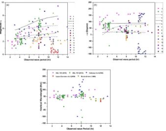
In Fig. 2a we plot our results for|η|(hereafterη) with pink half-filled squares indicating

10

the estimates for the year 2010 and olive half-filled squares for the year 2011. We plot Φ _{in Fig. 2b using the same symbols as used in Fig. 2a. For a comparison, we}

also show the values ofηandΦ _{reported by other investigators (Viereck and Deehr,}

1989; Takahashi et al., 1992; Oznovich et al., 1995, 1997; Drob, 1996; Reisin and Scheer, 1996; Taylor et al., 2001; Lopez-Gonzalez et al., 2005). Also shown in the figure

15

are the model estimates of Schubert et al. (1991), Tarasick and Shepherd (1992a, b), Walterscheid and Schubert (1995). In general, we observe that the parameter η increases with wave period. It is evident that the observedηandΦ_{values in our study}

show a large spread in their distribution as compared to the model values. A similar spread in the distribution of observed values ofη(Fig. 2a) from 1.03 to 7.85 has also

20

been observed by other investigators (e.g., Takahashi et al., 1992). It may be noted that the values of ηfor the OH data in our study lie somewhere between the model estimates and the values observed by other investigators. Also noteworthy in this figure is that ourηvalues are closer to the model values reported by Tarasick and Shepherd (1992a) for the waves with horizontal wavelength 500 km. The phase “Φ_{” values, on} 25

the other hand show significantly larger deviations from this model for 2010, while for 2011 the match between measured and modeled phases appear to be better. We note that our measurements ofΦ _{matches somewhat with those reported by Viereck and}

(10)

ACPD

15, 35881–35906, 2015

Title Page

Tables Figures

◭ ◮

Back Close

Full Screen / Esc

Discussion

P

a

per

|

Discussion

P

a

per

|

Discussion

P

a

per

|

Discussion

P

a

per

|

variation of Φ _{values with respect to the wave periodicity, obtained in the 2010 year}

clearly shows that most of the time we observe values to be higher than those obtained by diff_{erent models.}

In particular, Reisin and Scheer (1996) found mean (arithmetic) value of η to be 5.5±0.6 and the mean Φ_{value to be} ₋₆₆◦ _{for OH. Our observed values of} _η (arith-5

metic mean, 4.4±1 for 2010 year and 5.7±1.7 for 2011 year) near by agree with the values reported by Reisin and Scheer (1996) for OH measurements. In a further report, based on 5 year observations, Reisin and Scheer (2004), found the mean value of η to be∼5.6 for the nightly semidiurnal type waves and ∼3.4 for the waves of 3000 s periodicity; which is in agreement with our values. In another study based on long-term

10

observations with a spectral airglow temperature imager (SATI) from a mid-latitude sta-tion, Lopez-Gonzalez et al. (2005) reported a mean value ofηof approximately∼8.6 for the OH measurements with a larger variability than our observations show. In an-other report, Guharay et al. (2008), found that for wave periods ranging from 6 to 13 h, values ofηvaried from 1.7 to 5.4, while the phase varied from−13 to−90◦. Similarly,

15

Aushev et al. (2008) presented amplitudes of the Krassovsky parameter for wave pe-riods of 2.2 to 4.7 h which varied from 2.4 to 3.6 while the phase varied from−63 to −121◦. It is noteworthy that our derived values broadly agree with Guharay et al. (2008, 2009), Reisin and Scheer (1996, 2004) and Viereck and Deehr (1989) while they are somewhat diff_{erent from the values reported by Lopez-Gonzalez et al. (2005) (which} 20

may be due to the fact that their observations corresponded to higher latitude than ours).

In general, the results shown in Fig. 2 emphasize that there are significant in the Krassovsky parameters derived from one study to another. This we suspect to be caused by the variations in the altitudinal profile of oxygen and its eff_{ect on the} _η 25

(11)

lev-ACPD

15, 35881–35906, 2015

Title Page

Tables Figures

◭ ◮

Back Close

Full Screen / Esc

Discussion

P

a

per

|

Discussion

P

a

per

|

Discussion

P

a

per

|

Discussion

P

a

per

|

els. Winds also aff_{ect the OH response to gravity waves and therefore they will also}

contribute to the spread of values seen between the various observation studies. Note that our observations as well as models show the phaseΦ_{for OH to be a}

neg-ative value indicating the upward propagating waves. In general we note that our Φ

values, although on some occasions are closer to Viereck and Deehr (1989)

obser-5

vations, show large deviations from other investigators and are larger than the model values on most occasions. Diff_{erences in theory and observation may be due to the}

hor-izontal wavelength assumed in the model and or the Prandtl number (ratio of kinematic viscosity to thermal diff_{usivity) assumed. The Prandtl number is important in}

theoret-ical calculations and modeling, especially when in terms of dissipating waves owing

10

to molecular viscosity and thermal diff_{usivity while they propagate in the atmosphere}

(Hickey, 1988). An error in the Prandtl number assumption will aff_{ect the derived wave}

parameters (λ_z,η etc.), which will successively mask the actual ones. In this regard, Makhlouf et al. (1995) studied the variations in theη values by modifying the model proposed by Hines and using a photochemical dynamical model; however, they were

15

still unable to explain the appearance of the negative phases appropriately. Hines and Tarasick (1987) found a wide range of η variability, a result supported by our mea-surements. Further, Hines and Tarasick (1997) subsequently discussed the necessary correction for thin and thick layer approximations for the calculation ofηfrom airglow emissions due to gravity waves interaction. They also pointed out that OH emission

20

intensity, which aff_{ects the derived} _η _{values, does not depend on the oxygen profile}

and other minor species, which contradicts the theory of Walterscheid et al. (1994), Schubert et al. (1991) and Off_{ermann et al. (1981).}

The calculated vertical wavelengths (VW) for all the nights of the observation are shown in Fig. 2c as pink half filled squares indicating the estimates for the year 2010

25

and olive half filled squares for the year 2011. Large diff_{erences exist from one night to}

(12)

ACPD

15, 35881–35906, 2015

Title Page

Tables Figures

◭ ◮

Back Close

Full Screen / Esc

Discussion

P

a

per

|

Discussion

P

a

per

|

Discussion

P

a

per

|

Discussion

P

a

per

|

years, the mean VW values for long and short period waves are calculated to be −60.2±20 km (−77.2±40 km) and−42.8±15 km (−59.2±30) respectively. All the ob-servations show negative values forΦ _and _λ_z_{, indicating upward propagating waves.}

Further, unlike the clear dependency on the wave period noted in the Krassovaky pa-rameters (ηandΦ_{) no clear trend is noted in the calculated VW. We also plot the values} 5

reported by Reisin and Scheer (1996) and Lopez-Gonzalez et al. (2005) for a compari-son. It is noteworthy that for all the days the VW for the long period wave are higher than the VW of short period waves. We also observed that VW values calculated for 2011 year are larger than 2010 year calculated values.We note that the values reported by Reisin and Scheer (1996) are approximately−30 km with about 40 km variability, which

10

is a good agreement with our values. However, Lopez-Gonzalez et al. (2005) observed VW values to be approximately−10 km deduced from their OH observations, which do not agree with our values. Further, Ghodpage et al. (2012) analyzed the long-term nocturnal data of 2004–2007 and also observed that the VW lies between 28.6 and 163 km. Recently, Ghodpage et al. (2013) studied the simultaneous mesospheric

grav-15

ity wave measurements in the OH emission from Gadanki and Kolhapur, inferring mean VWs varying from−26 to−60 km for the Kolhapur observations. Takahashi et al. (2011) reported vertical wavelengths varying from 20 to 80 km, which is in agreement with our values.

4 Comparison with the full wave model results 20

Wave simulations were performed using the full-wave model (FWM). The observa-tions were conducted over an approximate one month period spanning 8 February and 13 March, and accordingly we used the middle date of this observation period (25 February) in the MSIS model to represent the undisturbed mean state. The latitude used was 16.8◦N, and the local time was midnight. Because the speed and direction

25

(13)

ACPD

15, 35881–35906, 2015

Title Page

Tables Figures

◭ ◮

Back Close

Full Screen / Esc

Discussion

P

a

per

|

Discussion

P

a

per

|

Discussion

P

a

per

|

Discussion

P

a

per

|

northward and westward propagation) and the phase speed (50, 100 and 150 m s−1) were varied. Note that the mean winds (not shown) in these simulations were derived from the Horizontal Wind Model (HWM) using the same input parameters as used for the MSIS model. The derived meridional winds (not shown) are far smaller than the zonal winds for the conditions considered here, and so while results for eastward and

5

westward propagation diff_{ered quite markedly, those for northward and southward}

prop-agation did not. Hence we considered only a single direction (northward) for meridional propagation.

We also performed a tidal simulation using an equivalent gravity wave model (Lindzen, 1970; Richmond, 1975), as implemented in an earlier study (Walterscheid

10

and Hickey, 2001). The horizontal wavelength and Coriolis parameter are adjusted to give maximal correspondence with a given tidal mode. Here, we performed calcula-tions for the terdiurnal (3,3), (3,4), (3,5) and (3,6) modes using parameters provided by Richmond (1975). The simplifications inherent in this approach are discussed by Walterscheid and Hickey (2001).

15

Comparisons between the full wave model results for η, Φ _and _λ_z _{and the values}

inferred from the observations are shown in Fig. 3a–c, respectively. In Fig. 3a we com-pare the observed values ofηfor 2010 and 2011. show The observed values ofηare represented as pink and olive lower half-filled squares for 2010 and 2011, respectively. In Fig. 3a we note that at few of the longer wave periods, the observed values ofηare

20

in good agreement with the full wave model results. For short period waves the val-ues ofηinferred from the observations appear to be bounded by the model values for waves with horizontal phase velocities are 50–100 m s−1, respectively. For example, for 3.6 h wave periods, the average of the values ofηinferred from the observations is 3.7, while the full wave model values lie between about 0.5 (for the 100 m s−1wave) and 7

25

(for the 50 m s−1, eastward propagating wave). For the 8 h wave periods, the average of the values ofηinferred from the observations is 5.7, which is bounded by the full wave model estimates for waves having a horizontal phase velocity of 50 m s−1and diff_erent

(14)

ACPD

15, 35881–35906, 2015

Title Page

Tables Figures

◭ ◮

Back Close

Full Screen / Esc

Discussion

P

a

per

|

Discussion

P

a

per

|

Discussion

P

a

per

|

Discussion

P

a

per

|

Overall, we note that that the comparison between the observedη values and the modeled values can be explained by gravity waves whose horizontal phase velocities range from 50 to 100 m s−1. In this regard, an earlier investigation by Pragati Sikha et al. (2010) reported observed gravity wave horizontal phase speeds (for periods 5 to 17 min) varying between 10 and 48 m s−1. The propagation directions were reported

5

to be preferentially towards the north. More recently, Taori et al. (2013) studied meso-spheric gravity wave activity in the OH and OI 558 nm emissions from Gadanki. They observed that the gravity waves were moving in the north-west direction. The average phase velocity of the ripple-type waves was found to be 23.5 m s−1. The other, band-type waves, with horizontal scales of about 40 km, were found to be propagating from

10

south to north with an estimated phase speed of 90 m s−1.

The vertical wavelengths (λ_z) calculated using the observed values ofηandΦ_diff_er

significantly from the full wave model estimate for waves with phase velocities below 100 m s−1. More typically, a comparison between those values inferred from the ob-servations and those derived from the model tend to agree for phase velocities in the

15

100–150 m s−1 range. However, it should be noted that vertical wavelengths inferred from the observations are based on the use of the inferred Krassovsky’s ratio, η, in Eq. (2). Errors in the determination of the phase (Φ_{) of}_η_{can lead to significant errors}

(proportional to cotΦ_{) in the determination of}_λ_z_{, especially as}Φ_approaches_±180◦_.

The diff_{erences noted in the observed and modeled estimates of Krassovsky} ra-20

tio magnitudes ηand phase (Φ_{) may be associated with the limitation arising due to}

dynamics as well as the measurements. In terms of measurements limitation, the pa-rameters achieved with the best fit method may have leaked contribution from other wave components which may be dynamically varying within a wave period. In terms of dynamics, that full wave model uses climatological density (both major gas and minor

25

airglow-related species) and wind profiles which will introduce uncertainties. This point has been previously elaborated by Walterscheid et al. (1994) with respect to the eff_ect

(15)

ACPD

15, 35881–35906, 2015

Title Page

Tables Figures

◭ ◮

Back Close

Full Screen / Esc

Discussion

P

a

per

|

Discussion

P

a

per

|

Discussion

P

a

per

|

Discussion

P

a

per

|

The diff_{erences noted in the magnitude of the observed Krassovsky ratio}_η_between

2010 and 2011 may be associated with variations in the height and shape of the undis-turbed OH emission profile. To check whether there was a diff_{erence in the OH}

emis-sion layer structure, we selected the nighttime OH emisemis-sion profile for a grid encom-passing 10 to 20◦N latitudes and 70 to 90◦E latitudes during February, March and April

5

months of the years 2010 and 2011. We have selected the February to March period because the optical airglow data used in this study was acquired primarily during these months. The monthly mean values of OH emission rates are plotted in Fig. 4. The solid curves correspond to 2010 data while the dashed curves correspond to 2011 data for. We note that the peaks of OH emission layer during February, March and April of

10

2010 occurred at 84.2, 82.8 and 85.1 km altitude, respectively, while the corresponding peaks for 2011 were found to occur at 85.8, 85.6 and 85.2 km altitude. This suggests that the peak of the emission layer occurred at a somewhat lower altitude in 2010 com-pared to 2011. Also, the mission rates during February and March were found to be higher in 2010. It is important to note that in an earlier study, Ghodpage et al. (2013)

15

compared the Krassovsky ratios at two diff_{erent latitudes, Gadanki (13.5}◦_{N, 79.2}◦_E)

and Kolhapur (16.8◦N and 74.2◦E) and noted a lower OH emission layer peak over Kolhapur and also larger estimated η values over Kolhapur. In the present case, in-stead of the location, it is the diff_{erence in the measurement year where the peak}

emission altitudes of the OH emission layer are somewhat diff_{terent. As the peak} emis-20

sion layer arise due to the chemical reactions involving odd oxygen, it is proposed that chemical constutents composition were diff_{erent from the year 2010 to the year}

2011. Therefore, the noted emission rates may be responsible for the observed diff

er-ences in the Krassovsky parameters. A further question arise here is why the peaks should be diff_{erent from one year to the other. As these months are pre-monsoon, when} 25

(16)

ACPD

15, 35881–35906, 2015

Title Page

Tables Figures

◭ ◮

Back Close

Full Screen / Esc

Discussion

P

a

per

|

Discussion

P

a

per

|

Discussion

P

a

per

|

Discussion

P

a

per

|

months in 2011. We postulate that these large scale processes have a profound im-pact on the observed wave energetics and dynamics at mesospheric altitudes. Large scale processes induced the wave oscillations associated with the ENSO. The ENSO generates a spectrum of waves which are of planetary scales. These are expected to generate a secular variation in temperature and density structure throughout the

atmo-5

sphere. A diff_{erence in ENSO suggests that these forcing are di}ff_{erent in the two years}

(2010, 2011). At present, we do not know through which process the ENSO may have implications in the observed wave characteristics. However, we believe that further in-vestigation is required in order to confirm whether or not any such associations really do exist.

10

5 Concluding remarks

We report the Krassovsky parameters for the observed gravity waves from Kolhapur (16.8◦N and 74.2◦E) and their comparison with the full wave model. Following are the concluding remarks of the present investigations.

1. It is evident that the observed values of Krassovsky parameters in our study show

15

a large spread in their distribution as compared to the model values (shown in Fig. 2a). A similar spread in the distribution has also been reported by other in-vestigators. We have also observed that more magnitude ofηvalues in 2011 year than 2010 year.

2. It is also notable that the values ofηfor the OH data in our study lie between the

20

model estimates and the values observed by other investigators. Whereas the phase values are more than the model values on most occasions. We note that our Φ _{measurements match with those reported by Viereck and Deehr (1989),}

while they show large diff_{erences with other investigators values.}

3. Observed vertical wavelength (VW) values broadly agree with the range reported

25

(17)

ACPD

15, 35881–35906, 2015

Title Page

Tables Figures

◭ ◮

Back Close

Full Screen / Esc

Discussion

P

a

per

|

Discussion

P

a

per

|

Discussion

P

a

per

|

Discussion

P

a

per

|

that VW values calculated for 2011 year are larger than 2010 year calculated values. Most of wave propagating upward in direction.

4. Comparison of observedηandΦ_{values agree fairly well with the full wave model}

results for waves with 50–100 m s−1 horizontal phase velocities. Vertical wave-lengths tend to agree for waves with 100–150 m s−1 horizontal phase velocities,

5

except for the longest period waves for which vertical wavelength cannot be reli-ably inferred from the observations.

The database used in the present study is limited in terms of the length and locations and based on the above conclusions, more rigorous study using coordinated observa-tions and modeling are underway with an aim to uncover the physics occurring at upper

10

mesosphere.

Acknowledgements. This work is carried out under the research grant funded by Ministry of Science and Technology and Department of Space, Govt. of India. R. N. Ghodpage thank the Director, Indian Institute of Geomagnetism (IIG), Navi Mumbai for encouragement to carry out this work. The night airglow observations at Kolhapur were carried out under the

scien-15

tific collaboration program (MoU) between IIG, Navi Mumbai and Shivaji University, Kolhapur. M. P. Hickey acknowledges the support of NSF grant AGS-1001074.

References

Aushev, V. M., Lyahov, V. V., Lopez-Gonzalez, M. J., Shepherd, M. G., and Dryna, E. A.: Solar eclipse of the 29 March 2006: results of the optical measurements by MORTI over Almaty

20

(43.03◦N, 76.58◦E), J. Atmos. Sol.-Terr. Phy., 70, 1088–1101, 2008.

Bruce, G. H., Peaceman, D. W., Rachford Jr., H. H., and Rice, J. D.: Calculations of unsteady-state gas flow through porous media, Petrol. Trans. AIME, 198, 79–92, 1953.

Drob, D. P.: Ground-based optical detection of atmospheric waves in the upper mesosphere and lower thermosphere, PhD thesis, University of Michigan, Ann Arbor, MI, 1996.

25

(18)

ACPD

15, 35881–35906, 2015

Title Page

Tables Figures

◭ ◮

Back Close

Full Screen / Esc

Discussion

P

a

per

|

Discussion

P

a

per

|

Discussion

P

a

per

|

Discussion

P

a

per

|

Ghodpage, R. N., Taori, A., Patil, P. T., and Gurubaran, S.: Simultaneous mesospheric gravity wave measurements in OH night airglow emission from Gadanki and Kolhapur – Indian low latitudes, Curr. Sci. India, 104, 1, 98–105, 2013.

Ghodpage, R. N., Taori, A., Patil, P. T., Gurubaran, S., Sharma, A. K., Nikte, S., and Nade, D.: Airglow measurements of gravity wave propagation and damping over Kolhapur (16.8◦N,

5

74.2◦E), Int. J. Geophys., 2014, 1–9, doi:10.1155/2014/514937, 2014.

Guharay, A., Taori, A., and Taylor, M.: Summer-time nocturnal wave characteristics in meso-spheric OH and O₂airglow emissions, Earth Planets Space, 60, 973–979, 2008.

Guharay, A., Taori, A., Bhattacharjee, B., Pant, P., Pande, P., and Pandey, K.: First ground-based mesospheric measurements from central Himalayas, Curr. Sci. India, 97, 664–669,

10

2009.

Hecht, J. H., Walterscheid, R. L., Sivjee, G. G., Christensen, A. B., and Pranke, J. B.: Ob-servations of wave-driven fluctuations of OH nightglow emission bfrom Sondre Stromfjord, Greenland, J. Geophys. Res., 92, 6091–6099, 1987.

Hedin, A. E.: Extension of the MSIS thermosphere model into the middle and lower

atmo-15

sphere, J. Geophys. Res., 96, 1159–1172, 1991.

Hickey, M. P.: Effects of eddy viscosity and thermal conduction and coriolis force in the dynamics of gravity wave driven fluctuations in the OH nightglow, J. Geophys. Res., 93, 4077–4088, 1988.

Hickey, M. P. and Cole, K. D.: A quartic dispersion equation for internal gravity waves in the

20

thermosphere, J. Atmos. Terr. Phys., 49, 889–899, 1987.

Hickey, M. P. and Yu, Y.: A full-wave investigation of the use of a “cancellation fac-tor” in gravity wave-OH airglow interaction studies, J. Geophys. Res., 110, A01301, doi:10.1029/2003JA010372, 2005.

Hickey, M. P., Schubert, G., and Walterscheid, R. L.: Gravity wave-driven fluctuations in the

25

O₂atmospheric (0–1) nightglow from an extended, dissipative emission region, J. Geophys. Res., 98, 13717–13730, 1993.

Hickey, M. P., Walterscheid, R. L., Taylor, M. J., Ward, W., Schubert, G., Zhou, Q., Garcia, F., Kelley, M. C., and Shepherd, G. G.: Numerical simulations of gravity waves imaged over Arecibo during the 10-day January 1993 campaign, J. Geophys. Res., 102, 11475–11489,

30

1997.

(19)

ACPD

15, 35881–35906, 2015

Title Page

Tables Figures

◭ ◮

Back Close

Full Screen / Esc

Discussion

P

a

per

|

Discussion

P

a

per

|

Discussion

P

a

per

|

Discussion

P

a

per

|

Hickey, M. P., Huang, T. Y., and Walterscheid, R. L.: Gravity wave packet effects on chemical exothermic heating in the mesopause region, J. Geophys. Res., 108, 1448, doi:10.1029/2002JA009363, 2003.

Hines, C. O.: A fundamental theorem of airglow fluctuations induced by gravity waves, J. Atmos. Sol.-Terr. Phys., 59, 319–326, 1997.

5

Hines, C. O. and Tarasick, D. W.: On the detection and utilization of gravity waves in airglow studies, Planet. Space Sci., 35, 851–866, 1987.

Hines, C. O. and Tarasick, D. W.: Layer truncation and the Eulerian/Lagrangian duality in the theory of airglow fluctuations induced by gravity waves, J. Atmos. Sol.-Terr. Phys., 59, 327– 334, 1997.

10

Krassovsky, V. I.: Infrasonic variation of OH emission in the upper atmosphere, Ann. Geophys., 28, 739–746, 1972,

http://www.ann-geophys.net/28/739/1972/.

Lindzen, R. S.: Internal gravity waves in atmospheres with realistic dissipation and tempera-ture, part I: Mathematical development and propagation of waves into the thermosphere,

15

Geophys. Fluid Dyn., 1, 303–355, 1970.

Lindzen, R. S. and Kuo, H. L.: A reliable method for the numerical integration of a large class of ordinary and partial differential equations, Mon. Weather Rev., 97, 732–734, 1969. Liu, A. Z. and Swenson, G. R.: A modeling study of O₂and OH airglow perturbations induced

by atmospheric gravity waves, J. Geophys. Res., 108, 4151, doi:10.1029/2002JD002474,

20

2003.

López-González, M. J., Rodríguez, E., Shepherd, G. G., Sargoytchev, S., Shepherd, M. G., Aushev, V. M., Brown, S., García-Comas, M., and Wiens, R. H.: Tidal variations of O₂ atmo-spheric and OH(6-2) airglow and temperature at mid-latitudes from SATI observations, Ann. Geophys., 23, 3579–3590, doi:10.5194/angeo-23-3579-2005, 2005.

25

Makhlouf, U. B., Picard, R. H., and Winick, J. R.: Photochemical-dynamical modeling of the measured response of airglow to gravity waves, 1: basic model for OH airglow, J. Geophys. Res., 100, 11289–11311, 1995.

Offermann, D., Friedrich, V., Ross, P., and Von Zahn, U.: Neutral gas composition measure-ments between 80 and 120 km, Planet. Space Sci., 29, 747–764, 1981.

30

(20)

ACPD

15, 35881–35906, 2015

Title Page

Tables Figures

◭ ◮

Back Close

Full Screen / Esc

Discussion

P

a

per

|

Discussion

P

a

per

|

Discussion

P

a

per

|

Discussion

P

a

per

|

Oznovich, I., Walterscheid, R. L., Sivjee, G. G., and McEwen, D. J.: On Krassovsky’s ratio for ter-diurnal hydroxyl oscillations in the winter polar mesopause, Planet. Space Sci., 45, 385– 394, 1997.

Reisin, E. R. and Scheer, J.: Characteristics of atmospheric waves in the tidal period range derived from zenith observations of O₂(0–1) atmospheric and OH(6–2) airglow at lower mid

5

latitudes, J. Geophys. Res., 101, 21223–21232, 1996.

Reisin, E. R. and Scheer, J.: Gravity wave activity in the mesopause region from airglow mea-surements at El Leoncito, J. Atmos. Sol.-Terr. Phys., 66, 655–661, 2004.

Richmond, A. D.: Energy relations of atmospheric tides and their significance to approximate methods of solution for tides with dissipative forces, J. Atmos. Sci., 32, 980–987, 1975.

10

Schubert, G., Walterscheid, R. L., and Hickey, M. P.: Gravity wave-driven fluctuations in OH nightglow from an extended, dissipative emission region, J. Geophys. Res., 96, 13869– 13880, 1991.

Schubert, G., Hickey, M. P., and Walterscheid, R. L.: Heating of Jupiter’s thermosphere by the dissipation of upward propagating acoustic waves, Icarus, 163, 398–413, 2003.

15

Takahashi, H., Sahai, Y., Batista, P. P., and Clemesha, B. R.: Atmospheric gravity wave effect on the airglow O₂(0–1) and OH(9–4) band intensity and temperature variations observed from a low latitude station, Adv. Space Res., 12, 131–134, 1992.

Sikha, P. R., Parihar, N., Ghodpage, R., and Mukherjee, G. K.: Characteristics of gravity waves in the upper mesosphere region observed by OH airglow imaging, Curr. Sci. India, 98, 392–

20

397, 2010.

Takahashi, H., Buriti, R. A., Gobbi, D., and Batista, P. P.: Equatorial planetary wave signa-tures observed in mesospheric airglow emissions, J. Atmos. Sol.-Terr. Phys., 64, 1263–1272, 2002.

Taori, A. and Taylor, M. J.: Characteristics of wave induced oscillations in

meso-25

spheric O₂ emission intensity and temperatures, Geophys. Res. Lett., 33, L01813, doi:10.1029/2005GL024442, 2006.

Taori, A., Taylor, M. J., and Franke, S.: Terdiurnal wave signatures in the upper mesospheric temperature and their association with the wind fields at low latitudes (20◦N), J. Geophys. Res., 110, D09S06, doi:10.1029/2004JD004564, 2005.

30

(21)

ACPD

15, 35881–35906, 2015

Title Page

Tables Figures

◭ ◮

Back Close

Full Screen / Esc

Discussion

P

a

per

|

Discussion

P

a

per

|

Discussion

P

a

per

|

Discussion

P

a

per

|

Tarasick, D. W. and Hines, C. O.: The observable effects of gravity waves in airglow emission, Planet. Space Sci., 38, 1105–1119, 1990.

Tarasick, D. W. and Shepherd, G. G.: Effects of gravity waves on complex airglow chemistries: 1. O₂(b1P+

g) emission, J. Geophys. Res., 97, 3185–3193, 1992a.

Tarasick, D. W. and Shepherd, G. G.: Eff_{ects of gravity waves on complex airglow chemistries:}

5

2. OH emission, J. Geophys. Res., 97, 3195–3208, 1992b.

Taylor, M. J., Turnbull, D. N., and Lowe, R. P.: Coincident imaging and spectrometric observa-tions of zenith OH nightglow structure, Geophys. Res. Lett., 18, 1349–1352, 1991.

Taylor, M. J., Gardner, L. C., and Pendleton Jr., W. R.: Long-period wave signatures in meso-spheric OH Meinel (6,2) band intensity and rotational temperature at mid-latitudes, Adv.

10

Space Res., 27, 1171–1179, 2001.

Vargas, F., Swenson, G., Liu, A., and Gobbi, D.: O(1S), OH, and O₂ (b) airglow layer pertur-bations due to AGWs and their implied eff_{ects on the atmosphere, J. Geophys. Res., 112,} D14102, doi:10.1029/2006JD007642, 2007.

Viereck, R. A. and Deehr, C. S.: On the interaction between gravity waves and the OH Meinel

15

(6–2) and O₂ atmospheric (0–1) bands in the polar night airglow, J. Geophys. Res., 94, 5397–5404, 1989.

Walterscheid, R. L. and Hickey, M. P.: One-gas models with height-dependent mean molecular weight: effects on gravity wave propagation, J. Geophys. Res., 106, 28831–28839, 2001. Walterscheid, R. L. and Schubert, G.: Dynamical-chemical model of fluctuations in the OH

20

airglow driven by migrating tides, stationary tides, and planetary waves, J. Geophys. Res., 100, 17443–17449, 1995.

Walterscheid, R. L., Schubert, G., and Straus, J. M.: A dynamical chemical model of wave-driven fluctuations in the OH nightglow, J. Geophys. Res., 92, 1241–1254, 1987.

Walterscheid, R. L., Schubert, G., and Hickey, M. P.: Comparison of theories for gravity wave

25

(22)

ACPD

15, 35881–35906, 2015

Title Page

Tables Figures

◭ ◮

Back Close

Full Screen / Esc

Discussion

P

a

per

|

Discussion

P

a

per

|

Discussion

P

a

per

|

Discussion

P

a

per

|

Table 1.Comparisons of deduced wave parameters in 2010, 2011 years with MEI index and OH altitudes. The observed quantities are mean for their representative wave periods (JFM – January, February and March months like this).

Year Meanη Mean (−Φ) Mean (−VW) OH altitude MEI index (±Errors) (Deg.) (km) (km)

Long wave period

Short wave period

Long wave period

Short wave period

Long wave period

Short wave period

JFM FMA MAM SON OND

2010 4.4±1 2.3±0.9 90.6±40 70.4±45 60.2±20 42.8±15 82 to 85.1 km during Feb–Apr

1.1 0.8 0.5 −1.4 −1.3 2011 5.7±1.7 2.7±0.6 33.8±40 64.4±40 77.6±40 59.2±30 85.1 to 86 km

during Feb–Apr

(23)

ACPD

15, 35881–35906, 2015

Title Page

Tables Figures

◭ ◮

Back Close

Full Screen / Esc

Discussion

P

a

per

|

Discussion

P

a

per

|

Discussion

P

a

per

|

Discussion

P

a

per

|

(24)

ACPD

15, 35881–35906, 2015

Title Page

Tables Figures

◭ ◮

Back Close

Full Screen / Esc

Discussion

P

a

per

|

Discussion

P

a

per

|

Discussion

P

a

per

|

Discussion

P

a

per

|

(25)

ACPD

15, 35881–35906, 2015

Title Page

Tables Figures

◭ ◮

Back Close

Full Screen / Esc

Discussion

P

a

per

|

Discussion

P

a

per

|

Discussion

P

a

per

|

Discussion

P

a

per

|

(26)

ACPD

15, 35881–35906, 2015

Title Page

Tables Figures

◭ ◮

Back Close

Full Screen / Esc

Discussion

P

a

per

|

Discussion

P

a

per

|

Discussion

P

a

per

|

Discussion

P

a

per

|