Lat. Am. j. solids struct. vol.11 número13

(1)

Abstract

In this paper, a fully non-linear three-dimensional Numerical Wave Tank (NWT) is developed for studying propagation and scattering of non-linear random sea wave over bottom submerged bars. The simulation of fully non-linear free-surface is based on Non-Uniform Rational B-Spline formulation (NURBS) as a novel approach and Mixed Eulerian-Lagrangian method (MEL). High-order boundary integral equation is used to solve the Laplace equation in the Eulerian frame. To update the free-surface, time marching approach including material node method and fourth order Runge-Kutta time integration scheme is used. To obtain appropriate numerical solutions for wave propagation problem, damping zone is set at the downstream. Also, the NURBS approx-imation is employed to evaluate the velocity of the free-surface particles. Propagation of regular and irregular waves in a NWT is investigated and compared with the available experimental and numerical data. Transmission of the random sea wave over sub-merged bars is also compared with the experimental and prior numerical studies.

Keywords

Irregular wave, Numerical wave tank, Potential flow, Mixed Eu-lerian-Lagtrangian, Non-Uniform rational B-spline

Simulation of irregular waves over submerged obstacle

on a NURBS potential numerical wave tank

1 INTRODUCTION

Description of free-surface in the numerical simulation of free-surface flow is important to obtain accurate solutions for the problem. Numerous remedies have been developed to find accurate ap-proximation of free-surface. They sometimes are complicated to implement and some of them are time consuming. Polynomial interpolation functions have been widely used as shape function to define marine structures and boundary geometry. Eight-node quadrilateral elements were used by Ning and Teng (2006) and Ning et al. (2009) to simulate free surface with biquadratic shape

func-Arash Abbasnia a Mahmoud Ghiasi b

a _{Departement of Maritime}

Engineer-ing, Amirkabir University of Technolo-gy, Tehran, Iran, 15875-4413,

a_abbasnia@aut.ac.ir

b_{Departement of Maritime}

Engineer-ing, Amirkabir University of Technolo-gy, Tehran, Iran, 15875-4413,

mghiasi@aut.ac.ir

(2)

Latin American Journal of Solids and Structures 11 (2014) 2308-2332

tion in time marching scheme. To achieve more accurate results, higher order shape function can be used by more nodal points. Numerical procedure becomes time consuming with increment of nodal points and by decrement of the mesh size, numerical instability may occur. Also, influence coeffi-cient matrix of boundary integral may become near singular by use of the fine mesh size.

A two dimensional potential wave tank was developed by Tang and Huang (2008) for propaga-tion of the second-order wave and simulapropaga-tion of Bragg bottom effect on the free surface evolupropaga-tion. They employed the linear boundary element method to solve the non-linear problem. Third order shape function with twelve-node quadrilateral curvilinear elements was employed by Shao (2010) in weakly non-linear wave-body interaction. Flow field around an offshore monopile was computed using FEM method by Li et al. (2011) where eight-node quadrilateral elements with second-order shape function were used to describe the hull boundary geometry.

In the two past decades, Non-Uniform Rational B-Spline surface (NURBS) has been widely ap-plied to define the complex shape of marine structures. Diffraction problem of floating body was solved by Datta & Sen (2006) in which hull shape was approximated with NURBS. Review of the past studies shows that using of B-spline surface for free-surface modeling is a new approach in time domain simulation. Desingularized boundary integral equation, in both direct and indirect formula-tions was given by Cao et al. (1991). Three-dimensional NURBS indirect Boundary Integral Equa-tion (BIE) was proposed by Gao and Zou (2008). Two dimensional B-spline boundary element for-mulations for different degree of continuity of the geometric boundary and variables are developed by Cabral et al. (1990, 1991). A two dimensional super-parametric boundary element method was formulated by Damanpack et al. (2013) to solve Poisson equation for bending analysis of thin func-tionally graded plates based on Green second identity. Two dimensional potential numerical wave tank based on NURBS boundary integral equation is developed by Abbasnia and Ghiasi (2014) to simulate interaction between non-linear wave and truncated breakwater.

To keep the stability of solutions, free-surface particle velocity has to be evaluated accurately. To obtain tangential velocity for isoparametric linear elements, double node approach was devel-oped by Grilli and Svendsen (1990). A polynomial formulation was presented by Grilli et al. (2001) for biquadratic and high-order curvilinear elements. For time marching scheme, first-order and second-order finite difference formulation in time was employed in Numerical Wave Tank (NWT) by Wu et al. (2005) and Xiao et al. (2009) as low-order time integration methods. Fourth-order Runge-Kutta method was used by Koo (2003), and fifth-order Runge-Kutta-Gil and fourth-order Adams-Bashforth-Moulton methods were used by Zhang et al. (2005) as high-order integration scheme to update the free-surface.

(3)

This paper is mainly focused on the development of three-dimensional potential NWT based on NURBS approximation. Desingularized direct boundary integral coupled with NURBS formulation is developed to solve the boundary value problem in the Eulerian frame. In the material node ap-proach based on Mixed Eulerian-Lagrangian (MEL) method presented by Longuet-Higgins and Cokelet (1976), nodal points on the free surface are allowed to move freely with the free-surface particles and are traced in the Lagrangian frame. Derivatives of B-spline basis function are used to obtain tangential derivations of potential. The fourth-order Runge-Kutta time integration scheme is applied into the fully non-linear free-surface boundary condition to obtain instant position of the moving boundary for the next time step. To avoid non-physical saw-tooth instability, five-point Chebyshev smoothing scheme is applied on the obtained instantaneous variables for every few time steps.

Series of tests are performed to verify the present numerical procedure. Superposition of several first-order and second-order regular waves at a certain spot is measured as focused wave. Three random waves are propagated in the present NWT and their propagations are compared with the experimental measurements and available numerical results. Effect of bottom profile on the free surface elevation is also investigated. For a submerged bar on the bottom the wave transformations are investigated and compared with the experimental data and the numerical results.

2 NUMERICAL MODEL

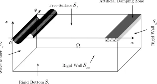
Consider a three-dimensional numerical wave tank with depth

d

, width

B

and length

L

. A layout of the computational domain is illustrated in Figure 1. A wave generator is placed on the upstream wall of the tank. A right-hand Cartesian coordinate system (

Oxyz

) is defined on the mean water surface where the origin is on the corner of the tank, the x-axis is laid on the length of the tank and the positive z-axis directed vertically upwards. An artificial damping zone is defined at adja-cent of the end tank wall.

Figure 1: A definition sketch and coordinates system. x y

z

Wave Maker

w

S

Rigid Bottom

S

_b

Free-Surface

S

_f

Ri

gi

d Wal

ld S Artificial Damping Zone

W

(4)

2.1 Governing equation and boundary conditions

It is assumed that the fluid is homogeneous, incompressible and inviscid and the flow is irrotational and surface tension on the free-surface is neglected. Therefore, velocity potential

f

(

x y z t

, , ,

)

can be introduced. Velocity potential satisfies the Laplace equation in the fluid domain

W

:

2

_f

_{0 in}

 =

W

(1)

There are fully non-linear boundary conditions, Kinematic Free Surface Boundary Condition (KFSBC) and Dynamic Free Surface Boundary Condition (DFSBC) on the free-surface (

S

_f) which can be written as the following (Tanizawa, 2000):

2

(KFSBC)

on

1 (DFSBC)

2

f

t

z

x

y

_S

gz

t

h

f

f h

f

¶

₌

¶

_-

¶ ¶

_-

¶ ¶

¶

¶ ¶

¶

= - - 

¶

(2)

where,

h

(

x y t

, ,

)

is the wave elevation measured from still water level,

t

shows the time of simula-tion and

g

is the gravitational acceleration. Both boundary conditions are satisfied on the exact free-surface.

Impermeable condition is applied on the rigid bottom boundary (

S

_b) and sides and downstream end walls boundaries (

S

_sw,

S

_d) so that,

0 on ,

S

_b

S

_d

and

S

_sw

n

f

¶

=

¶

(3)

where,

n



is the normal vector directed outward of the fluid. Inflow boundary condition can be written as (Tang and Huang, 2008):

on

I

w

S

n

x

f

¶

=

-¶

¶

(4)

where,

f

_I is the theoretical input wave potential. For instantaneous free-surface, the initial condi-tions are defined as:

(

)

(

, ,

, , ,

0

0 )

0

0 on

f

x y t

S

x y z t

h

f

£

=

£

=

(5)

( ) ( )

,

p

( ) ( )

G q p

,

c q

q

G q p

p

d

n

f

G

æ

_¶

ö

_÷

ç

_÷

ç

_÷

=

_ç

-

_÷

G

÷

¶

_÷

çè

ø

ò

(6)

where,

c q

( )

equals zero when the point is outside of the fluid domain and for a point on and inside the boundary domain (

G Î

S

_f



S

_b



S

_d



S

_sw), it is solid angle i.e.,

2 p

for a point on the smooth boundary and

4 p

for a point inside the boundary. For three-dimensional problems,

( )

,

G q p

is given as (Brebbia and Dominguez, 1992):

( )

1 _{( )}

1 ,

,

q p

G q p

r q p

c

=

-



(7)

where,

c



_q and

c



_pare the source and field points location, respectively.

2.2 Desingularized NURBS boundary integral equation

An arbitrary nodal point on the curved free surface can be described by the NURBS as (Piegl and Tiller, 1996)

( )

_{( )}

( )

_{( )}

( )

_{( )}

( )

_{( )}

, 0 0 , 0 0

,

m n l

ij i j i j

i j

m n

l

i j i j

i j

u

v

u v

u

v

k k

v

c

v

= = = =

B

R

= Á

=

B

åå



(8)

where,

R



_{i j}_, and

v

_{i j}_, are control points and weighted function, respectively.

( )

u v

,

Î ê ú

é

_ë

0,1

ù

_û

indicates two directions of the surface, and

m n

,

are the numbers of control points in u and v directions, respectively. k and

l

are the orders of the B-spline basis functions

B

( )_ik

( )

u

and

B

( )_jl

( )

v

which are defined as (Piegl and Tiller, 1996):

( )

_{( )}

( )

_{( )}

( )

_{( )}

( )

_{( )}

0 1

1 ₁ 1

1 1 1

1

0

i i i i i

i i i

i i i i

for u

u

Otherwise

u

k k _k k

k k

+

- _{+ +}

-+

+ + + +

ìï

£ £

ï

B

= í

ïïî

-B

=

B

+

B

-

-(9)

(6)

( )

,

u v u v

u v

n

u v

Á

´Á

=

Á

´Á



(10)

( )

,

u

x y z

u

u v

s

s i

s j

s k

u v

Á

=

+

=

Á



(11)

( )

,

v

x y z

v

u v

t

t i

t j

t k

u v

Á

=

+

=

Á



(12)

where,

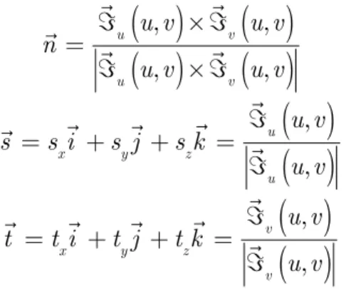
Á



_u and

Á



_vare partial derivatives of NURBS surface in u and v directions shown in Figure 2.

Figure 2: Partial derivatives and unit normal vector.

Location of a nodal (field) point

p

on the surface is expressed as (Piegl and Tiller, 1996)

( )

,

( )

,

0 0

,

m n

p i j i j

i j

u v

c

= =

= Á



=

åå

Â

R



(13) where,

( )

_{( )}

( )

_{( )}

, , 0 0

,

l

ij i j

i j m n

K l

i j i j

i j

u

v

u v

u

v

k

v

= =

B

Â

=

B

åå

(14)

While source point

c



_q is hold outside of

W

and

c



_p on the boundary integration surface. Equation 6 can be written as:

(7)

( ) ( )

,

p

( ) ( )

G q p

,

0 G q p

p

d

n

f

G

æ

_¶

ö

_÷

ç

_÷

ç

_-

_÷

_{G =}

ç

_÷

ç

_¶

_÷

çè

ø

ò

(15)

Equation 15 can be rearranged on the boundaries as (Cao et al. 1991):

( ) ( )

( )

,

N D

N

D

p p

p

G q p

p

d

G q p

d

G q p d

n

G q p

d

n

f

y

j

G G

G

¶

G -

G =

G

¶

-

G

¶

ò



(16)

where,

G

_N represents the boundaries in which the normal flux of potential is known and

G

_D indi-cates boundary in which the known potential is applied, whereas

G Î G

_N



G

_D in which

N

S

b

S

d

S

sw

S

w

G Î



with

f

=

j

and

G Î

_D

S

_f with

¶ ¶ =

f

n

y

.

Since

c



_q and

c



_p are not coincident, integrand singularity is removed. To find the location of

q

c



, the desingularization distance is used which is a function of local grid sizes on the boundary surface as shown in Figure 3. Distance of a source point from the boundary has been proposed as (Cao et al. 1991):

( )

d d m

L

=



D

u

(17)

Figure 3: Distribution of source points and collocation points.

O x

z y

d L

Nodal point Source point

( )

u v,

Á

p

c



u

v

q

(8)

where,

L

_d and u are constant and equal to 1.0 and 0.5, respectively, and

D

_m is the square root of the panel area.

The boundary integral is computed by Gaussian quadrature scheme. Gaussian points are dis-tributed over

( )

u v

,

plane (

_ë

_ê

é

0,1

ù é

_{ú ê}

_{û ë}

´

0,1

ù

_ú

_û

) and field points

c



_p are located on each boundary surface. Thus, the location of the source points cloud can be obtained as:

( ) ( )

( )

,

( ) ( ) ( )

,

( )

,

q p

L p n p

d

u v

d

p

u v

n u v

u v

u

c



=

c



+



= Á



+

 

é

_ê

_ë

L

_ú

_û

ù



= À



(18)

where,



is Gaussian integration weight factor corresponding to Gaussian points and

( )

u v

,

_u _v

L

= Á ´Á



. First term of Equation 16,

G Î

_N

S

_b, can be written as:

( ) ( )

( )

( ) ( )

( )

1 1 0 0

,

1 ,

,

b S p p

G q p

p

d

n

u v n

u v

u v dudv

r

u v

f

¶

G

¶

ì

ü

ï

é

ù é

ù

=

_ê

_ë

Á

_{û ë}

_{ú ê}

Á

_ú

_û

· 

í

_ï

_é

_ù

ý

_ï

L

À

Á

ï

_ê

_ú

ï

ë

û

ï

î

þ

ò

ò ò



_



(19)

Similarly, other Dirichlet boundaries can be evaluated. Suppose that the bottom surface is divided into

M ´ N = M

(

_b

)

segments in u and v directions, respectively. Then, Equation 19 can be written as:

(

)

(

)

(

)

(

)

(

)

,

1 1 1 1

, 1 1

1 ,

,

b b

i j i j p i j i j

I J i j

n m n

m n

u v

n

u v

r

u v

f

M N M N

= = = = M M = =

ì

ü

ï

é

_Á

ù é

_Á

ù

_{· }

_í

_ý

_L

ê

ú ê

ú

ë

û ë

û

ï

_ï

é

_À

_Á

ù

ï

_ï

ê

ú

ï

ë

û

ï

î

þ

=

H

åååå

åå



_







(20)

where,

u

_i and

v

_j

1,..., ,

(

i

=

M =

j

1,...,

N

)

are the Gaussian points located on the bottom sur-face. For the free surface boundary (

G Î

_D

S

_f ), the second integral on the LHS of Equation 16 is discretized as:

(

)

(

)

(

)

{

(

)

}

(

)

,

1 1 1 1

, 1 1

1 ,

,

f b

i j p i j i j i j

I J i j

n m n

m n

n

u v

r

u v

f

d

M N M N

= = = =

M M

= =

é

_Á

ù

_{· }

é

_Á

ù

_L

ê

ú

ê

ú

ë

û

ë

û

é

_À

_Á

ù

(9)

where,

M

and

N

are the number of segments in u and v directions and

d

_n is the normal deriva-tive of potential on the free surface. Other integrals for the remaining boundaries can be discretized similarly.

2.3 Time marching scheme

Material node approach is used to transform Equation 2 from the Eulerian form to the Lagrangian form. Nodal points are allowed to freely move with the particles of free surface. Then, Equation 2 can be written as (Tanizawa, 2000):

2

1

2 _on

f

g

t

_S

t

df

_h

_f

d

dc

_f

d

= -

+ 

= 



(22)

where,

c



is the location of particles on the free-surface. The position of the particles is updated by the evaluation of particle velocity on the free-surface and Fourth-order Runge-Kutta time integra-tion approach.

2.4 Tangential derivatives

Since, geometry of the free-surface is described by NURBS, the normal and tangential unit vector components are provided by Equations 10, 11 and 12. The potential variation on the free-surface can also be described by NURBS as:

( )

,

( )

,

0 0

,

m n

i j i j

i j

u v

f

= =

= Ã

=

åå

Â

Q

₍₂₃₎

where,

Q

_{i j}_, is potential on the control points and evaluated by potential of nodal points which do not participate in the basis function. Directional derivatives of

f

with respect to u and v can be written as (Piegl and Tiller, 1996):

( )

_{( )}

( )

_{( )}

, 0 0

,

l

m n

ij i j

u m n i j

K l

i j

i j i j

i j

u

v

u v

u

v

k

v

f

v

= =

¢

B

¶

= Ã

=

Q

¶

_¢

B

åå

(24)

( )

_{( )}

( )

_{( )}

, 0 0

,

l

m n

ij j i

v m n i j

l i j

i j j i

i j

v

u

u v

v

u

k

v

f

v

= =

¢

B

¶

= Ã

=

Q

¶

_¢

B

åå

(25)

(10)

( )

,

1 ,

u s

u

u v

s

u

u v

f

=

¶

=

¶

=

Ã

¶



¶

_Á



(26)

( )

,

1 ,

v t

v

u v

t

v

u v

f

=

¶

=

¶

=

Ã

¶



¶

_Á



(27)

The particle velocity represented on the boundary can be represented by

 =

f

_s

s



+

f

_t

t



+

f

_n

n



in which

f

_n is the normal derivative of potential.

2.5 Artificial wave generator

Extreme waves described by linear and second-order Stokes wave theories are imposed on the inflow boundary. These are written as follows:

( )1 ( )2

I I I

f

=

f

+

f

(28)

and also,

( )1 ( )2

I I I

h

=

h

+

h

(29)

where,

f

_I( )1 and

h

_I( )1 correspond to first-order potential and wave profile, respectively, and

f

_I( )2 and ( )2

I

h

correspond to the second-order Stokes wave properties (Ning et al., 2009). A ramping function is engaged to avoid the impulse-like behavior and keep the stability of solutions and to reach to the steady state properly. In the present modeling, the ramping function given by Tang and Huang (2008) is used:

( )

2

1

1 cos

,

1 ,

m

m m

m

t

T

f

t

T

t

T

p

ì æ

ö

ï

_÷

ï ç

_÷

ï ç -

_÷

£

ï ç

_÷÷

=

_{í è}

ç

_ø

ïï

_>

ïïî

(30)

where,

T

_m is the modulation time which equals to the incident wave period in the present study.

2.6 Artificial damping zones

(11)

( )(

)

(

) ( )(

)

on

1 .

2

e

f

e

x

t

_S

g

x

t

dc

_{f n}

_{c c}

d

df

h

f f

n

f f

d

=  -

-= - +

  -

-

_

(31)

where, the subscript ecorresponds to the reference configuration for the fluid. The function

n

( )

x

is damping coefficient defined by

( )

(

0

)

2 0 1 0

2 ,

2 k

x

k

pb

n

aw

p

é

ù

ê

ú

=

_ê

-

_ú

£ £

=

+

ë

û

(32)

in which, w is a characteristic wave frequency and

k

is a characteristic wave number. The param-eters a and

b

control the strength and extent of the damping zone, respectively.

x

₀ and

x

₁ indi-cate the edges of the damping zones in horizontal plane on the free-surface. The terms

f

_e and

c



_e are reference values. When reference values are set for calm water condition (

f

_e

=

0 ,

h

=

0

), damping zone acts as simple absorber. If a propagating wave is used as reference value, then the damping zone allows only this wave to pass through. In practice, the damping coefficient equals zero except in the damping zone

(

x

₀

£ £

x

₁

)

, which is continuous and continuously differentia-ble.

3 NUMERICAL RESULTS

3.1 Convergence test and model verification

To perform the numerical simulation, a numerical wave tank of Ning and Teng (2006) is provided. The dimension of the wave tank is taken as

15.45 m

length,

0.3 m

width and

0.8 m

depth. Linear wave with the wavelength of

l

=

5.15 m

and wave slope of

kA

=

0.033

is specified for inflow boundary value. An artificial damping zone is extended along a wave length foreside of end wall tank. A numerical wave probe is adopted at

(

0.28 , 0.5

L

B

)

in horizontal plane. The solution of proposed NURBS NWT for

4 24

´

nodal points in u and v directions respectively, time step

40

(12)

Latin American Journal of Solids and Structures 11 (2014) 2308-2332 Figure 4: Comparison of analytical and numerical modeling of linear wave, h A vs. dimensionless time.

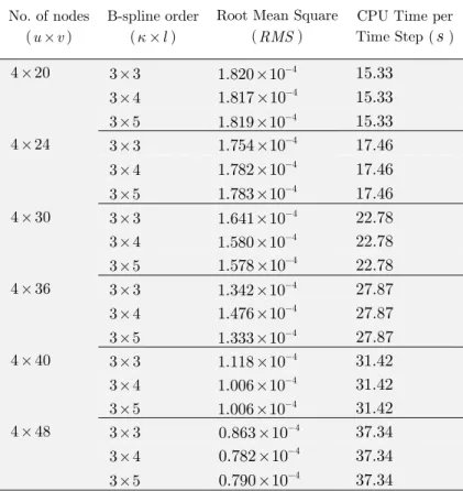
When the wave is fully developed, analytical solution and numerical computations with different number of nodal points are tabulated on Table 1. Root mean square of wave elevation for a com-plete wave period at the raised numerical probe is defined as:

2 .

1

K _iExact _iNum Exact i i

RMS

K

h

=

ì

ü

ï

-

ï

=

í

_ï

ý

_ï

ï

î

þ

å

(33)

where,

K

is the number of the time steps to complete a wave period with time step

T

40

. NURBS NWT is run with a desktop PC (Intel Core 2 Quad CPU, 2.66 GHz, and 2 GB of RAM). It is shown that to achieve about half of RMS corresponds to

4 20

´

nodal points, more than twice CPU time is taken for

4 ´

48

nodal points at each time step.

Accuracy of the present model for different wave slopes and wave frequencies of second-order stokes wave is examined and given in Table 2. Hence, three wave slopes are chosen and RMS of wave ele-vations is determined for

4 ´

30

nodal points on free surface and time step

T

40

. The order of B-spline basis function is chosen

k

´ = ´

l

3 3

. It is shown that increasing wave slope decreases the accuracy of solution. For

kA

=

0.104

, the wave slope is greater than

kA

=

0.033

about three time but, increasing of RMS is infinitesimal.

Effect of time step on the numerical solution is given in Figure 5. In this Figure the solutions of input second-order stokes wave with

kA

=

0.104

and different time step with water depth 0.5 is compared. Mesh size and order of B-spline basis function is the same as for Table 2. For time step

90 T

, fully development of the input wave is postponed due to the coarse time steps. For

10 t T



, the wave is fully developed for three time steps and the numerical solutions are inde-pendent from the time step.

* **

*

**

*

**

*

**

*

t/T





0 5 10 15 20

(13)

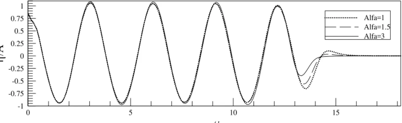
To obtain the proper solution of NWTs, the damping zones should be adopted. A part of wave en-ergy will return back to the computational domain from downstream boundary if the damping of wave energy is too weak. On the other hand, if the absorbing strength is too powerful, the damping zone will act as a solid boundary and the waves reflect from outflow boundary. The length and strength of damping zone control the performance of damping zone. Therefore, for different parame-ters a and

b

the wave elevation of free surface is compared in Figure 6 and Figure 7, respectively. In Figure 6, the free surface oscillations along the numerical tank (

x d

) due to the input second-order stokes wave for

b

=

2

and different a are shown. When the strength of the damping zone is increased the damping zone acts as the rigid walls and some portion of incident wave is reflected. For

a

=

3

, increment of the wave height is happen due to wave reflection. For

a

=

1

and

1.5 a

=

, the wave reflection is reduced from the wave absorber.

For different length of the damping zone, the wave elevation for

a

=

1

is given along the numeri-cal wave tank in Figure 7. For

b

=

1

, the wave absorber do not dissipate the incident wave and for long simulation the wave reflection is happened severely. For

b

=

2

and

b

=

3

, the incident wave is fully dissipated within the wave absorber and open water condition is kept.

3.2 Focused wave generation and propagation

In the experimental work, data measurement of non-linear waves is transformed in the Fourier do-main as presented by Ning et al. (2009) and wave spectrum

S f

( )

is manifested. Indeed, it repre-sents wave components with different amplitudes and periods which interact with each other and consequently make extreme wave. Amplitude of each wave component

a

_i is obtained as:

( )

i i

i n

S f

f

a

A

S f

f

D

=

D

å

(34)

where,

A

is the general linear focused wave amplitude given by Ning et al. (2009),

S f

_i

( )

is the spectral density of each wave component

i

and

D

f

is the frequency step depending upon the number of wave components

n

.

For a wave flume with water depth of

d

=

0.5 m

, spectrums are presented in Figure 8. Char-acters of each wave spectrum are depicted in Table 3 based on Westphalen et al. (2012) in order to simulate the wave in which

T

_p is the peak period of wave spectrum and

l

_p is the wave length corresponding to the peak period.

In this paper, an artificial wave generator is located at

x

=

0

and an artificial damping zone with the length twice as great as the length of the wave is placed at the end of the tank. To verify proposed numerical procedure, a tank with the dimensions of

12 m

´

1 m

´

0.5 m

(

L

´ ´

B

d

) is provided and the focused point and time are set to

x

₀

=

3 m

and

t

₀

=

9.2 s

for case 2,

0

3.27

(14)

basis function of order

3 3

´

is used to simulate the free-surface elevation. Other boundaries are flat and described by isoperimetric linear quadrilateral elements. Time step

D =

t

T

_p

40

is used in high-order time integration scheme.

Figure 5: Comparison of numerical modeling of linear wave for different time steps, h A vs. dimensionless time.

Figure 6: Performance of the end wall damping zone for different strength of the damping zone.

Figure 7: Performance of the end wall damping zone for different length of the damping zone. t/T





0 5 10 15 20

-1 -0.5 0 0.5 1

dt=T/30 dt=T/60 dt=T/90

x/d





0 5 10 15

-1 -0.75 -0.5 -0.25 0 0.25 0.5 0.75 1

Alfa=1 Alfa=1.5 Alfa=3

x/d





0 5 10 15

-1 -0.5 0 0.5

1 _Beta=1

(15)

Latin American Journal of Solids and Structures 11 (2014) 2308-2332 No. of nodes

(u´v)

B-spline order (k´l)

Root Mean Square (RMS)

CPU Time per Time Step (s)

4´20 3 3´ _{1.820 10}_´ -4 _15.33

3 4´ _{1.817 10}_´ -4 _15.33

3 5´ _{1.819 10}_´ -4 _15.33

4´24 3 3´ 1.754 10´ -4 17.46

3 4´ 1.782 10´ -4 17.46

3 5´ 1.783 10´ -4 17.46

4´30 3 3´ _{1.641 10}_´ -4 _22.78

3 4´ _{1.580 10}_´ -4 _22.78

3 5´ 1.578 10´ -4 22.78

4´36 3 3´ _{1.342 10}_´ -4 _27.87

3 4´ 1.476 10´ -4 27.87

3 5´ _{1.333 10}_´ -4 _27.87

4´40 3 3´ _{1.118 10}_´ -4 _31.42

3 4´ _{1.006 10}_´ -4 _31.42

3 5´ _{1.006 10}_´ -4 _31.42

4´48 3 3´ _{0.863 10}_´ -4 _37.34

3 4´ _{0.782 10}_´ -4 _37.34

3 5´ _{0.790 10}_´ -4 _37.34

Table 1: RMS error and CPU time of linear wave simulation.

Wave slope Wave celerity Root Mean Square

(kA) (C =w k) (RMS)

0.015 2.7146 _{9.971 10}_´ -5

0.033 2.4580 _{1.641 10}_´ -4

0.104 1.5924 _{1.809 10}_´ -4

Table 2: RMS error and CPU time of linear wave simulation.

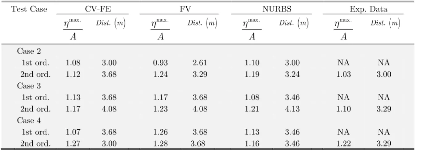
The maximum linear and nonlinear wave elevations _hmax._{for the cases given in Table 3 are}

(16)

Latin American Journal of Solids and Structures 11 (2014) 2308-2332 Figure 8: Wave spectrum of focused wave and properties of simulated cases.

Test Case frange(Hz) n A m ( ) Tp ( )s lp ( )m

Case 2 0.6-1.3 16 0.0632 1.2 2.00

Case 3 0.6-1.4 20 0.0875 1.25 2.18

Case 4 0.5-1.8 16 0.1020 1.25 2.18

Table 3: Properties of wave cases for simulation.

For case 2, the highest crest of the first-order wave input with NURBS NWT is higher than the evaluations with CV-FE and FV solver. For the second-order wave components, NURBS NWT predicts the maximum wave elevation closer to the experimental measurement than the FV solver.

f (Hz)

S(

f)

0 0.5 1 1.5 2 2.5 3 3.5 4

0 1 2 3 4 5 6 7 8 9 10

Case 2

f (Hz)

S(

f)

0 0.5 1 1.5 2 2.5 3 3.5 4

0 1 2 3 4 5 6 7 8 9 10

Case 3

f (Hz)

S(

f)

0 0.5 1 1.5 2 2.5 3 3.5 4

0 1 2 3 4 5 6 7 8 9 10

(17)

For case 3, the trend is similar. For case 4, the numerical results show good agreements with the experimental data. It should be mentioned that in this case, the focused wave almost broke in the real wave tank and the nonlinearity predominates on the simulation.

Test Case CV-FE FV NURBS Exp. Data

max.

A

h Dist.

( )

m max.

A

h Dist.

( )

m max.

A

h Dist.

( )

m max.

A

h Dist.

( )

m

Case 2

1st ord. 1.08 3.00 0.93 2.61 1.10 3.00 NA NA

2nd ord. 1.12 3.68 1.24 3.29 1.19 3.24 1.03 3.00

Case 3

1st ord. 1.13 3.68 1.17 3.68 1.08 3.46 NA NA

2nd ord. 1.17 4.08 1.23 4.08 1.21 4.13 1.10 3.29

Case 4

1st ord. 1.07 3.68 1.26 3.68 1.13 3.46 NA NA

2nd ord. 1.27 3.00 1.28 3.68 1.16 3.46 1.22 3.29

Table 4: Maximum wave elevation of three focused wave.

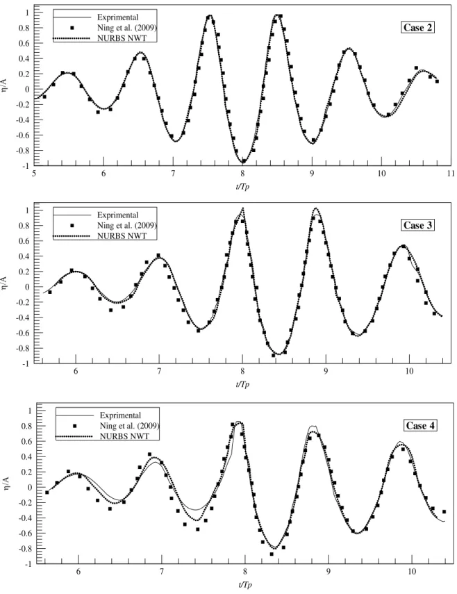
Time series of wave elevations of the cases 2-4 are depicted at focused point in Figure 9 and Fig-ure 10, respectively. The comparison of computed crest and trough focused waves using linear and nonlinear theory with experimental results is presented. For case2, computational wave crest on the center of wave group is reached to the experimental measurement by NURBS NWT. When the input wave includes the second-order wave components, prediction of the central wave group trough coincides with physical wave tank measurement as shown in Figure 10. The results of the surround-ing crests and troughs are generally improved from the first-order to the second-order. For both input wave cases, the surrounding trough elevations are slightly higher than the physical experi-ments with respect to the surrounding crests and somewhat, NURBS NWT decreases the small differences.

For case 3, it can be said that the numerical evaluations are closer to the physical experiments bet-ter than case 2 and the slight difference of the surrounding troughs and crests are decreased. It shows that moving from input linear wave components to the second-order wave components im-proves trough elevations.

(18)

Latin American Journal of Solids and Structures 11 (2014) 2308-2332 Figure 9: Comparison of time history of wave elevation of the first-order focused wave cases 2-4.

t/Tp





6 7 8 9 10

-1 -0.8 -0.6 -0.4 -0.2 0 0.2 0.4 0.6 0.8 1

Exprimental Ning et al. (2009) NURBS NWT

Case 2

t/Tp





6 7 8 9 10

-0.8 -0.6 -0.4 -0.2 0 0.2 0.4 0.6 0.8 1 1.2

Case 3

t/Tp





6 7 8 9 10

-0.8 -0.6 -0.4 -0.2 0 0.2 0.4 0.6 0.8 1

1.2 _Exprimental

Ning et al. (2009) NURBS NWT

(19)

Figure 10: Comparison of time history of wave elevation of the second-order focused wave cases 2-4. t/Tp





5 6 7 8 9 10 11

-1 -0.8 -0.6 -0.4 -0.2 0 0.2 0.4 0.6 0.8 1

Case 2

t/Tp





6 7 8 9 10

-1 -0.8 -0.6 -0.4 -0.2 0 0.2 0.4 0.6 0.8

1 _Exprimental

Ning et al. (2009) NURBS NWT

Case 3

t/Tp





6 7 8 9 10

-1 -0.8 -0.6 -0.4 -0.2 0 0.2 0.4 0.6 0.8 1

(20)

Experimental investigation on propagation of incident irregular waves over a submerged bar is car-ried out by Beji and Battjes (1993) and its numerical simulations based on Boussinesq equations and mild-slope equations are conducted by Hsu et al. (2007) and (2002), respectively. JONSWAP spectrum of Hsu et al. (2007) given in Equation 35 is chosen to pass over a submerged bar. Dimen-sions of numerical wave tank is equal to the experimental wave flume of Beji and Battjes (1993) with the length of

37.7 m

, the breadth of

0.8 m

and the water depth of

0.4 m

.

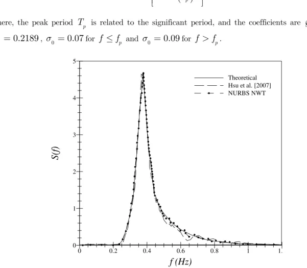
Spectrum of the fully propagated incident wave with significant wave height of

H

_{1 3}

=

0.03 m

and the significant period of

T

_s

=

2.5 s

is compared with the theoretical result and numerical computation in Figure 11.

( )

(

)

2 2 0 4 _exp ₁ ₂ 2

2 5

1 1 3

exp

1.25

p

f f

p

f

S f

f H

f

s

é _æ _ö ù

ê ç ÷_÷ ú

- _{ê è}êê-ççç_ç -÷÷÷_÷_ø úú_ú

- êë úû

é

_{æ ö}

ù

ê

_{ç ÷}

_ç

÷

ú

ê

ú

=

_ê

-

_{ç ÷}

÷

_ú

Ã

çè ø

ê

ú

ë

û

(35)

where, the peak period

T

_p is related to the significant period, and the coefficients are

Ã =

3.3

, 1

0.2189

s

=

,

s

₀

=

0.07

for

f

£

f

_p and

s

₀

=

0.09

for

f

>

f

_p.

Figure 11: Comparison of JONSWAP spectrum recorded in physical and numerical wave tank.

It seems that there are trivial mismatch at the peak spectrum in Hsu et al. (2007) computations which is improved by the present model. Furthermore, the deviation between theoretical and

nu-f (Hz)

S(f

)

0 0.2 0.4 0.6 0.8 1 1.

0 1 2 3 4 5

(21)

merical results is remained on the higher frequency domain, but it seems that NURBS NWT model is closer to the proposed spectrum. To measure the irregular wave evolution due to a submerged trapezoidal bar, eight wave probes are arranged along the wave flume as shown in Figure 12.

It is worth mentioning that the wave breaking does not occur during the simulation and the observation is conducted at the first wave probe. Comparison of the experiments and the numerical results is given in Figure 13. At the peak point of energy density at every wave probes, NURBS NWT is better than the other numerical computations, whereas the mild slop simulation for wave probes 5-8 and the Boussinesq simulation for wave probe 2 and 4 are overestimated. In addition, these simulations do not touch peak measurement at wave probes 1 and 3. For higher frequency, substantial deviation occurs at wave probes 5-8 for numerical simulation showing that computations are partly improved by NURBS NWT.

Figure 12: Wave probe arrangement along the wave flume of Beji and Battjes (1993).

4 CONCLUSIONS

Development of a fully non-linear 3D NWT is considered in this paper for investigation of propaga-tion and scattering of non-linear random sea wave due to bottom submerged bars. The simulapropaga-tion of fully non-linear waves using NURBS in a potential three-dimensional numerical wave tank is successfully completed.

MEL method and desingularized boundary element method is employed for numerical simula-tion. To keep numerical accuracy and avoid instability in MEL, five points Chebyshev smoothing scheme was adopted in time marching. To obtain appropriate numerical solutions for wave propa-gation problem in a numerical wave tank artificial damping zones (sponger layer) is adopted. Per-turbation sources are placed on the fixed inflow boundary to make the free-surface oscillating during the simulation. Also, the NURBS is used to evaluate velocity of the free surface particles accurately. It is a novel procedure to calculate the free-surface kinematics.

The stability and accuracy of NURBS NWT were examined and verified to model the free-surface. It is shown that the present approach gives accurate solution, whereas the computation time was saved and the computational nodes were reduced. Simulations of propagation of irregular

2.0m 3.0m 1:10 1:20

o

x

Propagation Direction z

0.3m

6.0m 6.0m 18.75m

0.4m

1.95m 5.0m

1m

1m 1m1m 1m1m

(22)

wave spectrum and wave transformation of a random sea waves due to submerged bar are present-ed and comparpresent-ed with the experimental and available numerical results. It is shown that the appro-priate solution with sufficient accuracy can be obtained by the proposed numerical procedure.

f (Hz)

S(

f)

[c

m

.cm

/H

z]

0 0.5 1 1.5 2

Beji and Battjes [1993] Hsu et al. [2002] Hsu et al. [2007] NURBS NWT

Wave Probe 1

f (Hz)

S(f

)

[c

m.c

m

/H

z]

0 0.5 1 1.5 2

Wave Probe 2

f (Hz)

S

(f

)

[c

m

.c

m

/H

z]

0 0.5 1 1.5 2

Wave Probe 3

f (Hz)

S(

f)

[c

m

.cm

/H

z]

0 0.5 1 1.5 2

(23)

Figure 10: Comparison of irregular wave transformation when propagating over the submerged bar.

References

Abbasnia, A., Ghiasi, M. (2014). Nonlinear wave transmission and pressure on the fixed truncated breakwater using NURBS numerical wave tank, Latin American Journal of solids and structures 11(1): 51-74.

Beji, S., Battijes, J.A. (1993). Experimental investigation of wave propagation over a bar, Journal of Coastal Engi-neering 19: 151-162.

Brebbia, C.A., Dominguez, I. (1992). Boundary elements: An introductory course, WIT Press.

Cabral, J.J.S.P, Wrobel, L.C. and Brebbia C.A. (1990). A BEM formulation using B-splines: I- uniform blending functions, Engineering Analysis with Boundary Elements 7: 136-144.

f (Hz)

S(f

)

[c

m.c

m

/H

z]

0 0.5 1 1.5 2

Wave Probe 5

f (Hz)

S(f

)

[c

m.c

m

/H

z]

0 0.5 1 1.5 2

Wave Probe 6

f (Hz)

S(f

)

[c

m.c

m

/H

z]

0 0.5 1 1.5 2

Wave Probe 7

f (Hz)

S(f

)

[c

m.c

m

/H

z]

0 0.5 1 1.5 2

(24)

Latin American Journal of Solids and Structures 11 (2014) 2308-2332 Cabral, J.J.S.P, Wrobel, L.C. and Brebbia C.A. (1991). A BEM formulation using B-splines: I- multiple knots and non-uniform blending functions, Engineering Analysis with Boundary Elements 8: 51-55.

Cao, Y., Schultz, W.W., Beck, R.F. (1991). Three-dimensional desingularized boundary integral method for potential problems, International Journal of Numerical Methods in Fluids 12: 758-803.

Cointe, R. (1991). Free surface flows close to a surface piercing body, Mathematical Approaches in Hydrodynamics 319-334.

Damanpack, A.R., Bodaghi, M., Ghassemi, H., Sayehbani, M. (2013). Boundary element method applied to the bending analysis of thin functionally graded plates, Latin American Journal of Solids and Structures 10(3): 549-570. Datta, R., Sen, D. (2006). A B-spline solver for the forward-speed diffraction problem of a floating body in the time domain, Applied Ocean Research 28: 147-160.

Gao, Z.L., Zou, Z.J. (2008). A three-dimensional desingularized high order panel method based on NURBS, Journal of Hydrodynamics 20(2): 137-146.

Grilli, S.T., Guyenne, P., Dias, F. (2001). A fully non-linear three-dimensional overturning waves over arbitrary bottom, International Journal of Numerical Methods in Fluids 35: 829-869.

Grilli, S.T., Svendsen, I.A. (1990). Corner problems and global accuracy in the boundary element solution of nonlin-ear wave flow, Journal of Engineering Analysis with Boundary Elements 7: 178-195.

Hsu, T.W., Hisiao, S.C., Ou, S.H., Wang, S.K., Yang, B.D., Chou, S.E. (2007). An application of Boussinesq equa-tions to Bragg reflection of irregular waves. Ocean Engineering 34: 870-883.

Hsu, T.W., Liao, J.M., Teng, C.H., Hsieh, W.B. (2002). Simulating wave transformations of irregular waves by mild-slope equation, In Proceedings of the 24th Ocean Engineering Conference, Taiwan 70-77.

Koo, W. (2003). Fully nonlinear wave-body interaction by a 2D potential numerical wave tank. PhD Thesis, Texas A&M University, Austin, United State of America.

Koo, W., Kim, M.H. (2004). Nonlinear wave-floating body interactions by a 2D fully nonlinear numerical wave tank, In Proceeding 14th International Offshore and Polar Engineering Conference, Toulon, France 23-28.

Li M., Zhang, H., Guan, H. (2011). Study of offshore monopile behaviour due to ocean waves, Ocean Engineering 38: 1946-1956.

Longuet-Higgins, M.S., Cokelet, E.D. (1976). The deformation of steep surface waves on water (Ι) - a numerical method of computation, In Proceeding of The Royal Society of London, London, England 1-26.

Newman, J.N. (2010). Analysis of wave generators and absorbers in basins, Journal of Applied Ocean Research, 32: 71-82.

Ning, D.Z., Teng, B. (2006). Numerical simulation of fully nonlinear irregular wave tank in three-dimension, Interna-tional Journal of Numererical Methods in Fluids 53: 1847-1862.

Ning, D.Z., Zang, J., Liu, S.X., Eatock Taylor, R., Teng; B., Taylaor P.H. (2009). Free-surface evolution and wave kinematics for nonlinear uni-directional focused wave groups, Ocean Engineering 36: 1226-1243.

Piegl, L.A., Tiller, w. (1996). NURBS book. Springer, New York.

Shao, Y.L. (2010). Numerical potential-flow studies on weakly-nonlinear wave-body interaction with/without small forward speeds. PhD Thesis, NTNU, Norway.

Tanizawa, K. (2000). The state of the art on numerical wave tank, In Proceeding of 4th Osaka Colloquium on Sea-keeping Performance of Ships, Japan 95-114.

Tang, H.J., Huang, C.C. (2008). Bragg reflection in a fully nonlinear numerical wave tank based on boundary inte-gral equation method. Ocean Engineering 35: 1800-1810.

(25)

Wu, N.J., Tsay, T.K., Young D.l. (2005). Meshless numerical simulation for fully nonlinear water waves, Interna-tional Journal of Numerical Methods in Fluids 50: 219-234.

Xiao, L.F., Yang, J.M., Peng, T., Li, J. (2009). A meshless numerical wave tank for simulation of nonlinear irregular waves in shallow Water, International Journal of Numerical Methods in Fluids 61: 165-184.