Scattering of Fexural Gravity Waves by a Two-Dimensional Thin Plate

J_{ournal of} A_pplied F_luid M_{echanics, Vol. 10, No. 1, pp. 199-208, 2017.} Available online at www.jafmonline.net, ISSN 1735-3572, EISSN 1735-3645.

Scattering of Fexural Gravity Waves by a

Two-Dimensional Thin Plate

S. Banerjea

1†

, P. Maiti

2

and D. Mondal

3

1 _{Department of Mathematics, Jadavpur University, Kolkata-700032, India}

2 _{Four year B. Tech. Course, Technology Campus, Calcutta University , JB 2, Sector III, Kolkata 700098,}

India

3 _{Government General Degree College at Kalna-1, Muragacha, Medgachi, Burdwan-713405, India.}

†Corresponding Author Email: sudeshna.banerjea@yahoo.co.in (Received July 22, 2015; accepted February 1, 2016)

A

BSTRACT

An approximate analysis based on standard perturbation technique together with an application of Green’s integral theorem is used in this paper to study the problem of scattering of water waves by a two dimensional thin plate submerged in deep ocean with ice cover. The reflection and transmission coefficients upto first order are obtained in terms of the shape function describing the plate and are studied graphically for different shapes of the plate.

Keywords: Water wave scattering; Two dimensional thin plate; Nearly vertical plate; Reflection coefficient; Transmission coefficient.

1.

I

NTRODUCTION

The study of ocean wave interactions with a thin,

floating elastic plate has gained immense importance since last decade as it can be used to model a wide range of physical systems. One of its important applications consists in modelling a very large floating structure (VLFS), that is used in ocean space utilization for the construction of megafloats such as floating airports, offsh ore runways, floating restaurant etc. It is a technology that allows these megafloats, which are considered to be artificial lands to float on rising sea level and has a minimal effect on marine habitat, natural and tidal current

flow (cf Wang et al. 2010; Wadhams 1978). Owing to the large surface area and relatively small depth, VLFS behaves elastically under wave action (cf Wang et al. 2010). In the polar region, surface gravity waves propagate from the open ocean into ice-covered seas. Understanding the modus operandi of formation of sea ice and its distribution is imperative to explain the geophysical phenomena occurring in the polar regions and in the marginal ice zone. A precinct between ocean and atmosphere, the sea ice arrests the escape of heat from the ocean to the air above. Consequently it plays a crucial role in conservation of marine life. An uninterrupted expanse of unbroken ice over a vast stretch in the polar region often encounters waves propagating at free surface. It is well known that waves may

weaken and rupture the continuous sea ice causing

important. Mathematically, the boundary value problem (BVP) related to study of water waves in ocean with ice-cover, involves fifth order derivative of the potential function in the boundary condition on ice cover whereas the governing partial differential equation is of second order. The literature concerning the study of ocean wave interaction in ocean with ice-cover in the presence of a body submerged beneath the ice-cover floating in a deep water is rather limited, although the study of ocean wave interaction with structures present in the ocean with free surface under linearised theory has been a subject of interest since early twentieth century. A number of researchers contributed significantly to this topic, although the closed form solution to these problems are available only when the structure is in form of a thin rigid vertical plate and that too for the two dimensional motion in water. Diffraction problems involving nearly vertical barriers are more general than vertical barrier. One such problem of water waves scattering by a nearly vertical plate partially immersed in deep water was considered by Shaw (1985). He used a perturbation analysis that involved solution of singular integral equation. Later Mandal and Chakrabarti (1989) and Mandal and Kundu (1990) considered the problems of water waves scattering by a nearly vertical barrier and utilized a perturbation analysis different from Shaw (1985) to handle the problems. The problem of water wave diffraction by a symmetric two dimensional thin slender was plate mentioned briefly by Shaw (1985) although the first order correction to reflection and transmission coefficients are not given there explicitly. Later Kundu (1997), Kundu and Saha (1998) considered the problem of water wave scattering by a thin two dimensional slender body either partially immersed or completely submerged or submerged in deep water. They used the perturbation technique described in Mandal and Chakrabarti (1989) to obtain first order correction to reflection and transmission coefficients in terms of the shape functions of two sides of the slender barrier. All the above mentioned wave structure interaction problems were considered when the water region is covered by a free surface. In recent past Das and Mandal (2007) investigated the problem of ocean water and sea ice interaction in presence of a long horizontal cylinder. Maiti and Mandal (2010), Maiti et al. (2011) studied the ocean wave interaction with a thin vertical barrier present in ocean with ice cover. They used Green’s integral theorem to reduce the corresponding boundary value problem to a hyper-singuler integral equation which was then solved by collocation method. In the present paper we have studied the problem of scattering of ocean waves by two dimensional thin plate submerged in ocean with ice cover. Using the perturbation analysis as given by Mandal and Chakrabarti (1989), together with application of Green’s integral theorem, the first order correction to the reflection and transmission coefficient are obtained in terms of the shape function describing the shape of two sides of the plate, which are then studied graphically for various values of wave number and different values of ice cover parameter. The reflection and transmission coefficients up to

first order due to the two dimensional thin barrier are compared with those due to one dimensional nearly vertical barrier submerged in ocean with ice-cover. It was also observed that when the value of ice-cover parameters are small, the reflection and transmission coefficients matches with the results in 1998 when the ocean is covered by a free surface. It is observed that unlike nearly vertical plate, the thickness of the symmetric two dimensional plate has some effect on the reflection and transmission coefficient. From the graph it is noted that in presence of a symmetric two dimensional plate, the long waves do not feel the presence of ice-cover as they are confined towards the bottom of the ocean. However, the short waves which are confined near the ice-cover surface are affected by the presence of ice-cover. It is observed that long plate induces more reflection of wave energy and less transmission. Also for a particular length of the plate, the increase in ice cover parameter induces more transmission of wave energy.

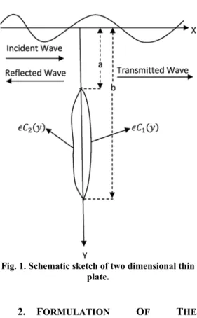
Fig. 1. Schematic sketch of two dimensional thin plate.

2.

F

ORMULATION

O

F

T

HE

P

ROBLEM

We consider two dimensional irrotational motion in ocean with ice cover due to scattering of time harmonic incident wave by a two dimensional thin barrier submerged in infinitely deep ocean. We choose a rectangular cartesian coordinate system in which y axis is vertically downwards into fluid region y ≥ 0 and x axis is along rest position of lower part of ice-cover. Ice-cover is modelled as a thin elastic plate of thickness h₁ and density ₁ with

flexural rigidity

3 1 2

12(1 ) Eh L

 

Young’s modulus, is the Poisson ratio of the elastic material of the ice-cover. A thin two dimensional rigid plate described by S S₁ S₂ where S₁ and

2

S denote two sides of two dimensional thin plate given respectively by x C y₁( ) and

2( ),

x C y a y b (cf figure 1).

Here is a non dimensional small parameter which can be regarded as a measure of thinness of the plate and C yi( ) , i1, 2 are bounded continuous function of y with C ai( )C bi( )0,i1,2.. A train of time harmonic waves represented by velocity potential Re



inc( , )x y ei t



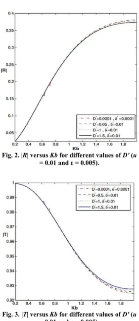
where σ is the circular frequency, is incident upon the barrier from negative infinity and is partially reflected by the barrier and partially transmitted over and below the barrier.

Fig. 2. |R_{| versus} Kb _{for different values of} D′₍u

= 0.01 and = 0.005).

Fig. 3. |T_{| versus} Kb _{for different values of} D′₍u

= 0.01 and = 0.005).

Assuming linearised theory, the motion is described by the velocity potential Re



( , )x y ei t



where φ

satisfies,

2

0, y 0, 

   (1) the linearised ice cover condition (cf Landau and Lipschitz (1970) pp 44),

4 4

(D K 1) _y K 0 on y=0,

x   

 _{   }



(2)

the condition on the barrier,

1

2

( , ) 0 on ( ),

( , ) 0 on ( ) ,

x y x C y a y b

n

x y x C y a y b

n

 _

 _

 _{   }



 _{   }



(3)

where n 

 denotes the normal derivative to the barrier,

the edge condition,

1 2

r is bounded as r0, (4) the bottom condition

0 as y 

    (5) Also ϕ(x,y) satisfies the far field conditions given by

( , ) ( , ) as , ( , )~

( , ) as .

inc inc

inc

x y R x y x

x y

T x y x

 





 _{   }

 

 

 (6)

Here R and T are the reflection and transmission coefficients. Also,

( , ) ,

inc _{x y e} Ky i Kx

    (7) where k = λK is the unique positive root of the dispersion relation



4



1 0,

Dk  K kK (8)

Here

2

,

K g

g 

  acceleration due to gravity,

, L ρg

L

D is the flexural rigidity of ice-cover as mentioned before, ρ is the density of fluid and

1 1.

h  



 .

The other roots of (2) are ₁K, , ₁K ₂Kand 2K

with Re

 

₁ > 0 and Re

 

₂ < 0. A detailed discussion on the roots of dispersion relation (2)is given in Chakrabarti et al. (2003).









1 ( 0, )

2 ( 0, )

( ) ( 0, ) , ( , )

( ) ( 0, ) . y y y y d

C y y

x dy

a y b

x y

d

C y y

x dy

a y b

 _   _    _{ }     _{ }  _  _{ }       

 (9)

3.

M

ETHOD

O

F

S

OLUTION

The form of the approximate boundary condition given by (9) suggest that we may expand the function

( , )x y

 and the two unknown physical constant R and T in terms of the small parameter as

0 1 ^

( , )x y ( , )x y ( , )x y o( 2),











 (10)

2

0 1 ( ),

RR  Ro (11)

2

0 1 ( ).

TT  T o (12) Substituting  , R, T from (10), (11), (12) into (1),(2), (5) to (7) and equating the coefficients of 0 and 1 from both sides of the equations we find that

0

 and ₁ satisfies the following two boundary value problems(BVPs).

BVP − 0: The function ₀ satisfies

2

0 0, y 0,



   (13)

4

0 0

4

(D K 1) _y K 0 on y 0,

x  

 _{    }

 (14)

0x 0, on x 0, a y b,

     (15)

1 2

0 is bounded as 0,

r  r (16)

0 0 as y , 

    (17)

0 0

0

( , ) ( , ) as ( , )~

( , ) as .

inc inc

inc

x y R x y x

x y

T x y x

     _{   }      (18)

BVP − 1: The function ₁ satisfies

2

1 0, y 0,



   (19)

4

1 1

4

(D K 1) _y K 0 on y 0,

x  

 _{    }

 (20)

1

1 0

( 0, )

{ ( ) _y( 0, )} , y

d

C y y a y b

x dy  _        1 2 0

( 0, )

{ ( ) _y( 0, )} y

d

C y y a y b

x dy

 _

 

   

 (21)

1 2

1 is bounded as 0,

r  r (22)

1 0 as y , 

    (23)

1 1

1

( , ) as , ( , )~

( , ) as . inc

inc

R x y x

x y

T x y x

          

 (24)

The function ₀( , )x y satisfying BVP-0 which describes the problem of scattering of time harmonic wave by a thin rigid vertical barrier submerged in ocean with ice-cover. The explicit solution of BVP-0 is known from Maiti et al. (2BVP-011) and is given by

0( ,η) ( ,η)

1

( ) (0, ; ,η) , 2

inc

b

a

G

y y dy

x        



(25)

0 0

( )y  ( 0, )y  ( 0, ),y

     (26) with ( )a  ( )b 0 (27) and G x y( , ; ,η) is the source potential due to presence of a line source at point ( ,η), where G satisfies the following BVP:

2

0 except at ( ,η), G

  (28) ~ lnρ as ρ ( ,η) 0,

G   (29)

4 4

{D (1 K G)} _y KG 0 on y 0, x

 _{    }

 (30)

0 as ,

G y

    (31) G behaves as outgoing waves as |x − | →∞. The expression for G(x,y; ,η) is given by (cf. Maiti et al. (2011))

1 1

1 1

2 4 2

0

λ( η) λ 4 4

λ( η) λ 4 4

1 1

λ( η) λ 4 4

1 1

^ ( , ; ,η)

( , ) ( ,η) 2

{ (1 ) }

1 2

λ(5 λ 1)

1 2

λ (5 λ 1)

1

2 .

λ (5 λ 1)

k x

K y i k x

K y i k x

K y i k x G x y

L k y L k

e dk

k k K DK K

i e DK K i e DK K i e DK K







 _{ }                          



(32) Here ( )y is unknown function which satisfies a hypersingular integral equation. The detailed derivation of the hypersingular integral equation in

( )y

 and its solution is given in the Appendix A. The physical quantities R₁ and T₁ can be obtained from BVP-1 by a judicious application of Green’s integral theorem described below.

Table 1 R_F and R vs u _{for for Kb=1.4,} Ɛ_=0.001

u D′ = 10−4,



′ = 10−4 D′ = 0,



′ = 0

|R| |R| (NVP) |RF (S2DTP) |RF| | (NVP) (S2DTP) 0.01

0.655315 0.654387 0.66893 0.655811

0.02

0.586879 0.586307 0.593985 0.586969

0.05

0.466643 0.466492 0.46955 0.466607

0.1

0.349997 0.350059 0.351313 0.349903 0.25

0.170384 0.17045 0.170689 0.170291

0.5

0.0489999 0.0490209 0.0490455 0.0489674 0.75

0.00837073 0.0083743 0.00837353 0.00836262

Table 2 Rvs u _for Kb _{= 1.4,} D′ _{= 1,} ′ _{= 0.01}

u



= 0.001,



= 0.005 |R| (NVP), |R| (S2DTP)

|R| |R| (NVP) |RF (S2DTP) |RF| | (NVP) (S2DTP) 0.01

0.655262 0.651633 0.655263 0.637301

0.02

0.586716 0.584379 0.586717 0.575092

0.05

0.46599 0.465225 0.465991 0.462174

0.1

0.347933 0.347909 0.347938 0.347793 0.25

0.158326 0.1583260.158385 0.153954 0.5

0.0320719 0.0320925 0.0320719 0.0294683 0.75

0.00416634 0.00407001 0.00416634 0.00384524

Table 3 R vs u _for Kb _{= 1,} D′ _{= 1.5,} ′ _{= 0.01}

u



= 0.001,



= 0.005 |R| (NVP), |R| (S2DTP)

|R| |R| (NVP) |RF (S2DTP) |RF| | (NVP) (S2DTP) 0.01

0.655231 0.649617 0.655232 0.627587

0.02

0.586643 0.58301 0.586644 0.56862

0.05

0.465706 0.464499 0.465707 0.459684

0.1

0.347071 0.346976 0.347071 0.347793 0.25

0.153695 0.153747 0.153695 0.153954

0.5

0.029366 0.0293865 0.029366 0.0294683 0.75

0.00382713 0.00383075 0.00382713 0.00384524

integral theorem to the function ₀( , )x y and

1( , )x y

 in the region Ω bounded by the lines y = 0, − X ≤ x ≤ X; x = −X, 0 ≤ y ≤ Y ; y = Y, − X ≤ x ≤ X;

x = X, 0 ≤ y ≤Y ; x = 0+, a < y < b; x = 0−, a < y < b;

and circles c₁, c₂of small radius ₀ with center at (0,a) and (0,b) where X,Y > 0 . Making X,Y →∞, 0 → 0 and noting thatC a_j( )C b_j( )0, j = 1,2 we have

2 2

1 [ 0 (0 , ) 1( ) 0 (0 , ) 2( )] . b

y y

a

iR 



  y C y   y C y dy (33) For nearly vertical plate C y₁( )C y₂( )C y( )

2 2

1 ( )(0 (0 , ) 1( ) 0 (0 , )) . b

y y

a

R  i



C y   y C y   y dy

(34) For symmetric two dimensional thin plate

1( ) 2( ) ( ),

C y  C y C y so that

2 2

1 [ 0 (0 , )( ) 0 (0 , )( )] ( ) . b

y y

a

R  i



  y y   y y C y dy

(35) Determination of T1: Applying Green’s theorem to the functions  ₀( x y, )and ₁( , )x y in the region Ω, after simplifying we have

1 0 (0 , )0 (0 , )[ 1( ) 2( )] . b

y y

a

iT 



  y  y C y C y dy (36) For nearly vertical plate C y₁( )C y₂( )C y( ),

1 0.

T  (37) For symmetric two dimensional thin plate

1( ) 2( ) ( )

C y  C y C y

1 -2i 0 (0 , )0 (0 , ) ( ) . b

y y

a

T 



  y  y C y dy (38)

4.

N

UMERICAL

R

ESULTS

dimensional thin plate submerged in deep ocean with ice-cover is characterised by reflection and transmission coefficients. The reflection coefficient

0 1

R  R  R and transmission coefficient

0 1

T  T  T are computed up to first order of for different values of non dimensional ice cover parameter D D, =

a a

  and wave number Kb and

the ratio u a. b

 The different integrals in the numerical computation are evaluated by using Mathematica.

In Tables 1-3, |R| is presented against u for a nearly vertical plate (NVP) described by

1( ) 2( ) ( )

C y C y C y and for a symmetric two dimensional thin plate (S2DP) described by

1( ) 2( ) ( )

C y  C y C y where

( )( )

( ) , .

( ) y a b y

C y a y b

b a

 

  



In figures 2-11, |R| and |T| up to first order of are presented graphically for a symmetric two dimensional plate described by the shape function

1 2

( )

( ) ( ) ( ) sin , ( )

y a

C y C y C y a

b a  

   

 a y b. In figures 2 and 3 |R| and |T| are presented respectively against wave number Kb for u = 0.1, = 0.005 and for various values of ice-cover parameter D′. It is observed that for u = 0.1 |R| almost coincide for different values of D′ for wave number Kb < 1.2. However for Kb > 1.2, for any fixed value of Kb, |R| diminishes as D′ increases although this change in |R| for different values of D′ is not very significant. From

figure 3, it is observed that increase of ice-cover parameter increases |T| for a fixed length of plate although the change in |T| is not much significant.

Fig. 4. |R| versus Kb for different values of D′₍u

= 0.25 and = 0.005).

Figures 4 and 5 shows the behavior of |R| and |T|against Kb for u = 0.25, = 0.005 and the different values of D′. It is observed from figure 4, that |R|

coincides for different values of ice-cover parameter D′ when Kb < 0.7. However, for Kb > 0.7, for any

fixed Kb, |R| decreases as D′ increases.

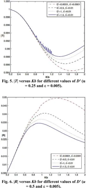
From figure 5 it is found that |T| increases as D′increases. The change in |R| and |T| for Kb > 0.7 is significant. Also, it is observed from figures 4 and 5 that |R| and |T| shows oscillatory behaviour for 0.8 < Kb < 1.2, for D′ = 1,1.5. However, for smaller values of D′ this oscillation in |R| and |T| is not significant.

Fig. 5. |T_{| versus} Kb _{for different values of} D′_(u

= 0.25 and = 0.005).

Fig. 6. |R_{| versus} Kb _{for different values of} D′₍u

= 0.5 and = 0.005).

the plate. This may be attributed to the elastic property of the ice cover. Also, this change in |R| and |T| is significant as the length of the plate diminishes.

Fig. 7. |T_{| versus} Kb _{for different values of} D′₍u

= 0.5 and = 0.005).

Fig. 8. |R_{| versus} Kb _{for small values of} u ₍D′ ₌

1.5, ′ = 0.01).

Fig. 9. |R_{| versus} Kb _{for large values of of} u ₍D′ ₌

1.5, ′ = 0.01).

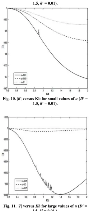
Fig. 10. |R_{| versus Kb for small values of} u ₍D′ ₌

1.5, ′ = 0.01).

Fig. 11. |T_{| versus} Kb _{for large values of} u ₍D′ ₌

1.5, ′ = 0.01.).

In figures 8-11, |R| and |T| are plotted against Kb for D′ = 1.5, = 0.005 for various lengths of the plate. It is observed from figures 8 and 9 that |R| decreases as the length of the plate decreases while figures 10 and 11 show that |T| increases with the decrease in the length of the plate for a fixed value of D′ and . Thus long plate induces more reflection of wave energy. Also for a particular length of the plate, the increase in ice cover parameter induces more transmission of wave energy.

5.

C

ONCLUSION

do not feel the presence of ice-cover as they are confined towards the bottom of the ocean. However, the short waves which are confined near the cover surface are affected by the presence of ice-cover. It is observed that long plate induces more reflection of wave energy and less transmission. Also for a particular length of the plate, the increase in ice cover parameter induces more transmission of wave energy.

A

CKNOWLEDGMENTS

SB and DM is thankful to UGC for financial support. PM is thankful to Department of Science and Technology, Government of India for their financial support of this work through the SERC Fast Track Scheme for Young Scientist (no. SR/FTP/MS-037/2011).

R

EFERENCES

Chakrabarti, A. (2000). On the solution of the prob-lem of scattering of surface water waves by the edge of an ice-cover. Proc. R. Soc. Lond. 456, 1087-1099.

Chakrabarti, A., D. S. Ahluwalia and S. R. Manam (2003). Surface water waves involving a vertical barrier in the presence of an ice-cover. Internat. J. Engng. Sci. 41, 11451162.

Chung, H. and C. Fox (2002). Calculation of wave-ice interaction using the Wiener-Hopf technique. New Zealand J. Math. 31, 1-18. Chung, H. and C. Fox (2002). Calculation of

wave-ice interaction using the Wiener-Hopf technique. New Zealand J. Math. 31, 1-18. Das, D. and B. N. Mandal (2007). Wave scattering

by a horizontal circular cylinder in a two-layer

fluid with an ice-cover. Inter. J. Eng. Sci. 45, 842-872.

Fox, C. and V. A. Squire (1994). On the oblique reflection and transmission of ocean waves at shore fast seaice. Phil. Trans. R. Soc. Lond. 347, 185-218.

Gayen, R., B. N. Mandal and A. Chakrabarti, (2005). Water wave scattering by an ice-strip. J. Eng. Math. 53, 21-37.

Kohout, A. L. and M. H. Meylan (2008). An elastic plate model for wave attenuation and ice floe breaking in the marginal ice zone. Jour. of Geophys. Res. 113.

Kundu, P. K. (1997). Diffraction of water waves by slender barriers. Journal of Engineering Mathematics 32, 87-100.

Kundu, P. K. and N. K. Saha (1998). On the scattering of water waves by a submerged sledder barrier. The Journal of Australian Mathematical Society. Series B. Applied Mathematics 40, 171-189.

Landau, L. D. and E. M. Lifshitz (1970). Theory of Elasticity. Pergamon Press 7.

Linton, C. M. and H. Chung (2003). Reflection and transmission at the ocean/sea-ice boundary. Wave Motion 38, 43-52.

Maiti, P. and B. N. Mandal (2010). Wave scattering by a thin vertical barrier submerged beneath an ice-cover in deep water. Applied Ocean Research 32, 367-373.

Maiti, P., P. Rakshit and S. Banerjea (2011). Scattering of water waves by thin vertical plate submerged below ice-cover surface. Applied Mathematics and Mechanics 32, 635-644.

Mandal, B. N. and A. Chakrabarti (1989). A note on diffraction of water waves by a nearly vertical barrier. IMA J. Appl. Math. 43, 157-165. Mandal, B. N. and P. K. Kundu (1990). Scattering of

water waves by a submerged nearly vertical plate. SIAM J. Appl. Math. 50, 1221-1231. Parsons, N. F. and P. A. Martin (1992). Scattering of

water waves by submerged plates using hypersingular integral equations. Applied Ocean Research 14, 313-321.

Shaw, D. C. (1985). Perturbational results for diffration of water waves by nearly vertical barrier. IMA J. Appl. Math. 34, 99-117. Squire, V. A. (2007). Review of ocean and sea ice

revisited. Cold Regions Science and Technology 49, 110-133.

Torri, T., H. Ohkubo, N. Hayashi, K. Matsuoka, and H. Kanai (2000). Development of a very large

floating structure. Nippon Steel Technical Report 82, 23-34.

Wadhams, P. (1978). Wave decay in the marginal ice zone measured from submarine. Deep-sea Res. 25, 23-40.

Wang, C. M., Z. Y. Tay, K. Takagi and T. Utsunomiya (2010). Review of Methods for Mitigating Hydroelastic Response of VLFS Under Wave Action. Appl. Mech. Reviews 63, 030802-18.

A

PPENDIX

A

Equation (27) involves the unknown function

0 0

( )y  ( 0, )y  ( 0, ),y

     where ₀( , )x y is the velocity potential describing the wave motion due to scattering of an incident wave by a thin vertical plate submerged in deep ocean with ice cover. This problem was studied by Maiti et al. (2011). Here we present in brief the methodology used in Maiti et al . (2011) to find ₀( , ).x y

Let us consider the function ( , )x y as

0

( , )x y



( , )x y



inc( , )x y

   A1

where ₀( , )x y satisfies BVP0 and inc( , )x y is given by (7).

2 _{0 on y 0}

    A2

4 4

{D (1 K)} y K 0 on =0y x



     

 A3

(0, ), inc

x y a y b

x 

    

 A4

1

2 _{is bounded as 0}

r  r A5 Also

( , ) as , ( , )

( 1) ( , ) as . inc

inc

R x y x

x y

T x y x

   _{  }         A6

Let G(x,y; ,η) be the source potential which de-scribes the motion in water covered with ice due to presence of a line source at ( ,η). The expression for G(x,y; ,η) is given by (32).

We now use Green’s integral theorem to the harmonic function G(x,y; ,η) and Ψ(x,y) in the region bounded by the lines y = 0, −X ≤ x ≤ X; x =±X, 0 ≤ y ≤ Y; y = Y, −X ≤ x ≤ X; x = 0±, a ≤ y ≤ b and a circle of radius ₀ with centre at ( ,η) and ultimately we make X, Y →∞ and 0 → 0 to get

2 ( ,η) b ( ) (0, ; ,η) . a

G

y y dy

x

    





A7

Noting (A1), Eq. (A7) transforms to

0

1

( ,η) ( ,η) ( ) (0, ; ,η) . 2

b inc

a

G

y y dy

x        



A8

Now using the third condition in BVP-0 in (A8) and using the relation (7), we obtain the following hypersingular integral equation after some simplifications

2 λ ( η)

2 2 4

λ ( η)

λ 4 0 2 λ 2 1

4 4 4 4 5

0

λ η

1 1 2 λ

[

( η) ( η) 5 (λ ) 1 -2K

( 1 )

2 (λ ) ( η)

] ( )

λ ( λ )

2 λ η .

K y b a k y K k x K

K i e X

y y D K K

ke

dk

k Dk K K

K K

e y x

dx y dy

K D k x Kx Kx

i Ke a b

                   _       







A9

To solve the above hypersingular integral equation we put

2 2

η .

2 2

b a b a

y t

b a b a

u      _    _   _ A10

into (A9), to obtain

1

2 1

1

( , ) ( ) ( ), 1 1 ( )

X L u t F t dt h u u

t u               



A11 Where 2 2

2 2 2 2 2

2 2 λ ( )

4 2 _λ 4 0 λ 2 2

4 4 4

( , ) ( )

4( ) 4( )( ) ( ) ( )

( ) λ

2 5 (λ ) 1

( ) 2

4 ( 1 )

( ) (λ )

2 λ ( λ

K y k K K x x L u t

b a

b a b a t u b a t u

b a K i e

D K K

b a Kk

k Dk K K

b a e

K K

K D k x Kx

                             



1 5 0 ₎



A12 ( ) 2 b a

b a t u

     A13

( ) , 1 1,

2 2

b a b a

F t  _    t_   t

  A14

( 1) 0,

F   A15 and

λ( )

2 2

( ) 2 λ ( ) 1 1.

2

b a b a

K u

b a

h u i K e u

 

 



    

A16 Following the methodology used by Parson’s and Martin (1992) we assume

2

( ) (1 ) ( )

F t  t H t A17 so that F( 1) 0.

We now approximate H(t) as

0

( ) ( ), 1 1, N

n n n

H t a U t u







   A18

where Un(t) is a Chebyshev polynomial of the second kind and aa nn( 0,1, 2,... )N are unknown constants. Using the expansion (A18) in (A17) and substituting in (A11) we obtain

0

( ) ( ), 1 1 N

n n n

a A u h u u



   



A19

Where

1

1 _{2 2}

1

( ) ( 1) ( ) (1 ) ( ) ( , ) .

n n n

A u  n U u t U t L u t dt



   

_



A 20 To find the unknown constants

( 0,1, 2,... ), n

aa n N we put

( 0,1,..., ), j

0

, 0,1, 2,..., N

n nj j n

a A h j N



 



A21

Where

( ), ( )

nj n j j j

A A u h h u A22 The collocation points u_j can be chosen suitably. Here we have chosen

( 1)

cos , 0,1, 2,..., . 2

j j

u j N

N 

 

 A23 The linear system (A22) is solved by any standard method to obtain the constants

( 0,1, 2,... ). n