ISCTE - Instituto Universitário de Lisboa BRU-IUL (Unide-IUL)
Av. Forças Armadas 1649-126 Lisbon-Portugal http://bru-unide.iscte.pt/
FCT Strategic Project UI 315 PEst-OE/EGE/UI0315
Working Paper – 12/03
An Integrated Approach for the
Measurement of Inequality, Poverty
and Richness
Nuno Crespo
Sandrina B. Moreira
1
AN INTEGRATED APPROACH FOR THE MEASUREMENT
OF INEQUALITY, POVERTY, AND RICHNESS
Nuno Crespo*, Sandrina B. Moreira† and Nádia Simões‡
*Instituto Universitário de Lisboa (ISCTE - IUL), ISCTE Business School Economics
Department, UNIDE - IUL (Business Research Unit), Lisboa, Portugal; e-mail:
†Instituto Politécnico de Setúbal (ESCE - IPS), Department of Economics and Management,
Setúbal, Portugal and UNIDE - IUL (Business Research Unit), Lisboa, Portugal; e-mail:
‡Instituto Universitário de Lisboa (ISCTE - IUL), ISCTE Business School Economics
Department, UNIDE - IUL (Business Research Unit), Lisboa, Portugal; e-mail:
nádia.simõ[email protected]
Abstract: We propose a new and integrated approach to the measurement of inequality in
income distribution, poverty, and richness. In the context of the poverty and richness
measures, we consider the three dimensions usually analysed – incidence, intensity, and
severity. The proposed broad set of indicators is easy to calculate and is based on a neutral
income inequality concept. The method also allows an objective interpretation of the values
for each measure, a decomposition according to households’ characteristics, and an immediate
comparison of the results between countries and time periods. We illustrate the application of
the measures with data from Portugal.
Key words: income inequality, poverty, richness, measurement.
2 1. Introduction
Income inequality and poverty are well established research fields in the economic literature.
Apart from a multiplicity of other empirical and theoretical contributions, several recent
books address the state of the art of the research about inequality and poverty, including
Wolff (2009), Salverda et al. (2011), and Cowell (2011). This analysis can be justified on several grounds. On the one hand is the natural wish to address an issue seen as socially
unfair. On the other hand, economic policy concerns have brought the issue of poverty and
inequality to the center of public debate, intensifying the research into their determinants. A
full knowledge of the real dimension and characterization of these phenomena is thus of
widespread interest, seeking the definition of effective socio-economic policies.
The study of top incomes has also recently emerged (Piketty, 2005; Saez and Veall, 2005;
Piketty and Saez, 2006; Roine and Waldenström, 2008; Bach et al., 2009; Atkinson and Piketty, 2010). According to Atkinson (2007) three reasons justify the analysis of the ‘rich’:
their command over resources, their command over people (income and wealth as sources of
power) and their global significance. Atkinson et al. (2011) provide a survey on this topic.
Central to all this literature has been the discussion of the procedures and indicators for
measuring income inequality, poverty, and richness. The present paper contributes to this line
of research by proposing a new methodology that allows an integrated approach for
measuring inequality, poverty, and richness.
Our approach starts from an inequality measure which is based on a concept of inequality
characterized by its neutrality, seeking to quantify the phenomenon without value judgments
on the distribution of inequality. The approach has the following characteristics: (i) simplicity
in application; (ii) an objective interpretation of the values obtained for each indicator; (iii) a
3 periods; and (iv) decomposability, i.e., the possibility of knowing the contribution of
population’s sub-groups.
The paper is structured as follows. Section 2 summarizes the main methodological issues and
indicators used in the literature. Section 3 presents the approach in which new measures of
inequality, poverty, and richness are advanced. Section 4 illustrates the application of the
proposed measures using data for Portugal. Section 5 presents some final remarks.
2. Methodological issues and indicators
For the empirical analysis of inequality, poverty, and richness, it is necessary to assume some
methodological choices as well as to select the indicator(s) that will be used. In this section,
we summarize the main options available.
2.1 Methodological issues
Measuring income inequality, poverty, and richness implies making choices concerning some
methodological issues. Four of these issues are common to the analysis of the three
phenomena while a fifth is specific to the analysis of poverty and richness. The first group
involves choices concerning: (i) the indicator of resources; (ii) the demographic unit; (iii)
equivalence scales; and (iv) the weighting of the demographic unit. In order to measure
poverty/richness, it is also necessary to define a poverty/richness line.
In relation to the indicator of resources, Cowell (2011) suggests that wealth, lifetime income,
and income are, in that order, the most adequate ones, even though none of them covers
completely the command over resources for all goods and services in society. The ease of
4 Regarding the concept of income, the most common option – given the availability of
statistical information – is the monetary disposable income. This choice is subject to criticism
because of the exclusion of non-monetary forms of income and also of the past accumulation
effect through savings and indebtedness.
The second methodological choice relates to the demographic unit, usually between the
individual and an aggregate (family or household, the latter also including individuals at the
same address who are not part of the nuclear family). The option for households is mainly
followed in the literature because of the income sharing phenomenon within the household.
Directly related to the previous option is the issue of comparing unlike units. Households with
different compositions and dimensions have distinct needs and thus require different levels of
income to achieve similar levels of well-being. The use of equivalence scales allows
calculating equivalent adults for each household. A frequently used equivalence scale is the
OECD modified scale, which gives a weight of 1 to the first adult, 0.5 to each of the
remaining adults, and 0.3 for children under 14 years of age. The income adjusted by the
composition and dimension of the household – the adult equivalent income – represents
therefore a refinement of the income per capita, not neglecting the existence of economies of scale due to the share of housing and expenses.1
Concerning the weighting of the demographic unit, the usual choice is to take the number of a
household’s individuals.
The fifth methodological issue – the poverty/richness line – is exclusive to the analysis of
poverty and richness. The main methodological question in this context is the choice between
absolute or relative lines. In the first case, the threshold is defined without reference to the
standard of living prevailing in society. In the second case, that reference is taken into
account.
1
5 2.2 Indicators
After considering the methodological questions mentioned above, one must choose the
indicators to use.
2.2.1 Inequality indicators
Four main groups of inequality indicators can be considered. The first refers to measures that
compare the income share of the top x% of the income distribution with that of the bottom
x%. Frequent values for x are 5, 10, and 20. The main advantage of this type of indicator – and the reason for its strong support (at least as a preliminary indicator) – is the ease of
calculation and interpretation. However, evaluating inequality through these measures is
limited because the income distribution inside each income group is not considered
(Haughton and Khandker, 2009).
The most widely used measure of income inequality is the well-known Gini coefficient,
which varies between 0 (total equality) and 1 (maximum inequality). However, this index is
not (easily) decomposable, which is one of its main limitations.
A third way to measure inequality is the index proposed by Atkinson (1970). Its most
important characteristic is making the value judgments involved in the measurement of
inequality explicit, by taking into account a parameter that captures the degree of inequality
aversion. That parameter can vary between 0 (inequality indifference) and +∞ (corresponding
to the Rawlsian criterion that values only the income of the poorest).
A last group of inequality indicators corresponds to the Generalized Entropy (GE) measures,
6 Similar to the Atkinson index, GE measures clearly assume the incorporated value judgments
through a parameter representing the weight attributed to income differences in different parts
of the distribution. The most common values for that parameter are 0, 1, and 2. The
inexistence of inequality implies that GE measures assume a value of 0. The increase of the
value of such indicators corresponds to an increase in inequality. GE measures are additively
decomposable, a crucial property for the evaluation of inequality determinants.
2.2.2 Poverty indicators
Several poverty measures are available in the literature, capturing the different dimensions of
this phenomenon (incidence, intensity, and severity). The headcount index (P0) captures the
first dimension, measuring the proportion of individuals classified as poor (i.e., with an
income lower than the poverty line) in the total population. The main merit of this measure is
the simplicity of calculation and interpretation. However, an important weakness of P0 is the
fact that it is only an accounting of the poor, with no sensibility regarding the magnitude of
the problem.
In its turn, the poverty gap index (P1) measures the mean deviation of income from the
poverty line, capturing the intensity of poverty. Thus P1 overcomes the main limitation of P0.
The poverty severity index (P2) is a third poverty indicator, which measures the inequality
among the poor by calculating the sum of poverty gaps weighted by the gaps themselves
(Haughton and Khandker, 2009). Thus P2 is especially affected by extreme poverty situations.
A particularly appealing way to present the three above measures of poverty is through the
7 N
Z i G
P
N
1 i
∑
⎟
⎠
⎞
⎜
⎝
⎛
=
α
α= , (1)
in which N is the total number of individuals in the population, Z the poverty line, and Gi the
poverty gap associated with individual i. Gi will be zero if the income of i ( Yi) is greater than
or equal to Z and (Z−Yi) in the opposite case (i.e., when i is poor). The parameter α (α ≥ 0)
represents the sensitivity of the index to poverty. When α is 0, 1, and 2, one obtains the
poverty measures mentioned above, that is, the headcount index, the poverty gap index, and
the poverty severity index, respectively. Decomposability is an interesting property of Pα. On the contrary, the index proposed by Sen (1976) – also attempting to capture in a single
measure the three above dimensions – does not satisfy that property. As shown by Blackwood
and Lynch (1994), the Sen index is more sensitive to a reduction in the headcount index
compared to a decrease in the poverty gap or in the inequality among the poor. Therefore, the
Sen index is somewhat biased toward policies that reduce the number of poor (Blackwood
and Lynch, 1994).
2.2.3 Richness indicators
While the methodologies used to analyse inequality and poverty are well consolidated in the
literature, this is not so for the evaluation of richness (Peichl et al., 2010). In that context, the most commonly applied measures are the income share of the top x% of the income distribution and headcount measures. As stated above, both measures have however serious
8 contribution is given by Peichl et al. (2010) who have suggested a class of richness measures analogous to the existent for the poverty measures.
3. An integrated approach for the measurement of inequality, poverty, and richness
3.1 On the concept(s) of income inequality
In the previous section we synthesized the most common methodological options for the
measurement of inequality, poverty, and richness, as well as the main indicators available,
stressing their specificities and (implicit or explicit) value judgments.
In this section we propose a new and integrated approach for measuring these phenomena.
We start by considering a new measure of income inequality. We then derive poverty and
richness measures, capturing their different dimensions (incidence, intensity, and severity).
However, ‘before trying to quantify anything one must first be clear about the concept to be
measured’ (Ravallion, 2003, p.740). We therefore start the analysis by discussing the concept
of inequality underlying the indicator that serves as our point of departure.
As argued by Bellù and Liberati (2006), ‘inequality is not a self-defining concept, as its
definition may depend on economic interpretations as well as ideological and intellectual
positions’ (Bellù and Liberati, 2006, p.2). Although an explicit discussion about the different
concepts of inequality underlying the measures available does not exist in the literature, one
can distinguish four main concepts.
A first – the simplest – associates inequality with the difference, in absolute terms, between
the current distribution and the egalitarian one (concept of inequality 1). In turn, the second and third concepts of inequality are relative measures of inequality. While the first one –
9 terms, the concept of inequality 3 also takes into account the distribution of inequality among the different receiving units. The last concept – concept of inequality 4 – explicitly incorporates welfare considerations in the measurement of inequality (e.g., Sen, 1976),
arguing that the level of income should also be considered in the assessment of this
phenomenon. A distribution B obtained from a distribution A, for example, by doubling all incomes corresponds to a better situation since it ensures a higher level of welfare.
This conceptual discussion is critical because the inequality indices used for empirical
purposes should reflect the specific concept considered. The measures that correspond to each
of the concepts presented above can be distinguished by their compliance with the principles
proposed by Fields and Fei (1978), which are usually used in the analysis of inequality
indicators, namely: (i) symmetry; (ii) population size independence; (iii) mean independence;
and (iv) Pigou-Dalton transfers principle.
The principle of symmetry requires that any measure of inequality should be invariant to
swaps of income among individuals. In turn, according to the principle of population size
independence, the inequality measure should not change in response to a replication of the
original population. The principle of mean independence requires that the index must not vary
when all the original incomes are multiplied by a constant. Finally, according to the
Pigou-Dalton transfers principle, any transfer of income from a richer to a poorer individual which
does not reverse their positions, reduces inequality.
Table 1 synthesizes the principles verified by the measures included in each of the four
concepts of inequality.
10 Given the notable differences between the various concepts of inequality it is important: (i) to
discuss which ones seem more appropriate for a proper measurement of the phenomenon; and
(ii) to justify the option assumed in the present study.
In the context of concept 1, a distribution B derived from a distribution A by multiplying all incomes by a positive constant reveals a greater degree of inequality than the original
distribution. This breach of the mean independence principle makes this concept difficult to
accept as an adequate basis for empirical measures of inequality.
According to the concept of inequality 4, the comparison of distributions A and B leads to the opposite conclusion, i.e., B is preferable because it provides a higher level of welfare. This concept is subject to criticism, however, because it captures more than what the concept of
inequality is intended to measure.
In this study we argue that the concepts of inequality 2 and 3 are the most interesting to measure inequality. It is important to note however that these concepts capture different
perspectives of the phenomenon and should not therefore be seen as alternatives but rather as
complements.
Concept 3 is the framework of the inequality measures most frequently used in the literature, such as those generally discussed in Section 1. This concept assumes the simultaneous
verification of the four principles suggested by Fields and Fei (1978). The Pigou-Dalton
principle is not, however, immune to criticism, as noted, for example, by Chateauneuf and
Moyes (2006) in a study entitled ‘measuring inequality without the Pigou-Dalton condition’.
Discussing the inclusion of this principle in most measures of inequality, the authors argue
that ‘one may however raise doubts about the ability of such a condition to capture the very
idea of inequality in general’ (Chateauneuf and Moyes, 2006, p.2).2
2
11 In this study we assume the concept of inequality 2. As a result, our inequality index does not verify the Pigou-Dalton principle. The reason for this choice stems directly from the main
distinguishing feature of this concept in comparison to concept 3 – its neutrality, i.e., the exclusion of any kind of distribution sensitivity. The measures based on this concept seek
only the quantification of the phenomenon. Following this perspective, the measure that we
suggest below aims to quantify the distance between the current distribution and the
egalitarian one, without any value judgment on the distribution of inequality. This index
measures the proportion of the total income that would be necessary to redistribute in order to
obtain equality. As suggested by Schutz (1951), ‘equality of income distribution is found
when every income-receiving unit receives its proportional share of the total income’ (Schutz,
1951, p. 107).
In addition to the neutrality that characterizes the measure of inequality and the full range of
indicators of poverty and richness derived from it, the approach developed throughout this
section has other appealing features: (i) it is an integrated perspective of inequality, poverty,
and richness; (ii) the simplicity of calculation of the suggested indicators; (iii) their
decomposability, allowing the identification of the contribution of population’s sub-groups;
and (iv) the specific economic interpretation of the values obtained, as opposed to most
available measures, whose values can only be interpreted by comparison with figures for
other countries or periods. The latter is an important feature to the extent that the several
indices provide useful information for the definition of policy interventions.
Regarding the methodological questions presented in the previous section, we assume the
most common choices concerning the second and third issues – households as recipient units
of income and an equivalence scale (namely the OECD modified scale) to account for the
12 fourth and fifth questions previously mentioned. The first option is unnecessary for the
present section. We will return to that subject in Section 3.
3.2 Income inequality
Taking into account the discussion of the previous section, our inequality index (I) is defined as:
∑
=
λ − ψ χ
= N
1 i
i i
I , (2)
in which:
∑
= =
ψ N
1 i
i i i
Y Y
(3)
and
∑
= =
λ N
1 i
i i i
D D
. (4)
N is the total number of households, Yi represents the total income of household i, and Di
expresses the number of equivalent adults in that household. Thus, ψiis the income weight of
13 in the income distribution when all households have an income share equal to their share in
terms of equivalent adults, that is, when ∀i,ψi =λi.
If we set χ = 0.5, the possible values for I are in the range [0,1[. This value for χ allows a more intuitive interpretation of the results and is thus more adequate than alternatives such as
χ = 1, according to which I would vary between 0 and 2. The open range at right is due to the
fact that the value of 1 corresponds to a situation where the full amount of income is held by
households of a zero dimension, an impossible case.
Taking into account the inequality measure, I, we can deepen the analysis, proposing poverty and richness measures. The first step is to set criteria to define if household i is poor (P), rich (R) or if it is in an intermediate situation, what we will call middle class (MC).3 These criteria
are based on the comparison between what the household has in terms of income with what it
should have, considering its dimension and composition, in order to obtain an equal
distribution of resources:
⎪ ⎪ ⎪ ⎪ ⎩ ⎪ ⎪ ⎪ ⎪ ⎨ ⎧ < ≤ ≤ > = β 1 if P υ β 1 if MC υ if R S λ ψ λ ψ λ ψ i i i i i i
i , (5)
in which
β
,υ
≥1.Once we classify each household according to its position in the income distribution, we can
obtain aggregated measures of poverty and richness.
3
14 3.3 Poverty
As seen above, a detailed analysis of poverty should take into account three dimensions:
incidence, intensity, and severity. Following the approach presented in the previous section,
we now propose poverty measures that focus on each of these dimensions. Additionally, we
discuss the case of the near poor.
We start by defining a measure of poverty incidence, POV. Defining Hi as the number of
individuals of household i, then:
∑
∑
= = =
= N
1 i
i N
) P S (
1 i
i
H H
POV i
. (6)
POV is a headcount index, indicating the percentage of individuals that belong to poor households in relation to the total number of individuals.
Following, we define an index of poverty intensity (POV’). Let us start by calculating θi,
which expresses the percentage of the total income in the economy that household i would have to receive to become non-poor:
i i i β −ψ
λ =
θ . (7)
15
∑
= = θ = N ) P S ( 1 i i i 'POV . (8)
If we divide POV’ by the number of poor households, we obtain an indicator of the average intensity of poverty.
The third dimension of poverty that needs to be taken into account is its severity. To capture
this dimension, we consider a set of indicators that aim to reflect different aspects of the
phenomenon. In this context, the first step of our analysis is the definition of a new poverty
threshold reflecting a higher degree of resource privation. Therefore, a situation of extreme
poverty is defined as:
ζβ < λ ψ
=SP if 1
S
i i
i , (9)
in which
ζ
>1.With reference to this line of extreme poverty, we can quantify the incidence and intensity of
severe poverty. The incidence of severe poverty can be defined in relation to either the total
population or the poor population, being expressed, respectively, as follows:
16
∑
∑
= = == = − N ) P S ( 1 i i N ) SP S ( 1 i i i i H H ) 2 ( POVS . (11)
In a similar vein, the intensity of severe poverty can be calculated by reference to either the
poverty line or the severe poverty line, being measured, respectively, as:
∑
== θ = − N ) SP S ( 1 i i i ) 1 ( ' POVS (12)
and
∑
= = ω = − N ) SP S ( 1 i i i ) 2 ( ' POVS , (13)
in which θi corresponds to its expression in (7) and:
i i i ζβ−ψ
λ =
ω . (14)
The measures of severe poverty intensity express the percentage of the total income in the
economy that would be necessary to transfer to the extreme poor in order to take them out of
poverty (in the case of S-POV’(1)) or severe poverty (in the case of S-POV’(2)).
To complement the analysis of the severity of poverty, we can calculate an inequality index
17
∑
= = ρ − η = N ) P S ( 1 i i i P i kI , (15)
in which:
∑
== = η N ) P S ( 1 i i i i i Y Y, (16)
and
∑
== = ρ N ) P S ( 1 i i i i i D D. (17)
This indicator quantifies the percentage of the total income of poor households that has to be
re-affected among them in order to obtain an equal intensity of poverty. An increase in IP
reflects higher levels of poverty severity.
Finally, let us consider the case of the near poor. An effective poverty policy cannot focus
only on the poor, but should, in line with the analysis of poverty vulnerability (Pritchett et al., 2000; Guimarães, 2007; Zhang and Wan, 2009; Dutta et al., 2011), also give special attention to those who are very near of being poor in order to avoid new poverty cases. Accordingly,
we propose measures to capture the importance of this phenomenon. We define:
ε < λ ψ ≤ β = + i i i 1 if P
18 in which
1
≤
ε
<
1
β
.Near-poverty incidence, representing the percentage of total individuals that belong to
near-poor households, is given by:
∑
∑
= = = += + N 1 i i N ) P (S 1 i i H H POV i. (19)
In this context, it is also interesting to know the safety net of the near-poor population. For
household i, that safety margin is given by the symmetric of θi. In overall terms, we quantify
this as:
∑
∑
+ + == = = + θ − = ⎟ ⎠ ⎞ ⎜ ⎝ ⎛ β λ − ψ = N ) P S ( 1 i i N ) P S ( 1 i i i i i ) (POV
'
, (20)expressing the percentage of the total income in the economy by which the near-poor are
above the poverty line. The average safety margin of near-poor can be obtained dividing
POV’+ by the number of near-poor households.
3.4 Richness
The indicators used in the analysis of poverty can be adapted for the measurement of the
19 measures of richness.4 For terminological reasons, we opt to designate the last case as
‘richness depth’.
We define RICH as the ratio between the number of individuals in rich households and the total number of individuals:
∑
∑
= = =
= N
1 i
i N
) R S (
1 i
i
H H
RICH i
. (21)
To obtain a measure of richness intensity, we define:
i i i =ψ υλ
δ − . (22)
Then, richness intensity is given by:
∑
= =δ
= N
) R S (
1 i
i
i
'
RICH , (23)
representing the percentage of the total income in the economy according to which the rich
are above the richness line. Dividing RICH’ by the number of rich households we can obtain the average intensity of richness.
Finally, we attend to richness depth. We do so using the same approach we have applied in
the poverty case. As a first step, we define an extreme richness line, above which households
are classified as extremely rich:
4
20 συ > λ ψ = i i i ER if
S , (24)
in which σ>1.
The incidence of extreme richness can be expressed in relation to either the total population or
the rich population. In each case we have, respectively:
∑
∑
= == = − N 1 i i N ) ER S ( 1 i i H H ) 1 ( RICH E i (25) and∑
∑
== == = − N ) R S ( 1 i i N ) ER S ( 1 i i i i H H ) 2 ( RICHE . (26)
In turn, taking as reference either the richness line or the extreme richness line, the intensity
of extreme richness can be defined respectively as:
∑
== δ = − N ) ER S ( 1 i i i ) 1 ( ' RICHE (27)
and
∑
== ϕ = − N ) ER S ( 1 i i i ) 2 ( ' RICH21 where δiis expressed in (22) and:
i i
i =ψ συλ
ϕ − . (29)
As in the case of the severity of poverty, we can also calculate an inequality measure applied
exclusively to the rich population, aiming to determine the amount of income that it is
necessary to redistribute among the rich in order to equalize the distance of each rich
individual to the richness line:
∑
= = μ − ϖ φ = N ) R S ( 1 i i i R iI , (30)
in which:
∑
== = ϖ N ) R S ( 1 i i i i i Y Y, (31)
and
∑
= = = μ N ) R S ( i 1i i i i D D
22 3.5 Middle class inequality
As mentioned above, the evaluation of richness has recently joined the well-established
analyses of inequality and poverty. Least explored has been the study of income distribution
in the middle class. However, this is also a relevant issue since the degree of inequality in this
income group is an important indicator of countries’ economic and social cohesion.5
To conceive such an indicator, we start by focusing on households in which Si= MC,
calculating:
∑
== ο − ϑ τ = N ) MC S ( 1 i i i MC iI , (33)
in which:
∑
= = = ϑ N ) MC S ( 1 i i i i i Y Y, (34)
and
∑
== = ο N ) MC S ( 1 i i i i i D D. (35)
5
23
MC
I is an income inequality measure for the middle class, indicating the percentage of the
total income of the middle class that, if adequately redistributed among middle class
households, would eliminate the inequality in this income group.
4. Inequality, poverty, and richness – an application with evidence from Portugal
4.1 Data and empirical evidence
In order to illustrate the application of the set of measures presented in the previous section,
we consider data from Portugal, since it is among the European countries with the highest
levels of inequality and poverty. According to the European Union Statistics on Income and
Living Conditions (EU-SILC), in 2008, Portugal was the fourth country in the EU-27 with the
highest level of inequality and the fifth country in the EU-15 with the highest level of poverty
(10th position considering the EU-27).
We use micro-data on the income and structure of households living in Portugal from the
Office of National Statistics (INE)’s Household Budget Survey (IDEF).6 We use the last
available wave of that survey, of 2005/2006.7 The results are based on a representative sample
of the Portuguese economy with 10,403 households and a total of 28,359 individuals. The
IDEF is a large-dimension survey associated with a questionnaire filled in by households with
detailed information on the whole set of collective and individual expenditures. It also
includes demographic data, income data, and data on non-frequently consumed goods and
services.
6
Statistics on household budgets is information followed at an European level – Household Budget Survey.
7
24 The subsequent analysis takes into account not only monetary income but also total income.
The comparison of the results is particularly important for two reasons: (i) the relative weight
of non-monetary income (approximately 19% of total income); and (ii) the asymmetry in the
non-monetary income distribution.
Table 2 presents the results of the application of the proposed indicators taking as a reference
the following values for the parameters: χ=0.5, β=2, υ=2, ζ=2, κ=0.5, ε=0.6, σ=2, φ=0.5, and
τ=0.5.
[Table 2]
Focusing on the results based on total income, we find the need to redistribute 23.78% of the
total income in the economy to reach a situation of equality in income distribution. It is
important to note, however, that such an overall value presupposes an adequate redistribution
of income, that is, one that does not waste resources.
Regarding the distribution of individuals by income groups, we conclude that 17.78% are
poor, 7.03% are rich, and the remaining 75.19% are from the middle class. Concentrating on
the bottom of the income distribution, we see that 10.41% of the poor (corresponding to
1.85% of the total population) face a situation of severe poverty. Additionally, individuals that
can be classified as near-poor comprise 10.52% of the total population. Finally, when
focusing on the top of the income distribution, we identify 10.98% of the rich (0.77% of the
total population) exhibiting an extreme richness situation.
The analysis of poverty intensity allows us to conclude that a value equivalent to 2.09% of the
total income in the economy is necessary to eliminate it. That amount includes a fraction of
0.54% of the total income in the economy corresponding to what is necessary in order to
25 Only 0.09% of the total income in the economy would be needed to improve the situation of
these households to the level of the severe poverty line. A complementary way of analyzing
the level of inequality among the poor population is to apply an inequality measure
exclusively to the poor. In that case, we observe a need to re-affect (at least) 9.58% of the
poor income to remove that inequality and thus have the different poor households at the
same distance from the poverty line. In addition, the near-poor possess, as a whole, a safety
net equivalent to 0.54% of the total income.
Concerning the evaluation of richness, the income surplus from the richness line equals
7.18% of the total income. A value equivalent to 3.17% of that total income is the amount
needed to reduce the income of the extremely rich to the richness line level. That income
reduction to the level of the extreme richness line implies the movement of 1.59% of the total
income in the economy. The measurement of richness inequality indicates the need to
re-affect 13.88% of the total income of the rich population in order to eliminate that inequality.
Finally, looking at the middle class, we find that 14.97% of the income in middle-class
households would have to be redistributed among them to ensure total income equality for the
middle-class.
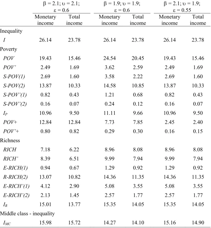
The concrete results obtained naturally depend on the values assumed for the different
parameters. However, there are no valid reasons to unequivocally support certain values for
those parameters, namely the ones that are a reference for the definition of the income groups.
They are explicitly and subjectively defined by the researcher and thus sensitivity analyses
based on alternative values are welcomed. A preliminary analysis of the kind is presented in
annex Table A.1 considering other values for β, υ, and ε.8
8
26 4.2 Decomposition by households’ characteristics – an example
As stressed above, the measures proposed in Section 2 allow their decomposition by any
household’s characteristic, such as type of household (dimension and composition), region of
residence, or variables associated with the individual of reference of that household (i.e., the
individual with the largest proportion of the annual net total income of the household), such as
age, gender, educational level, labour market state, amongst others. We have conducted a
decomposition by region of residence to illustrate that possibility. This exercise allows
focusing on the existence of regional inequalities in Portugal for the dimensions analysed in
this paper.
[Table 3]
Table 3 illustrates the decomposition by region of all the measures calculated in Table 2.
Additionally, the last row presents evidence in relation to
∑
= ψ −λ
N
1 i
i
i )
( , allowing us to
emphasize the regions where households’ weight in terms of income exceeds their respective
weight in terms of dimension.
The reading of both incidence and intensity indicators is immediate. The value corresponding
to each region should be interpreted in the same way as the overall indicator, though applied
exclusively to the given region. Let us consider the poverty indicators as examples. Regarding
POV, we found a poverty incidence at the national level of 17.78%. A disaggregation by regions reveals that 3.99% of the individuals from the sample are poor living in the Norte
27 however that this concept is different from the measurement of poverty incidence within the
context of each given region.
In the same vein, regarding POV’, we can say, for instance, that the amount necessary to eradicate poverty in the Algarve corresponds to (at least) 0.25% of the total income in the economy, while for Madeira that value is equivalent to 0.40% of the total income in the economy. In the national total, as has been seen, a mobilization of 2.09% of the total income
in the economy is needed to overcome poverty. The interpretation made for the values of POV
and POV’ is also valid for the other incidence or intensity indicators – S-POV(1), S-POV(2),
S-POV’(1), S-POV’(2), POV+, POV’+, RICH, RICH’, E-RICH(1), E-RICH(2), E-RICH’(1), and E-RICH’(2).
Concerning the inequality indicators (I, IP, IR, and IMC), the value for each region expresses
half of the deviation assigned to households of that region in relation to an egalitarian
situation (having the same weight in terms of income and equivalent adults). So, for instance,
taking into account the overall indicator of inequality (I), the deviation from the egalitarian situation of households living in the Norte region equals 8.82% of the total income in the economy.
The percentage of the total income in the economy needed to eradicate inequality within each
region cannot, in this case, be identified, because there are inter-regional transfers of income
apart from intra-regional transfers. The transfers between regions are net positive amounts
transferred to other regions when
∑
= ψ −λ
N
1 i
i
i )
( > 0 and net positive amounts received from
other regions in the opposite case.
28 5. Final remarks
The main contribution of this paper is the proposal of an integrated approach for the
measurement of inequality, poverty, and richness. We have proposed a set of indicators
characterized by their simplicity in application, neutrality, and decomposability. Another
important characteristic of the measures proposed in this study is the fact that they allow a
concrete economic interpretation of the results, thereby contributing to a more adequate
definition of social policies.
The proposed measures were applied, for illustrative purposes, to the Portuguese economy.
Taking total income as a reference, that application has identified 17.78% of individuals in
poor households, 7.03% in rich households, and the remaining 75.19% in the middle class. A
severe poverty situation was found in 1.85% of the individuals analysed (10.41% of the poor).
Particularly important in quantitative terms is the near-poverty phenomenon, accounting for
10.52% of the population. Concerning inequality, we have calculated the need to re-affect (at
least) 23.78% of the total income in the economy to reach a full equality situation. With a
focus on poverty intensity, we conclude that 2.09% of the total income in the economy is the
amount needed to be transferred from the non-poor to the poor in order to eradicate poverty.
Additionally, the comparison between the results obtained with monetary income and total
income stresses significant differences, highlighting the importance of taking into account this
last concept of income.
The proposed measures can be decomposed with reference to a given characteristic of the
household. We have illustrated that property by considering a regional decomposition that
29
Lisboa (the most developed region in the country) to be the most favourable in terms of poverty and richness.
Regarding the topics developed in this paper, important research avenues remain. In
methodological terms, the main challenge resides in testing the robustness of the results based
on alternative values for the parameters in order to check the sensitivity of these results. This
is especially important for the parameters that distinguish the main income categories (β, υ, ζ,
σ, and ε), that is, poor, rich, middle class, severe poor, extremely rich, and near-poor.
In applied terms, cross-country comparative studies also enable raising the knowledge on the
phenomena under examination for a wide range of countries with distinct characteristics. The
same comparative analysis could be conducted at the regional level, emphasizing the regional
inequalities prevailing within a given country
Acknowledgements
We thank the Office of National Statistics (INE) for kindly providing us with the survey data.
The usual disclaimer applies.
Funding
Fundação para a Ciência e a Tecnologia (FCT PEst-OE/EGE/UI0315/2011).
References
Amiel, Y. and Cowell, F. (1992) Measurement of income inequality: experimental test by
questionnaire, Journal of Public Economics, 47, 3-26.
Atkinson, A. (1970) On the measurement of income inequality, Journal of Economic Theory, 2, 244-63.
Atkinson, A. (2007) Measuring top incomes: methodological issues, in A. Atkinson and T.
30 Atkinson, A. and Brandolini, A. (2011) On the identification of the ‘middle class’, Working
Paper No. 2011-217, The Society for the Study of Economic Inequality.
Atkinson, A. and Piketty, T. (2010) Top Incomes: A Global Perspective, Oxford University Press, Oxford.
Atkinson, A., Piketty, T. and Saez, E. (2011) Top incomes in the long run of history,
Journal of Economic Literature, 49, 3-71.
Bach, S., Corneo, G. and Steiner, V. (2009) From bottom to top: the entire income
distribution in Germany, 1992-2003, Review of Income and Wealth, 55, 303-30.
Bellù, L. and Liberati, P. (2006) Inequality and axioms for its measurement, EasyPol
module No. 054, Food and Agriculture Organization of the United Nations.
Blackwood, D. and Lynch, R. (1994) The measurement of inequality and poverty: a policy
maker’s guide to the literature, World Development, 22, 567-78.
Chateauneuf, A. and P. Moyes (2006) Measuring inequality without the Pigou-Dalton
condition, in M. McGillivray (ed.) Inequality, poverty and well-being, Palgrave MacMillan, New York.
Cowell, F. (2011) Measuring Inequality, 3rd edn, Oxford University Press, Oxford.
Cowell, F. and Kuga, K. (1981a) Additivity and the entropy concept: an axiomatic approach
to inequality measurement, Journal of Economic Theory, 25, 131-43.
Cowell, F. and Kuga, K. (1981b) Inequality measurement: an axiomatic approach, European Economic Review, 15, 287-305.
Dutta, I., Foster, J. and Mishra, A. (2011) On measuring vulnerability to poverty, Social Choice and Welfare, 37, 743-61.
Eisenhauer, J. (2011) The rich, the poor, and the middle class: thresholds and intensity
indices, Research in Economics, 65, 294-304.
Fields, G. and Fei, J. (1978) On inequality comparisons, Econometrica, 46, 305-16.
Foster, J., Greer, J. and Thorbecke, E. (1984) A class of decomposable poverty measures,
Econometrica, 52, 761-76.
Gaertner, W. and C. Namezie (2003) Income inequality, risk, and the transfer principle: a
31 Gigliarano, C. and Mosler, K. (2009) Measuring middle-class decline in one and many
attributes, Working Paper No. 333, Università Politecnica delle Marche.
Guimarães, R. (2007) Searching for the vulnerable: a review of the concepts and assessments
of vulnerability related to poverty, European Journal of Development Research, 19, 234-50. Haddad, L. and Kanbur, R. (1990) How serious is the neglect of intra-household
inequality?, Economic Journal, 100, 866-81.
Harrison, E. and Seidl, C. (1994) Perceptional inequality and preference judgments: an
empirical examination of distributional axioms, Public Choice, 79, 61-81.
Haughton, J. and Khandker, S. (2009) Handbook on Poverty and Inequality, World Bank Publications, Washington.
Magdalou, B. and Moyes, P. (2009) Deprivation, welfare and inequality, Social Choice and Welfare, 32, 253-73.
Magdalou, B. and Nock, R. (2011) Income distributions and decomposable divergence
measures, Journal of Economic Theory, 146, 2440-54.
Medeiros, M. (2006) The rich and the poor: the construction of an affluence line from the
poverty line, Social Indicators Research, 78, 1-18.
Peichl, A., Schaefer, T. and Scheicher, C. (2010) Measuring richness and poverty: a micro
data application to Europe and Germany, Review of Income and Wealth, 56, 597-619.
Piketty, T. (2005) Top income shares in the long run: an overview, Journal European Economic Association, 3, 382-92.
Piketty, T. and Saez, E. (2006) The evolution of top incomes: a historical and international
perspective, American Economic Review, 96, 200-5.
Pritchett, L., Suryahadi, A. and Sumarto, S. (2000) Quantifying vulnerability to poverty - a
proposed measure, applied to Indonesia, Policy Research Working Paper Series No. 2437,
The World Bank.
Ravallion, M. (2003) The debate on globalization, poverty and inequality: why measurement
matters, International Affairs, 79, 739-53.
Roine, J. and Waldenström, D. (2008) The evolution of top incomes in an egalitarian
32 Saez, E. and Veall, M. (2005) The evolution of high incomes in Northern America: lessons
from Canadian evidence, American Economic Review, 95, 831-49.
Salverda, W., Nolan, B. and Smeeding, T. (2011) The Oxford Handbook of Economic Inequality, Oxford University Press, Oxford.
Schutz, R. (1951) On the measurement of income inequality, American Economic Review, 41, 107-22.
Sen, A. (1976) Poverty: an ordinal approach to measurement, Econometrica, 44, 219-31. Winkelmann, L. and Winkelmann, R. (2010) Does inequality harm the middle class?,
Kyklos, 63, 301–16.
Wolff, E. (2009) Poverty and Income Distribution, 2nd edn, Wiley-Blackwell, Oxford.
Zhang, Y. and Wan, G. (2009) How precisely can we estimate vulnerability to poverty?,
33 Table 1: Inequality concepts and the principles proposed by Fields and Fei (1978)
Principles
Inequality concept
Symmetry Population size
independence
Mean
independence
Pigou-Dalton
transfers principle
Concept 1 Yes Yes No No
Concept 2 Yes Yes Yes No
Concept 3 Yes Yes Yes Yes
34 Table 2: Inequality, poverty, and richness indicators for Portugal (%)
Monetary income Total income
Inequality
I 26.14 23.78
Poverty
POV 21.85 17.78
POV’ 2.99 2.09
S-POV(1) 3.13 1.85
S-POV(2) 14.31 10.41
S-POV’(1) 1.00 0.54
S-POV’(2) 0.20 0.09
IP 11.04 9.58
POV+ 10.42 10.52
POV’+ 0.52 0.54
Richness
RICH 7.94 7.03
RICH’ 9.15 7.18
E-RICH(1) 1.09 0.77
E-RICH(2) 13.77 10.98
E-RICH’(1) 4.56 3.17
E-RICH’(2) 2.33 1.59
IR 15.14 13.88
Middle class - inequality
IMC 15.19 14.97
35 Table 3: Regional decomposition of inequality, poverty, and richness indicators
Region
Index
Norte Centro Lisboa Alentejo Algarve Açores Madeira ∑
Inequality
I 4.41 3.45 4.09 3.04 3.40 2.44 2.97 23.78
Poverty
POV 3.99 2.60 1.47 2.44 2.02 2.02 3.23 17.78
POV’ 0.42 0.33 0.19 0.30 0.25 0.20 0.40 2.09
S-POV(1) 0.45 0.21 0.16 0.20 0.21 0.14 0.48 1.85
S-POV(2) 2.54 1.19 0.87 1.13 1.17 0.79 2.72 10.41
S-POV’(1) 0.13 0.07 0.05 0.07 0.06 0.04 0.13 0.54
S-POV’(2) 0.021 0.011 0.011 0.013 0.010 0.005 0.021 0.09
IP 2.13 1.44 0.78 1.44 1.08 0.91 1.80 9.58
POV+ 2.44 1.76 0.56 1.79 1.21 1.04 1.71 10.52
POV’+ 0.13 0.09 0.03 0.10 0.06 0.05 0.08 0.54
Richness
RICH 1.13 0.84 1.87 0.69 1.16 0.81 0.52 7.03
RICH’ 0.97 1.00 2.54 0.47 0.99 0.85 0.38 7.18
E-RICH(1) 0.13 0.09 0.31 0.04 0.09 0.09 0.03 0.77
E-RICH(2) 1.81 1.30 4.36 0.50 1.30 1.30 0.40 10.98
E-RICH’(1) 0.41 0.48 1.32 0.11 0.30 0.46 0.08 3.17
E-RICH’(2) 0.16 0.27 0.69 0.04 0.11 0.28 0.03 1.59
IR 2.10 1.81 4.33 1.05 1.96 1.90 0.73 13.88
Middle class - inequality
IMC 2.85 2.21 1.96 2.21 2.29 1.40 2.05 14.97
∑( - )
N
1 i
i i
=
λ
ψ -1.74 -0.72 4.37 -1.22 0.96 0.34 -1.99 0
36 Annex
Table A.1: Inequality, poverty, and richness indicators for Portugal using both
monetary and total income – sensitivity tests
β = 2.1; υ = 2.1;
ε = 0.6
β = 1.9; υ = 1.9;
ε = 0.6
β = 2.1; υ = 1.9;
ε = 0.55 Monetary
income
Total income
Monetary income
Total income
Monetary income
Total income Inequality
I 26.14 23.78 26.14 23.78 26.14 23.78
Poverty
POV 19.43 15.46 24.54 20.45 19.43 15.46
POV’ 2.49 1.69 3.62 2.59 2.49 1.69
S-POV(1) 2.69 1.60 3.58 2.22 2.69 1.60
S-POV(2) 13.87 10.33 14.58 10.85 13.87 10.33
S-POV’(1) 0.82 0.43 1.21 0.68 0.82 0.43
S-POV’(2) 0.16 0.07 0.24 0.12 0.16 0.07
IP 10.96 9.50 11.11 9.66 10.96 9.50
POV+ 12.84 12.84 7.73 7.85 2.45 2.40
POV’+ 0.80 0.82 0.29 0.30 0.16 0.15
Richness
RICH 7.18 6.22 8.96 8.08 8.96 8.08
RICH’ 8.39 6.51 9.99 7.94 9.99 7.94
E-RICH(1) 0.94 0.67 1.29 0.92 1.29 0.92
R-RICH(2) 13.07 10.82 14.36 11.35 14.36 11.35
E-RICH’(1) 4.12 2.90 5.08 3.55 5.08 3.55
E-RICH’(2) 2.13 1.45 2.57 1.77 2.57 1.77
IR 15.01 13.77 15.35 14.05 15.35 14.05
Middle class - inequality