DEPARTAMENTO DE TELEINFORMÁTICA
PROGRAMA DE PÓS GRADUAÇÃO EM ENGENHARIA DE TELEINFORMÁTICA
DANIEL COSTA ARAÚJO
CHANNEL ESTIMATION TECHNIQUES APPLIED TO MASSIVE MIMO SYSTEMS USING SPARSITY AND STATISTICAL APPROACHES
CHANNEL ESTIMATION TECHNIQUES APPLIED TO MASSIVE MIMO SYSTEMS USING SPARSITY AND STATISTICAL APPROACHES
Tese de doutorado apresentada ao Curso de En-genharia de Teleinformática da Universidade Fe-deral do Ceará, como requisito parcial para ob-tenção do Título de Doutor em Engenharia de Teleinformática.
Orientador: Prof. Dr.João César Moura Mota
Co-Orientador: Prof. Dr. André Lima Férrer de Almeida
Gerada automaticamente pelo módulo Catalog, mediante os dados fornecidos pelo(a) autor(a)
A688c Araújo, Daniel Costa.
Channel Estimation Techniques Applied to Massive MIMO Systems Using Sparsity and Stastistical Approaches / Daniel Costa Araújo. – 2016.
124 f. : il. color.
Tese (doutorado) – Universidade Federal do Ceará, Centro de Tecnologia, Programa de Pós-Graduação em Engenharia de Teleinformática, Fortaleza, 2016.
Orientação: Prof. Dr. João César Moura Mota.
Coorientação: Prof. Dr. André Lima Férrer de Almeida.
1. Massive MIMO. 2. Channel estimation. 3. Compressive Sensing. 4. Hybrid Beamforming. 5. Sparsity. I. Título.
CHANNEL ESTIMATION TECHNIQUES APPLIED TO MASSIVE MIMO SYSTEMS USING SPARSITY AND STATISTICAL APPROACHES
Tese de doutorado apresentada ao Curso de Engenharia de Teleinformática da Univer-sidade Federal do Ceará, como requisito parcial para obtenção do Título de Doutor em Engenharia de Teleinformática.
Aprovada em 29/10/2016
BANCA EXAMINADORA
Prof. Dr.João César Moura Mota (Orientador) Universidade Federal do Ceará (UFC)
Prof. Dr. André Lima Férrer de Almeida (Co-Orientador)
Universidade Federal do Ceará (UFC)
Prof. Dr.Charles Casemiro Cavalcante Universidade Federal do Ceará (UFC)
Prof. Dr. Sérgio Lima Neto Universidade Federal do Rio de Janeiro
I am very thankful to everyone that has supported me in my Doctor of Philosophy (PhD) period. I could not have done this thesis alone.
First of all, my thanks are to my advisor and co-advisor Dr. João César Moura Mota and Dr. André Lima F. de Almeida, respectively. Prof. Dr. João César has a history in my academic career. He accepted me as his Master student in 2010, and since ever he has helped by providing guidance, trust and advises in my academic career. I am also grateful to my co-advisor Prof. Dr. André Lima for his knowledge, teachings, technical discussion and incentive in producing papers and participating in research projects. Both Prof. Dr. João César and Prof. Dr. André Lima have a large contribution to my academic career.
My gratitude is also extended to my colleagues in the Wireless Telecommunication Research Group (GTEL). The group gave me the opportunity of working in two Ericsson’s projects. In such projects, the team has given me a lot of inputs in technical discussions and has also contributed a lot to build my understanding on telecommunication systems. The outcomes from those fruitful discussions are part of this thesis today and, for the people that I have had the pleasure of working with, I must say thank you for your contributions on this thesis. Besides this, I must also express my thanks to Prof. Dr. Francisco Rodrigo Porto Cavalcanti who has accepted me in the projects and gave me his trust by offering me the chance to be an intern at Ericsson. The internship was indeed a very important part of the process to achieve the PhD degree.
Ericsson and CAPES have provided all the conditions to financially supporting my internships at Ercisson Research in Sweden. As an intern, I had the opportunity of working with remarkable researchers in the Department of Radio Access Technology (RAT). The people in RAT contributed a lot with their knowledge, technical discussions and their simulators which helped me to generate many of the results in this thesis.
To the last, but not least, I have special thanks to my family, especially to my parents Moisés David Façanha Araújo and Nágila Costa Araújo. They gave me incentive since ever by supporting me whenever I needed. This thesis would not be possible without them. I am also thankful to my beloved fiancé and future wife, Nicole Marques Sousa, who has been with me during this period and has been a source of inspiration to me.
Massive MIMO has the potential of greatly increasing the system spectral efficiency by employ-ing many individually steerable antenna elements at the base station (BS). This potential can only be achieved if the BS has sufficient channel state information (CSI) knowledge. The way of acquiring it depends on the duplexing mode employed by the communication system. Currently, frequency division duplexing (FDD) is the most used in the wireless communication system. However, the amount of overhead necessary to estimate the channel scales with the number of antennas which poses a big challenge in implementing massive MIMO systems with FDD protocol. To enable both operating together, this thesis tackles the channel estimation problem by proposing methods that exploit a compressed version of the massive MIMO channel. There are mainly two approaches used to achieve such a compression: sparsity and second order statistics. To derive sparsity-based techniques, this thesis uses a compressive sensing (CS) framework to extract a sparse-representation of the channel. This is investigated initially in a flat channel and afterwards in a frequency-selective one. In the former, we show that the Cramer-Rao lower bound (CRLB) for the problem is a function of pilot sequences that lead to a Grassmannian matrix. In the frequency-selective case, a novel estimator which combines CS and tensor analysis is derived. This new method uses the measurements obtained of the pilot subcarriers to esti-mate a sparse tensor channel representation. Assuming a Tucker3 model, the proposed solution maps the estimated sparse tensor to a full one which describes the spatial-frequency channel response. Furthermore, this thesis investigates the problem of updating the sparse basis that arises when the user is moving. In this study, an algorithm is proposed to track the arrival and departure directions using very few pilots. Besides the sparsity-based techniques, this thesis investigates the channel estimation performance using a statistical approach. In such a case, a new hybrid beamforming (HB) architecture is proposed to spatially multiplex the pilot sequences and to reduce the overhead. More specifically, the new solution creates a set of beams that is jointly calculated with the channel estimator and the pilot power allocation using the minimum mean square error (MMSE) criterion. We show that this provides enhanced performance for the estimation process in low signal-noise ratio (SNR) scenarios.
Pesquisas em sistemas MIMO massivo (do inglês multiple-input multiple-output) ganharam muita atenção da comunidade científica devido ao seu potencial em aumentar a eficiência espec-tral do sistema comunicações sem-fio utilizando centenas de elementos de antenas na estação de base (EB). Porém, tal potencial só poderá é obtido se a EB possuir suficiente informação do estado de canal. A maneira de adquiri-lo depende de como os recursos de comunicação tempo-frequência são empregados. Atualmente, a solução mais utilizada em sistemas de comunicação sem fio é a multiplexação por divisão na frequência (FDD) dos pilotos. Porém, o grande desafio em implementar esse tipo solução é porque a quantidade de tons pilotos exigidos para estimar o canal aumenta com o número de antenas. Isso resulta na perda do eficiência espectral prometido pelo sistema massivo. Esta tese apresenta métodos de estimação de canal que demandam uma quantidade de tons pilotos reduzida, mas mantendo alta precisão na estimação do canal. Esta redução de tons pilotos é obtida porque os estimadores propostos exploram a estrutura do canal para obter uma redução das dimensões do canal. Nesta tese, existem essencialmente duas abor-dagens utilizadas para alcançar tal redução de dimensionalidade: uma é através da esparsidade e a outra através das estatísticas de segunda ordem. Para derivar as soluções que exploram a esparsidade do canal, o estimador de canal é obtido usando a teoria de “compressive sensing” (CS) para extrair a representação esparsa do canal. A teoria é aplicada inicialmente ao problem de estimação de canais seletivos e não-seletivos em frequência. No primeiro caso, é mostrado que limitante de Cramer-Rao (CRLB) é definido como uma função das sequências pilotos que geram uma matriz Grassmaniana. No segundo caso, CS e a análise tensorial são combinado para derivar um novo algoritmo de estimatição baseado em decomposição tensorial esparsa para canais com seletividade em frequência. Usando o modelo Tucker3, a solução proposta mapeia o tensor esparso para um tensor cheio o qual descreve a resposta do canal no espaço e na frequência. Além disso, a tese investiga a otimização da base de representação esparsa propondo um método para estimar e corrigir as variações dos ângulos de chegada e de partida, causados pela mobilidade do usuário. Além das técnicas baseadas em esparsidade, esta tese investida aquelas que usam o conhecimento estatístico do canal. Neste caso, uma nova arquitetura debeamforminghíbrido é proposta para realizar multiplexação das sequências pilotos. A nova solução consite em criar um conjunto de feixes, que são calculados conjuntamente com o estimator de canal e alocação de potência para os pilotos, usand o critério de minimização erro quadrático médio. É mostrado que esta solução reduz a sequencia pilot e mostra bom desempenho e cenários de baixa relação sinal ruído (SNR).
Figure 1.1 – The architecture of a heterogeneous network. . . 17
Figure 1.2 – The FDD system is composed of two channels: uplink and downlink. The user equipment (UE) estimates the channel by using the pilot sequence sent in the downlink channel, then reports channel estimation in the feedback channel (uplink channel). . . 18
Figure 1.3 – Diagram of the thesis organization. . . 21
Figure 2.1 – Plot of a functionkθkp∀p∈[0,1], whereθ∈R. . . 28
Figure 2.2 – Centralized channel estimation solution using greedy algorithm. . . 36
Figure 2.3 – Alternated channel estimation using alternate direction method of multipliers (ADMM) solution. . . 38
Figure 2.4 – Distributed channel estimation solution using ADMM in each module. . . . 40
Figure 2.5 – Channel estimation performance of distributed ADMM, centralized ADMM and OMP for a128×2multiple-input multiple-output (MIMO) using system T = 40. . . 41
Figure 2.6 – Channel estimation performance for a128×2MIMO system considering signal-noise ratio (SNR) =35dB. . . 42
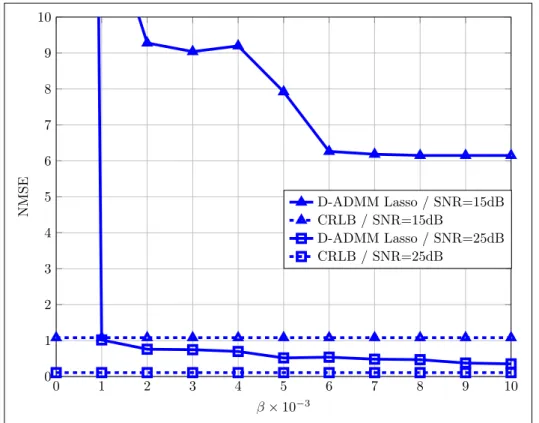
Figure 2.7 – Channel estimation performance of D-ADMM in a128×2MIMO system. In this plot, we vary the parameterβ. . . . 43
Figure 3.1 –n-Mode product representation for a third order tensor model. . . . 48
Figure 3.2 – Third-order tucker decomposition of a sparse tensor. . . 49
Figure 3.3 – Power delay profile considered to create a wideband channel. . . 59
Figure 3.4 – Channel estimation result with a pilot placement configuration that uses 34 regularly spaced pilot subcarriers which carry sequences withN = 40. . . . 60
Figure 3.5 – Channel estimation result with a pilot placement configuration that uses 10 regularly spaced pilot subcarriers which carry sequences withN = 40. . . . 60
Figure 3.6 – Channel estimator performance varying the number of subcarriers. . . 61
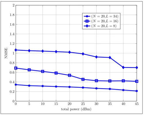
Figure 3.7 – Channel estimator performance by varying the transmit power for some pilot placement configurations. . . 61
Figure 4.1 – Proposed channel estimation to identify strongest multipaths using multiple subcarriers. . . 69
Figure 4.2 – Pilot distribution on the time-frequency grid. . . 75
Figure 4.3 – UE is going trough the corridor. . . 80
Figure 4.6 – System throughput considering three different type of beamforming: SVD per subcarrier, steering vector and round-phase vector. . . 82 Figure 4.7 – System throughput considering three different type of beamforming: SVD
per subcarrier, steering vector and round-phase vector. . . 82 Figure 4.8 – Channel estimation considering handover between accesses node (AN) 1 and
AN 2 deployed in the corridor. . . 83 Figure 4.9 – Channel estimation considering handover between AN 1 and AN 3 deployed
in the corridor. . . 83 Figure 4.10–System throughput for power fading ratioρ= 0and for three functionsf’s.
Fixed delay is defined in Eq.(4.11), incoherent in frequency is defined in Eq. (4.12) and optimum is defined in Eq. (4.13). . . 84 Figure 4.11–UE is going into the room. . . 85 Figure 4.12–System throughput considering three different amount of pilots: 20, 50 and
200 OFDM symbols. . . 85 Figure 4.13–System throughput at non-line-of-sight (NLOS) considering two different
amount of pilots: 20, 30 OFDM symbols. . . 86 Figure 4.14–Channel estimation and channel tracking evaluation. . . 86 Figure 5.1 – Simplified representation of time-frequency blocks in frequency division
duplexing (FDD). . . 90 Figure 5.2 – Simplified representation of the time-frequency frame in time-division
duple-xing (TDD). . . 93 Figure 5.3 – Spectral efficiency distribution comparison between full digital in TDD and
hybrid beamforming (HB) with EP in FDD for various numbers of radio frequency (RF) chains . . . 94 Figure 5.4 – This plot comparesM ={8,32}RF chains with equal power (EP) and power
allocation (PA) accordingly with (5.7). . . 95 Figure 5.5 – Comparison between the standard HB and proposed HB representations. . . 97 Figure 5.6 – System model block diagram. . . 98 Figure 5.7 – Implementation of the optimum beams to minimize the mean square error
(MSE) of the channel estimator. . . 100 Figure 5.8 – The block diagram describes the design of the HB for pilot transmission. . . 102 Figure 5.9 – The figure shows an example using 4 RF chains to create 2 beams. . . 103 Figure 5.10–The figure shows an example using 4 RF chains to create 4 beams. . . 104 Figure 5.11–Plot of the MSE superficie with respect the number of beams and the power
per subcarrier for a scenario with high angular spread. . . 109 Figure 5.12–System sum-rate using HB solutions. Fig. (a) and Fig. (b) show the
Table 1 – Summary of the Kronecker-orthogonal matching-pursuit (OMP) algorithm. . 57
Table 2 – Summary of the modified Kronecker-OMP algorithm. . . 59
Table 3 – Coarse estimation . . . 71
Table 4 – Refinement of the transmitter spatial frequencies . . . 73
Table 5 – Refinement of the receiver spatial frequencies . . . 74
ADC analog-digital converter
ADMM alternate direction method of multipliers ALSP alternating least-square with projection AN accesses node
AoA angle of arrival BS base station
CRLB Cramer-Rao lower bound CS compressive sensing CSI channel state information D2D device-to-device
DAC digital to analog converter DB digital beamforming
DFT discrete Fourier transmform
DL downlink
DoA direction of arrival DoD direction of departure DoF degree of freedom
FDD frequency division duplexing FP frequency dependent precoder HB hybrid beamforming
HetNet heterogeneous network KKT Karush Kuhn Tucker LOS line-of-sight
LS least square
LTE Long Term Evolution
MIMO multiple-input multiple-output
mm milimeter
MMSE minimum mean square error MRC maximum ratio combiner MRT maximum ratio transmission MSE mean square error
OMP orthogonal matching-pursuit PARAFAC Parallel Factors
PCWP phase-constrained wideband precoder PDF probability density function
RF radio frequency
SC small cells
SNR signal-noise ratio
SVD singular value decomposition TDD time-division duplexing
UE user equipment
UL uplink
1 INTRODUCTION TO MASSIVE MIMO . . . 16
1.1 Channel Estimation Using Reciprocity . . . 17
1.2 Problem Definition: Channel Estimation Without Reciprocity . . . 17
1.3 Sparsity and Statistical Approaches to Deal With Overhead . . . 19
1.4 List of Contributions . . . 20
2 COMPRESSIVE SENSING FOR ESTIMATING NARROWBAND CHAN-NELS . . . 24
2.1 Introduction . . . 24
2.2 Compressive Sensing Background. . . 26
2.2.1 Undetermined Linear Systems . . . 26
2.2.2 General Problem . . . 26
2.2.3 Uniqueness Conditions for the Compressive Sensing Problem . . . 28
2.3 Narrowband Structured Channel Model . . . 30
2.4 Compressive Sensing to Massive MIMO Channel Estimation . . . 31
2.5 Cramer-Rao Bound Discussion For Estimating Sparse Channels . . . . 32
2.6 Channel Estimators and Receiver Structures . . . 34
2.6.1 Greedy Channel Estimation Method . . . 35
2.6.2 Distributed Linear Regression for Sparse Channels Using ADMM. . . 36
2.7 Numerical Results . . . 41
2.8 Conclusion . . . 42
3 TENSOR COMPRESSIVE SENSING FOR ESTIMATING FREQUENCY SELECTIVE CHANNELS . . . 44
3.1 Introduction . . . 44
3.2 Tensor Prerequisites . . . 46
3.2.1 n-Mode product . . . 46
3.2.2 Kronecker compressed sensing . . . 48
3.3 Tensor-Based Channel Model . . . 50
3.3.1 Channel Compression Discussion . . . 51
3.4 Proposed Channel Estimator . . . 52
3.4.1 Channel estimation via sparse vector representation . . . 54
3.4.2 Kronecker-Basis Channel Estimation Using Tensor Unfolding . . . 55
3.5 Proposed Tensor-OMP . . . 57
3.6 Numerical Results . . . 58
4.1 Introduction . . . 63
4.2 Milimeter Wave Channel Characterization and Motivation . . . 64
4.3 System Model . . . 66
4.4 Channel Estimation . . . 67
4.4.1 Compressive Estimation. . . 68
4.4.2 Coarse Estimation . . . 69
4.4.3 Combining Estimates from Multiples Subcarriers . . . 70
4.4.4 Refinement of the Estimates . . . 71
4.4.5 Channel Tracking . . . 73
4.5 Performance evaluation methodology. . . 74
4.6 Results . . . 76
4.6.1 Channel Estimation . . . 76
4.6.2 Channel Estimation Using Multiple ANs . . . 77
4.6.3 Combining Pilot Frequency Subcarriers . . . 78
4.6.4 Channel Estimation in NLOS Scenario . . . 78
4.6.5 Channel Tracking . . . 79
4.7 Conclusion . . . 79
4.8 Figures . . . 80
5 STATISTICAL HYBRID BEAMFORMING FOR MASSIVE MIMO CHANNEL ESTIMATION . . . 87
5.1 Introduction . . . 87
5.2 FDD System Model . . . 88
5.3 Hybrid Beamforming Design . . . 89
5.3.1 Analog Beamforming . . . 90
5.3.2 Number of RF Chains. . . 91
5.3.3 Digital Beamforming . . . 92
5.3.4 CSI Acquisition Overhead . . . 92
5.4 Spectral Efficiency in TDD. . . 93
5.5 Comparison Between FDD and TDD Schemes . . . 93
5.6 System Model with Multiple-Antenna UE . . . 95
5.7 Joint Design of MMSE estimator and Beamforming . . . 97
5.7.1 Channel Estimation . . . 98
5.7.2 Pilot Power Loading . . . 100
5.8 Hybrid Beamforming Design . . . 101
5.8.1 Paired Phase-shifter . . . 102
5.8.2 LS criterion . . . 102
5.9.1 Performance of the minimum mean square error (MMSE) Estimator and
Its Implications . . . 107
5.9.2 Beam Implementation. . . 107
5.10 Conclusion . . . 108
6 CONCLUSIONS . . . 111
REFERENCES . . . 114
7 APPENDIX - MMSE ESTIMATOR . . . 121
7.1 Minimization of the MSE . . . 121
7.2 Power Allocation for Pilot Sequences . . . 122
1 INTRODUCTION TO MASSIVE MIMO
Mobile networks are currently facing rapid traffic growth from both smartphones and tablets. Sequential improvements in service quality set the new challenge of increasing wireless network capacity about a thousand times within the next decade [1, 2], but no current wireless access technique can provide a significant improvement in capacity. One of the main candidates to deal with this traffic demand is using the massive MIMO systems. The underlying idea is to scale up the number of antennas at the base station (BS) by at least two orders of magnitude. With such large arrays, the author in [1] shows that the effects of small fading and additive noise are reduced. In a multiuser scenario, massive MIMO opens the possibility to steer many spatial streams to dozens of UE in the same cell, at the same frequency, and at the same time.
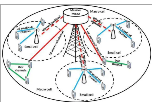
Massive MIMO will play a key technological role to create new spectral and energy-efficient networks [3]. This technology has a great potential to meet the requirements of a next-generation wireless system. In [4], the energy efficiency of massive MIMO and small cells (SC) has been studied. The authors proved that massive MIMO has better energy efficiency when the number of SC is low, while the latter offers better performance when the number of cells is high. However, a globally optimal trade-off between massive MIMO and SC efficiency are hard to achieve due to dynamic network behaviour. A viable solution could be found by converging massive MIMO, SC, device-to-device (D2D) communications into a single cloud-controlled heterogeneous network (HetNet), as shown in Fig. 1.1.
Figura 1.1 – The architecture of a heterogeneous network.
Source provided by the author.
1.1 Channel Estimation Using Reciprocity
One of the big advantages of TDD systems lays on the possibility of estimating the downlink channel based on the assumption of reciprocity. This means that the UL channel matrix within the channel coherence time is a transposed version of the DL one. In this case, the UE sends out the pilots and the BS estimates the UL channel. Then, the BS is able to steer narrow beams towards the UE with a transposed version of the estimated UL channel matrix. The overall process has to be performed within the duration of the channel coherence time, which may not hold in scenarios with moderate or high mobility. This is still true even though, in reality, each UE has RF mixers, filters, and analog-digital converter (ADC)s that make up the equivalent channel model and can potentially break the assumptions on uplink/downlink channel reciprocity [5]. It is important to highlight to the reader that this issue is not uniquely related to massive MIMO, but it has also been studied over the past few years in the context of traditional MIMO systems [5]. However, with massive MIMO systems, a lack of understanding about hardware impairments and a lack of proper modelling persists, and it is still not clear whether they challenge reciprocity or how to mitigate any associated negative effects to keep transmissions reliable. For example, mutual coupling among the BS antennas may not be neglected and may limit massive MIMO performance [6].
1.2 Problem Definition: Channel Estimation Without Reciprocity
Figura 1.2 – The FDD system is composed of two channels: uplink and downlink. The UE estimates the channel by using the pilot sequence sent in the downlink channel, then reports channel estimation in the feedback channel (uplink channel).
Pilot transmission
Channel report Downlink channel
Uplink channel
Source provided by the author.
operate in FDD. In this case, the BS needs to spend communication resources on the DL channel to transmit pilots and needs the UL one to acquire the channel. The CSI is estimated by the UE and then reported to the BS via feedback control channel.
The benefits of using conventional DL channel estimation techniques in traditional MIMO systems that assume small or moderate antenna arrays are well known. However, the amount of time-frequency resources used by the pilot sequence grows with the number of transmit antennas. In the absence of a specific strategy to reduce the sequence length and keep a reliable CSI acquisition, the gains in terms of spectral efficiency of massive MIMO systems tend to disappear [3]. To tackle the DL channel estimation problem, effective pilot transmission methodologies that accurately estimates the CSI with minimal signalling overhead play a crucial role in the success of massive MIMO for FDD systems.
Although traditional MIMO channel estimation techniques require the length of the pilot sequence to be on the same order as the number of BS antennas, optimality is related to the channel covariance matrix [7]. Specifically, by considering the link between BS and UE, the training sequence for each antenna element should be orthogonal. The optimal length corresponds to the number of antennas at the transmitter in i.i.d./Rayleigh channels. However, under spatially correlated channels, and from the assumption that the BS knows the channel correlation matrix perfectly, the authors in [7] and [8] affirm that the optimal training sequence length is equal to the number of dominant eigenvalues. For massive MIMO, it is likely true that the number of eigenvalues is smaller than the number of antennas which means this can be exploited to potentially reduce the pilot overhead.
number of antennas increases. Because of this issue, channel feedback has gained much attention in the massive MIMO research community. Current strategies to tackle the feedback overhead problem try to compress the channel matrix so that the UE sends fewer information to the BS and it can still reconstruct the channel. For instance, non-coherent trellis-coded quantization has been proposed by authors in [9] and the techniques has high compression rates, but at the cost of moderate computation complexity using Viterbi algorithm.
Another perspective are solutions that use sparsity-aware channel estimation techniques. In this case, the UE estimates a sparse channel representation and feeds the non-zero entries back to the BS. Another example of using sparsity is to identify the most representative “channel directions” (transmission angles), which can be fed back to the BS using a few bits [10, 11].
Statistical approaches are also interesting to reduce the system overhead. Using the spatial covariance matrix, the UE and BS can use this information to obtain a reduced version of the massive MIMO channel matrix [12]. This approach will be explained in more detail in this thesis.
This thesis focuses on deriving channel estimators that support applications where the reciprocity does not hold. In this context, the techniques developed in this work relies on two approaches: sparsity and statistics. Such strategies are applied mainly for the pilot and feedback overhead problems. Figure 1.2 summarizes how the system works with DL and UL channels.
1.3 Sparsity and Statistical Approaches to Deal With Overhead
The pilot overhead demanded by channel estimators depends on the number of parameters to infer. In the massive MIMO case, the channel matrix is naturally large which implies the need for many pilots. To reduce the overhead, channel estimators must exploit other representations that lead to a compressed version of the channel.
Usually, the channel matrix is represented with respect to the antenna domain, but such a large matrix is likely to be low-rank. The number of scatters in most environments is usually much less than the number of antennas and generates fewer dominant paths. In this case, the channel can be represented in a compressed version by using a given basis whose choice determines the rate of compression. The optimum basis varies according to the environment characteristics, however, this information is not available in advance for most applications. In such a case, the system imposes a fixed basis up to an error in the estimation process. The approaches considered in this thesis use two frameworks to achieve channel compression: i) compressive sensing (CS) [13, 14] and ii) statistical channel representation [15].
signals which are sparse in the canonical coordinate basis or sparse with respect to some other orthonormal basis. In the context of this thesis, the massive MIMO channel matrix itself is not sparse, but it admits a sparse decomposition.
Second order statistics can also be exploited to obtain channel compression. Environ-ments with only a few scatters lead to a low-rank spatial channel covariance matrix. This means that to accurately represent the instantaneous channel, the estimator only needs a subspace defi-ned by the eigenvectors. Knowing this subspace, the BS smartly designs the pilot sequences [21] and also their length.
In this thesis, each chapter covers a specific aspect of the estimation process between BS and UE, as detailed below
• Chapter 2 (Compressive Sensing for Estimating Narrowband Channels): In this chapter,
we present the fundamental concepts of CS and use them to derive a channel estimator that exploits the flat channel sparsity. Two CS-based estimators are derived, one using a greedy algorithm, called OMP, and one using the ADMM.
• Chapter 3 (Tensor Compressive Sensing for Estimating Frequency Selective Channels): In
this chapter, we investigate channel estimation applied to frequency-selective channels. Such a case involves estimating a collection of matrices, each one corresponding to a given a channel frequency response. To do this, we combine the CS and tensor analysis [22, 23] to jointly estimate the space-frequency channel.
• Chapter 4 (Sparse Channel Estimation for mm-wave Massive MIMO Systems): In this chapter, two problems are investigated: i) one is to optimize the sparse representation of the channel leading to a better channel compression; ii) the other one consist of tracking the angle variations due to the UE mobility.
• Chapter 5 (Statistical Hybrid Beamforming for massive MIMO Channel Estimation): In this chapter, we tackle the problem of estimating the channel using the spatial channel covariance matrix. To exploit such an information, a beamforming technique and a channel estimator are jointly designed to acquire the channel.
Fig. 1.3 summarizes in a block diagram how the thesis is organized.
1.4 List of Contributions
The contributions of this thesis are:
Figura 1.3 – Diagram of the thesis organization.
Beamforming
Sparse Structure
Multidimensional Structure
Statistical Properties Channel
Estimation
Chapter 2 Chapter 3
Chapter 4
Chapter 5
Extension Topic related Massive
MIMO
Source provided by the author.
• A low-complexity channel estimator that jointly estimates a space-frequency massive MIMO channel. This estimator is obtained from the combination between CS and tensor frameworks. To the best of author’s knowledge, there is no estimator in the literature that exploits jointly sparse representation of the channel and still achieves a low-complexity estimator.
• A novel method that includes a new pilot placement on the time-frequency frame to estimate milimeter (mm)-wave channels and deal with the user mobility issues in indoor scenarios. The contribution of the method lays on the case where the UE has multiple antennas and the system uses an OFDM modulation .
In terms of scientific production, this thesis has
• Journal
– ARAÚJO, D.C., MAKSYMYUK, T., de ALMEIDA, A.L.F, MACIEL, T.F ; MOTA, J.C.M; “Massive MIMO: Survey and Future Research Topics", IET Communications, to appear, 2016.
• Conferences
– ARAUJO, D. C. ; de ALMEIDA, A. L. F. ; MOTA, João C M ; HUI, D. “Esti-mation of Very Large MIMO Channels Using Compressed Sensing". In: Simpósio Brasileiro de Telecomunicações, 2013, Fortaleza. Anais do Simpósio Brasileiro de Telecomunicações, 2013
– ARAUJO, D. C. , de ALMEIDA, André L.F., AXNAS, J. MOTA, J.C.M. , “Chan-nel Estimation for Millimeter-Wave Very Large MIMO", . In: European Signal Processing Conference (EUSIPCO), Lisbon, 2014.
– D. C. Araújo, A. L. F. de Almeida and J. C. M. Mota, “Compressive sensing based channel estimation for massive MIMO systems with planar arrays,"Computational Advances in Multi-Sensor Adaptive Processing (CAMSAP), 2015 IEEE 6th Internati-onal Workshop on, Cancun, 2015, pp. 413-416. doi: 10.1109/CAMSAP.2015.7383824 – ARAÚJO, D.C., KARIPIDIS, E., de ALMEIDA, A. L. F., MOTA, J. C. M . “Impro-ving Spectral Efficiency in Large-Array FDD Systems with Hybrid Beamforming", Proc. of IEEE 9th Sensor Array and Multichannel Signal Processing Workshop (SAM 2016), Rio de Janeiro, 2016.
– ARAÚJO, D.C., KARIPIDIS, E., de ALMEIDA, A. L. F., MOTA, J. C. M . “Hybrid Beamforming Design Using Finite-Resolution Phase-Shifters for Frequency Selective Massive MIMO Channels", submitted on ICASSP 2017.
• Patent
– SUNDSTROM, L. and Hui, D. and Reial, A. and ARAUJO, D.,“Antenna Beam Control”, Reference WO 2015135987 A1.
This work was developed in the context of UFC/ERICSSON Research partnership. The thesis is also product of two research projects over the last 4 years:
• UFC.34Advanced MIMO Transceivers and Matrix Decompositions for Wireless Systems, August/2012 - July/2014;
How to Read This Thesis
2 COMPRESSIVE SENSING FOR ESTIMATING NARROWBAND CHANNELS
Abstract:
In this chapter, the problem of estimating single-user massive MIMO channels using DL pilots is investigated. In this context, the number of DL pilots tends to increase as the number of antennas scales up. Assuming the channel is flat, the estimator exploits the inherent channel structure which reduces the number of estiamted parameters . This occurs because the channel has a sparse representation in the spatial domain. To derive a sparsity-based estimator, the CS framework is applied. With this approach, we derive three methods: one uses a greedy algorithm, the second uses Lasso criterion, and the third implements the Lasso criterion but in a distributed fashion. The motivation to use a distributed solution comes from the increased computational complexity demanded by the two first methods. The results show that it is possible to reduce the pilot sequence and achieve precise channel estimation by exploiting the channel sparsity. Moreover, the Lasso criterion outperforms the greedy algorithm mainly for low SNR, and its distributed version has a negligible loss Normalized Mean Square Error (NMSE) with respect to the centralized solution. The conclusions and open questions are presented in the end of this chapter.
2.1 Introduction
The promised benefits of massive MIMO systems are strongly dependent on the quality of the CSI available at the receiver and/or transmitter. Conventional channel estimation approaches rely on training sequences [1, 24, 25] and most of them use a least square (LS) approach to estimate the channel. However, this technique requires that the length of the training sequences must be at least equal to the number of transmit antennas which demands precious communication resources and energy.
found many different applications such as image processing, radar, sub-Nyquist sampling, just to mention a few [14, 17, 20].
In the channel estimation problem, CS finds many attractive scenarios for its application as for example ultrawideband systems, underwater communication scenarios, mm-wave channels, just to mention a few ones [26–28]. The cited examples have channels that admit a sparse representation on the delay domain, i.e. the power delay profile has very few representative taps. This feature is exploited by the channel estimator to reduce the length of the pilot sequences. In [29], the case of interest is the multi-user scenario where the number of antennas at the BS grows large and the number of UE as well. To achieve channel estimation without vanishing the communication resources, the estimator relies on the channel sparsity to reduce the necessary overhead to estimate such a large channel. This strategy overcomes other techniques that use a LS criterion.
Even though the authors in [29] provide a great contribution in proposing a sparse channel estimator, the solution only has application in crowd environments. The technique relies on the fact that both BS antennas and the number of UEs grow largely, this situation is envisaged as a possible application in 5G [30]. However, there is room for working with single-user scenario. In this case, the BS serves only one user per resource, which means that the multiplexing capabilities of the large array are not enjoyed by the UEs, but rather the array gain. Single-user solutions still find many applications on currently wireless standard systems as for instance, to overcome some coverage limitation issues. Furthermore, the development of receivers with multiples antennas is also considered. They can become very popular with the use of mm-waves because the higher the frequency is, the more the antenna array can be packed [31].
One bottleneck that arises when assuming multiple antennas at the UE is the hardware complexity and the amount of signals to process. Each antenna element at the UE collects a signal which is then sampled and processed in baseband. However, the more antennas are employed, the more processing capabilities to treat the signal are required. In the channel estimation problem, CS helps by reducing the pilot sequence length, and consequently reduces the number of samples to be processed. However, we can further reduce the hardware complexity by using a distributed processing in the baseband part [32]. Specifically, we employ a set of channel estimators that handle small portions of the training sequence. Each estimate is informed in a central node that combines the estimates and report back to each estimator. Such an architecture of an estimator has not been considered yet.
This chapter shows a pilot-assisted technique based on CS theory for channel estimation. To obtain an approximate sparse representation, we consider that angles of departure and arrival are modelled by the Fourier basis. We provide three strategies:
algorithm calculates the channel projections onto the directions.
• The second solution is derived from the Lasso problem [14, 33]. This formulation tries to find the sparsest solution taking into account the power of the noise.
• The third solution introduces a distributed implementation of the Lasso solution. This
becomes an attractive solution for those receivers with limited processing capacity.
All the three methods are compared with the CRLB. From this development, we verified that the set of pilot sequences that leads to a Grassmanian real matrix are necessarily the optimum ones. To the best of author’s knowledge, this results have not been addressed yet in the literature.
2.2 Compressive Sensing Background
In recent years, CS has become very popular in many areas such as mathematics, compu-ter science and electrical engineering just to mention a few. The key idea of CS is to recover a sparse signal from very few linear measurements. The theory shows that it is possible to recover N parameters withM < N measurements if the estimator uses a suitable basis that leads to a sparse representation of the data. Thus, the theory offers a framework for simultaneous sensing and compression of finite-dimensional vectors. A lot of results and theorems can be found in the literature, and from this broad literature, we present in this section only the most fundamental concepts and just those that will be used in this thesis [13, 14, 16, 34].
2.2.1 Undetermined Linear Systems
Consider the matrixΨ∈CM×N withM < N that defines a undetermined linear system Ψx=y. This configures a system with less equations than variables, and it has either no solution
or infinite solutions. The first case happens when the vectoryis not in the span of the matrixΨ.
The second case happens otherwise. To avoid the situation where we have no solution, let us assume thatΨis full rank.
In many areas, it is common to face problems that lead to undetermined linear systems. For instance, we refer to the problem in [14]. The authors investigate the reconstruction of a waveform assuming fewer measurements than the minimum to meet the Nyquist criterion. Even though this classical condition is not achieved, the signal is completely recovered by exploiting the knowledge of signal basis representation. Using this information the authors obtain a compressed representation of the signal and which makes it possible to recover the signal even at sub-Nyquist rates.
2.2.2 General Problem
Definition 1 Letθ∈CN, if there existK < N nonzero entries, then it is aK-sparse vector.
In practice, the vector to be estimated is not always sparse. If this happens, then the estimator has to use a basis that leads the signal of interest into a sparse representation. Thus, consider a given signalx∈CN as the signal of interest and letΦ∈CN×N be an orthonormal basis such
thatθ=ΦHxis aK-sparse vector. The matrixΦcompressesxif the codebookΦsparsifiesx.
An example where this concept can be applied refers to the communication channel models. In practice, the channels are composed by scatters that define the channel impulse response. If it has only few scatters, then the channel is likely to be sparse. A model that we hardly can rely on sparsity is the estimation of i.i.d channels. In this situation, the problem is unstructured and does not admit a sparse representation in the spatial domain.
The acquisition ofxis a process that is modeled as a linear transformation, where a
measurement matrixΨis applied overx. The signal observed then is represented asy=Ψx CM. The number of elementsM inyrefers to the number of measurements that are taken from
the vectorx. The acquired signal can be written asy=Ψx =ΨΦθ[13, 16, 35].
The goal of the CS formulation is to find the sparsest solutionθ such that it attains
y=ΨΦθ. Thus, the optimization problem can be stated as
argmin
θ k θk
0
s.t. y=ΨΦθ, (2.1)
wherek.k0 stands for thel0-norm. This norm is of interest to this problem because it returns the
number of non-zero entries ofθ. However, the problem (2.1) is non-convex and also NP-hard due to thek.k0. Therefore, to have a tractable problem, it is modified by changing thel0-norm to
another one that achieves convexity. Thek.kpoperator is non-convex for the range0< p <1,
as can be seen in Figure 2.1. Therefore, a reasonable heuristic for relaxing (2.1) consists of approximatingk.k0 tok.k1 representation. Thus, the new problem is
argmin
θ k θk
1
s.t. y=ΨΦθ. (2.2)
Thel1-minimization approach is now a convex problem and can be solved by using linear
pro-gramming if it is real, or second order cone propro-gramming if it is complex [13]. The assumptions usually considered when relaxing this problem are:
Figura 2.1 – Plot of a functionkθkp∀p∈[0,1], whereθ ∈R.
(a)p= 0
−1 −0.8 −0.6 −0.4 −0.2 0 0.2 0.4 0.6 0.8 1
−1
−0.8
−0.6
−0.4
−0.2 0 0.2 0.4 0.6 0.8 1
θ1 θ2
(b)p= 0.4
−1 −0.8 −0.6 −0.4 −0.2 0 0.2 0.4 0.6 0.8 1
−1
−0.8
−0.6
−0.4
−0.2 0 0.2 0.4 0.6 0.8 1
θ1 θ2
(c)p= 0.8
−1 −0.8 −0.6 −0.4 −0.2 0 0.2 0.4 0.6 0.8 1
−1
−0.8
−0.6
−0.4
−0.2 0 0.2 0.4 0.6 0.8 1
θ1 θ2
(d)p= 1
−1 −0.8 −0.6 −0.4 −0.2 0 0.2 0.4 0.6 0.8 1
−1
−0.8
−0.6
−0.4
−0.2 0 0.2 0.4 0.6 0.8 1
θ1 θ2
Source: Provided by the author.
2. The sparsity measure is very sensitive to small entries inθ. A good approach consists in defining a threshold to eliminate such values.
2.2.3 Uniqueness Conditions for the Compressive Sensing Problem
A key property to understand the conditions of uniqueness is thesparkof the matrix
Υ= ΨΦ. This property provides a way of describing the null-space ofΥusing thel0-norm.
This concept is enunciated with the following definition.
Definition 2 The operatorspark{Υ}is the smallest number of columns fromΥthat are linearly dependent.
Note that there is a resemblance between the definition of rank and spark. From linear algebra, the rank is defined as the largest number of columns inΥthat are linearly independent.
to perform an exhaustive search over all the possible subsets formed by the columns ofΥ. This
is more complex than rank calculation [35].
Apart from the complexity issue, the spark is a powerful definition to reveal the uni-queness ofθ. The vectors in the null-space ofΥ, i.e.Υθ =0, must combine linearly at least spark{Υ}dependent columns ofΥ. Using the spark definition, the uniqueness condition is
ensured by the following theorem:
Theorem 1 If a set of equations is represented as a linear system in the form Υθ = y, its sparsest solution obeyskθk
0 < spark{Υ}/2.
To understand Theorem 1, consider two vectorsθ1andθ2 as null-space elements ofΥand the differenceθ1−θ2 must also be in the null-space. Using the definition of spark, we get
kθ1k
0+kθ2k0 ≥ kθ1−θ2k0 ≥spark{Υ}. (2.3)
This inequality shows that the number of non-zero entries ofθ1−θ2 cannot exceed the sum of the non-zero entries of each vector θ1 and θ2, which follows from the triangle inequality. From this observation, and assuming kθ1k
0 < spark{Υ}/2, it is possible to conclude that
kθ2k
0 > spark{Υ}/2.
Becausespark{Υ}is very difficult to evaluate, its use in uniqueness analysis is very
complicated. An alternative is to exploit the mutual coherence concept which is presented in the following definition.
Definition 3 The mutual-coherence of a given matrixΥis the largest absolute inner product between all the different columns ofΥ. Denoting theith column ofΥas[Υ]i, the mathematical formulation is given by
µ(Υ) = max
1≤i,j≤N,i6=j
|[Υ]Hi [Υ]j| k[Υ]ik2
[Υ]j 2
. (2.4)
Note that for the orthogonal matrix, the mutual coherence is zero. For the case of interest, M < N,µ(Υ)is positive, and the smaller isµ(Υ), the closer the estimator performance is to
the case where orthogonal matrices are used.
Mutual coherence is far easier to compute than the spark. It is then interesting to establish a relationship between spark and mutual coherence. Following, it can be stated [35]
spark{Υ} ≥1 + 1
µ(Υ). (2.5)
Theorem 2 The sparsest solution of a linear systemΥθ =yobeys the relationship
kθk
0 <
1 2 1 +
1
µ(Υ)
!
. (2.6)
Theorems 1 and 2 are similar, but they carry different assumptions. The first one, which relates spark and uniqueness, is more powerful than the second one, which uses the mutual coherence to guarantee uniqueness. The mutual coherence is lower bounded by √1
M, thuskθk0 in Theorem
2 cannot be larger than√M /2. However, the spark can be as larger asM. This gives a bound of M/2.
2.3 Narrowband Structured Channel Model
Consider a MIMO system withNTantennas at the transmitter andNRantennas at the
receiver. Assume that the receiver does not have any knowledge about the communication channel. Thus, the receiver needs to estimate the channel using, e.g. a known training sequence sent by the transmitter. The received training signal is denoted by
Y=SH+Z. (2.7)
The matrixS ∈ CT×NT contains the training sequences sent by each one of the N
T transmit
antennas, where T denotes the length of the training sequence, H ∈ CNT×NR is the channel matrix andZis the additive white Gaussian noise matrix whose entries have varianceN0/2, and
the matrixY∈CT×NR defines the received signal.
It is a common practice in the literature to use i.i.d entries for modelling the MIMO channel. However, this assumption leads us to overestimate the spatial degrees of freedom. This is especially true for massive MIMO channels where the number of transmit/receive antennas may be significantly higher than the degrees of freedom provided by the channel [36]. Thus, the i.i.d. case is not considered hereafter but instead a structured channel model.
In [36], a stochastic MIMO channel model, inspired by the Kronecker model and virtual channel model, was proposed. Combining the advantages of both models, the so-called Wei-chselberger’s model shows enhanced capabilities to model the spatial structure of the channel. However, the price for achieving a more accurate channel representation is the knowledge of the transmit and receive one-side correlation matrices. Such matrices are defined as
RR = EnHHHo=UrΛrUrH,
RT = E
n
HHHoT =UtΛtUtH,
(2.8)
where, the matricesUr(resp.Ut) andΛr(resp.Λt) are the receive (resp. transmit) eigenvector
In [36], Weichselberger proposes the following channel decomposition model
H=Ut(Ω⊙G)UrH (2.9)
whereΩis a positive and real-valued matrix, being equal to the square-root of the power coupling
between transmit and receive eigenmodes,Ghas i.i.d entries that accounts for the channel fading,
and⊙denotes the Hadamard product. A full-rank matrixΩmeans a scattering-rich environment
with maximum diversity. In this situation, model (2.9) is equivalent to the Kronecker model. In [36, 37], the authors show that if the number of antennas goes to infinity, the discrete Fourier transmform (DFT) matrix is asymptotically equal to the matrix of eigenvectors.
2.4 Compressive Sensing to Massive MIMO Channel Estimation
Channel estimation using a LS criterion applies the pseudoinverse ofSover the received
signal. However, such an operation is only possible ifT ≥NT. This imposes a practical issue that
decreases the spectral efficiency, onceNT is very large. The desirable situation is thatT ≤NT,
but this leads to a system with less equations than variables, and, consequently infinite solutions. On the other hand, using compressed sensing, the receiver can estimate such a large channel withT ≤NT. First, it is necessary to find an appropriate codebook (also known as “dictionary”) Φto obtain a sparse representation ofH.
Consider Eq. (2.7) and the property vec{ABC} = CT ⊗Avec{B}, the received
signalYas
vec{Y} =vec{SH}+vec{Z}
=ITNR ⊗Sh+vec{Z}, (2.10) whereh=. vec{H} ∈CNTNR.Substituting (2.9) into (2.10), we derive the expression
vec{Y} =ITNR⊗S(U∗r ⊗Ut)vec{(Ω⊙G)}+vec{Z}. (2.11)
Then, we define
y =. vec{Y} ∈ CT NR, (2.12)
z =. vec{Z} ∈ CT NR, (2.13)
Ψ =. ITNR ⊗S ∈ CT NR×NTNR, (2.14)
Φ = (. U∗r ⊗Ut) ∈ CNTNR×NTNR, (2.15)
θ =. vec{(Ω⊙G)} ∈CNTNR×NTNR, (2.16) which allows one to compactly rewrite (2.10) as
Note that in this model, the measurement matrix Ψ depends on the set of pilot sequences
contained inS. Their length and the number of antennas at the receiver correspond to the total
number of measurements that the receiver has access. This number can be reduced if the channel vector hadmits a sparse representation. This is because we can use CS theory to reduce the
lengthT of the pilot sequences.
The channel sparsity is achieved using the dictionaryΦto modelh. This representation
is obtained from the transmit-receive spatial basesUtandUrrespectively. These matrices model
statically the paths that compose the channel. The coupling matrixΩdefines the power associated
with the scatters and how the paths of the transmit and receive sides connect among themselves. If we consider a full matrixΩ, it means that all the scatters communicate with each other and the
model reduces to Kronecker channel model [36]. However, it is known from the literature [36] that the consideration creates clusters that do not exist, i.e. it overestimates the richness of the channel [38]. Therefore, it is correct to assume thatΩis sparse.
The sparsity of the model depends on the basis adopted to represent the channel. For the same channel vec{H}, there are more than one sparse representation and they may lead to
different sparse representations. The compression provided by the eigenvectors in the model (2.9) can only be achieved if the receiver knows such bases. These orthonormal matrices are obtained from the covariance matrices of the transmit and receive side which means that the receiver needs to acquire such an information. The acquisition demands an extra overhead before the estimation of the instantaneous channel, but Ut and Ur are long-term information and remain constant
over many time instants. In the case, if we have large arrays at both, transmitter and receiver, these matrices tend to be the DFT. The advantage of this result is that the covariance matrix acquisition can be avoided. Thus, it is possible to derive a sparsity-based channel estimation technique assuming the DFT approximation to reduce the pilot sequence.
2.5 Cramer-Rao Bound Discussion For Estimating Sparse Channels
The CRLB provides a benchmark to analyse how good is the accuracy of a given channel estimator. If it attains the CRLB in linear estimation problems, the solution is equivalent to the minimum variance and unbiased (MVU) estimator [15]. This type of estimator applied to the problem in (2.17) must be capable of extracting the sparse channelθ. The accuracy of such an estimator is compared with the benchmark provided by the CRLB, which makes it possible to obtain insights with respect of the estimator accuracy.
In (2.17), the vectorized representation of the received signal contains a white noisez.
Each sample of noise follows the complex multivariate Gaussian distribution and the samples are idealistically uncorrelated. In practice, correlated noise is present because of interference sources. However, this case is not taken into account in this thesis.
an estimatorθˆ, so that it applies a linear transformation onto the received samples, i.e.ˆθ=g(y), whereg(.)is some function. To determine good estimators, it is important to firstly establish a
statistical model for the measurements, so that it describes the randomness due to the presence of noise. The characterization of y by the probability density function (PDF) p(y;θ) and parametrizing the PDF with the unknown parameterθ become a fundamental prerequisite to obtain the CRLB. With this model, a class of PDFs is generated, where each of them differs according to the values ofθ.
Assuming the PDF of the noise, Eq. (2.17) are considered, and that the sparsitykθk
0 =K
is known a priori, the PDF of the received signal can be expressed as
p(y;θK,θ∗
K) =
1
(2πσ2)T NR/2 exp
(y−ΨΦKθK)H(y−ΨΦKθK)
2σ2 , (2.18)
whereσ2 is the noise variance,θ
K is a vector that contains only theK non-zero entries ofθ,
andΦK is the range space ofΦ. For convenience, we decide to express the PDF as a function of
θ andθ∗as if they were different variables. This type of assumption was already used in other works as for instance in [39].
The multivariate CRLB gives a bound for any unbiased estimatorθˆ in function of the
Fisher information matrix
CCRLB−I(θK,θ∗
K)−1 ≥0K×K, (2.19)
where the Fisher information matrix is given by
I(θK,θ∗
K) =−E
(
∂lnp(y;θK,θ∗
K)
∂θH K∂θTK
)
. (2.20)
To calculate this matrix, the first derivative with respect toθH of the functionlnp(y;θK,θ∗
K)is
obtained
∂lnp(y;θk,θ∗
k)
∂θH
k
= 1
2σ2
M
X
m=1
y[m]−[Ψ]Hm[Φ]kΦH[Ψ]m.
Then, the second derivative is obtained
∂2lnp(y;θ
k,θ∗k)
∂θH k∂θTk
=− 1 2σ2Φ
HΨΨHΦ.
From the second derivative, the Fisher information matrix is given by
I(θK,θ∗
K) = 1 2σ2Φ
HΨΨHΦ. (2.21)
Note that the fisher information matrix defined in (2.21) is composed by the inner product of
Υ=ΨΦ. This means that the off-diagonal elements can be described as
From Definition 3, it is possible to conclude that the matrixI(θK,θ∗
K)gives also information
about the mutual coherence, which is the highest value among all the off-diagonal entries. Besides this, the pilot design also plays an important role in the estimation process. Note that, if the system was able to employ orthogonal pilots, the Fisher information matrix would be diagonal. However, because of overhead issues, the length of the training sequences is shorter than the total number of antennas, which makes it impossible to achieve orthogonality in this case. One way to reduce the loss of performance compared with the orthogonal case consists of designing pilot sequences that have good properties of cross-correlation. It can be measured from the off-diagonal entries of the matrixΨΨH, where the maximum value among all the entries
must be minimized. To achieve such a condition, the mutual-coherence of the pilot sequences must achieve their minimum value.
From CS, ifΨis a full-rank matrix, its mutual coherence is bounded as shown in [35].
Applying this result to the problem, the minimum value is given by
µ(Ψ) ≥ s
NTNR−T NR
T NR(NTNR−1)
≥ s
NT−T
T (NT−1). (2.23)
The equality is only achieved for a family of matrices called Grassmannian [35]. For these matrices, the angles between each pair of columns is the same, and is also the smallest possible. This type of matrix is extremely attractive to produce pilot sequences. However, the problem is to obtain such a Grassmannian matrices. They are usually very difficult to be obtained, but heuristics can be used to achieve approximations as shown in [35].
2.6 Channel Estimators and Receiver Structures
The use of downlink pilots in massive MIMO tends to limit the system spectral efficiency. Classical estimators as LS estimators achieve the minimum error upon the use of orthogonal sequences. However, to achieve this orthogonality the length of such sequences is at least equal to the number of antennas. This indeed demands a lot of communication resources in massive MIMO and consequently reduces the promised spectral efficiency gains. There is a need for techniques that achieve good accuracy, but demanding fewer pilots.
2.6.1 Greedy Channel Estimation Method
Let us consider in a first moment a scenario without noise so that we can study the problem. Suppose that the matrixΥhasspark{Υ}>2, and the solution for the problem
θ =argminkθk
0 s.t.y=Υθ, (2.24)
iskθk
0 = 1. This means that the vector of measurementsyhas one scalar that multiplies one
of the columns of the matrixΥ, and this solution is known to be unique [13]. It is possible to
identify this column by applying NTNR tests, one for each column ofΥ. Thenth test can be
performed by minimizing the error
e(n) =k[Υ]nωn−yk22. (2.25)
This leads to the solution
ωn′ = [Υ] H n y
k[Υ]nk2 2
. (2.26)
Substituting the equation (2.26) into (2.25) the error expression becomes
e(n) =k[Υ]n [Υ] H n y
k[Υ]nk2 2 −
yk22
=kyk22+ [Υ] H n y
k[Υ]nk2 2
!2
k[Υ]nk2 2−
[Υ]Hn y
k[Υ]nk2 2
!∗
[Υ]Hn y− [Υ]
H n y
k[Υ]nk2 2
!
yH[Υ]n
=kyk22+
[Υ]Hn y2
k[Υ]nk2 2 −
[Υ]Hn y
k[Υ]nk2 2
!∗
[Υ]Hn y− [Υ]
H n y
k[Υ]nk2 2
!
yH[Υ]n
=kyk22− [Υ]
H n y
k[Υ]nk2 2
!∗
[Υ]Hn y (2.27)
Ife(n) = 0in (2.27), the non-zero entry ofθwas found. Thus, the test to identify the entry of interest is
kyk22− [Υ]
H n y
k[Υ]nk2 2
!∗
[Υ]Hn y = 0
[Υ]Hn y
k[Υ]nk2 2
!∗
[Υ]Hn y =kyk22
|[Υ]Hn y|2 =kyk22k[Υ]nk2
2. (2.28)
The expression (2.28) shows that ifyand[Υ]nare parallel,nis the non-zero entry ofθ. The search procedure in this case takes a number of operations on the order ofO(T NTNR)flops.
Consider nowspark{Υ}>2K0andkθk0 =K0. The vectoryis a linear combination
of at mostK0 columns ofΥ. Using the same solution, the optimum approach is to test all the
N TNR K0
possible combination of columns fromΥ. The number of operations in this situation is
ONTK0NRK0T K02
Figura 2.2 – Centralized channel estimation solution using greedy algorithm.
ADC
ADC
Source: Provided by the author.
A greedy algorithm avoids such combinatorial solution and evaluates a series of locally optimal single-term updates. From these local problems, the algorithm constructs iteratively a sparse vectorθK by using the rule in (2.28). The columns corresponding to the non-zero entries ofθreduces maximally the residual error in approximatingy. Using the column ofΥobtained from each iteration, the residual error is evaluated and if it falls below a predefined threshold, the algorithm stops. The pseudocode is shown the Table 1.
The implementation of the algorithm consists of collecting the training signal after the analog-digital conversion, followed by an operation that performs the vectorization of the samples. This vector is the input to the algorithm described in Table 1.
Although the OMP algorithm saves computational processing by avoiding exhaustive search through allN
TNR K0
possible combination of columns from Υ, the search procedure of
finding the strongest components can also lead to a lot operations. The number of multiplications is O
NTK0NRK0T K02
and because we have a massive array the implementation of such an algorithm can be prohibitive on devices with limited processing capabilities. The block diagram of the receiver is shown in Fig.??
2.6.2 Distributed Linear Regression for Sparse Channels Using ADMM
Let us consider the problem ofl1 regression known as Lasso [35] which is stated as
min
θ (1/2)kΨΦ
θ−yk2
2 +βkθk1, (2.29)

![Figura 2.1 – Plot of a function k θ k p ∀ p ∈ [0, 1], where θ ∈ R . (a) p = 0 −1 −0.8 −0.6 −0.4 −0.2 0 0.2 0.4 0.6 0.8 1−1−0.8−0.6−0.4−0.200.20.40.60.81 θ 1θ2 (b) p = 0](https://thumb-eu.123doks.com/thumbv2/123dok_br/15349566.561777/29.892.170.768.160.670/figura-plot-function-θ-θ-r-θ-θ.webp)