Internal Model Control of A Class of Continuous Linear Underactuated Systems

Internal Model Control of A Class of Continuous

Linear Underactuated Systems

Asma Mezzi

Tunis El Manar University,

Automatic Control Research Laboratory, LA.R.A, National Engineering School of Tunis (ENIT),

BP 37, Le Belvédère, 1002 Tunis, Tunisia

Dhaou Soudani

Tunis El Manar University,

Automatic Control Research Laboratory, LA.R.A, National Engineering School of Tunis (ENIT),

BP 37, Le Belvédère, 1002 Tunis, Tunisia

Abstract—This paper presents an Internal Model Control (IMC) structure designed for a class of continuous linear underactuated systems. The study treats the case of Minimum Phase (MP) systems and those whose zero dynamics are not necessarily stable. The proposed IMC structure is based on a specific controller which is obtained by the realization of an approximate inverse of the model plant. It is shown that, using such IMC structure, it is possible to remedy the problem of system underactuation and Non-Minimum Phase (NMP) behavior. The case of non-zero initial conditions and imperfect modeling are also presented and model parameters effects on the system evolution are discussed. Simulated examples are presented to prove the effectiveness of the proposed control method to ensure set-point tracking, stability and disturbance rejection.

Keywords—Internal Model Control; continuous linear underactuated systems; specific controller; minimum phase systems; non-minimum phase behavior; non-zero initial conditions; model parameters effects; set-point tracking; stability; disturbance rejection

I. INTRODUCTION

Multivariable underactuated systems, i.e., systems having fewer control inputs than degrees of freedom, are widely used in industry. Aircraft, helicopters, underwater vehicles, surface vessels, mobile systems and many of today’s walking and underwater robots are some examples of underactuated systems. They are used for reducing cost, weight or energy consumption. Some other advantages of underactuated systems include tolerance for actuators failure and less damage while hitting an object. The dynamics of some underactuated systems may contain NMP behavior which causes much more challenging control problems.

Over the last years, research in the field of underactuated control systems have led to significant advance and several control methodologies have been proposed. In order to contribute to this research area, we propose to extend an interesting control approach (called IMC) to a class of continuous linear underactuated systems.

The IMC is considered as one of the most powerful control approaches thanks to its robustness and simplicity. In 1982, it was defined for Single-Input Single-Output systems (SISO) by Morari and Garcia and extended to Multi-Input Multi-Output (MIMO) ones in 1985 [3, 8]. Since then, several structures of continuous-time, discrete-time, linear and non-linear IMC have

been proposed [1, 2, 4, 5, 6, 7]. These studies have covered many classes of SISO systems and MIMO fully-actuated ones where the number of control inputs is equal to that of the outputs. Among the proposed IMC approaches, we are mostly interested in the IMC structure proposed in [7]. The specificity of this IMC structure resides in the use of a special controller which is an approximate inverse of the model plant. The use of this controller ensures a high level of robustness and system performance reservation even in the case of NMP systems and those with a time-delay [1, 5]. A number of studies of this IMC structure have been applied to both linear and non-linear SISO systems [1, 6, 7] as well as multivariable fully-actuated ones [2, 4]. The obtained results are very satisfactory which led us to extend the approach to a class of continuous linear multivariable underactuated systems.

An internal model controller of a class of continuous linear multivariable underactuated systems is presented in this paper. Cases of linear MP and NMP underactuated systems are studied. Simulation results confirm the effectiveness of the approach to ensure stability, accuracy and system performance reservation in spite of the presence of external disturbances, unstable zeros and non-zero initial conditions. The influence of the model parameters on the system behavior is also discussed.

The rest of this paper is divided into three sections. Firstly, the proposed approach is described beginning with a review of the IMC basic structure which was designed for linear multivariable fully-actuated systems, followed by the explanation of the encountered basic problems and the proposed solutions. Secondly, two illustrative examples, in which our proposed IMC structure is applied to cases of MP and NMP linear underactuated systems, are presented. Thirdly, the influence of non-zero initial conditions on the system evolution is treated and finally, effects of the model parameters are discussed.

II. THE PROPOSED APPROACH

A. The basic IMC structure

The IMC structure has several advantages. For example, it guarantees the closed loop system stability, anticipates constraint violations and allows for corrective actions. Also, a perfect set-point satisfaction can be achieved despite the presence of external disturbances.

Fig. 1. IMC basic structure (MIMO fully-actuated systems)

The controller C is the inverse of the chosen model if it is realizable. Its structure and parameters are known a priori which simplifies the process of finding a suitable approximation for a practical implementation.

In the case of multivariable fully-actuated systems, n is the number of the system inputs and outputs, r is a reference signal of a dimension (n 1), y is the process output vector of a dimension (n 1), ym is the model output vector of a

dimension (n 1), v is a disturbance signal affecting the system and uc is the control input signal of a dimension (n 1)

[2, 4]. As shown in Fig. 1, the signal uc, which is generated by

the controller C, is applied to the plant and the model M alike. The signal d represents the calculated difference between the process output signal y and the model output signal ym. It also

represents the disturbance effect and the modeling errors, as shown in (1).

e=r-d = r-((G(s) - M(s))u(s) +v(s)) (1) The signal d is then compared to the reference signal r to generate the controller input signal e.

In the case of linear multivariable fully-actuated systems, the process and its model can be presented by their square transfer matrices of dimension (n n) or their space state representations [2, 4].

The internal model control structure is stable if and only if the process, the model M and the controller C are stable in the open loop. In other words, the characteristic polynomials of the plant, the model and the controller state matrices should verify the Routh-Hurwitz stability criterion. The controller synthesis and stability conditions will be discussed in more details in the following section.

B. Main problems

The synthesis of an IMC controller that is equal to the inverse of the model expression is essential in order to ensure perfect set-point tracking. This inversion represents the basic problem of the IMC approach. In fact, the realization of the direct model inverse is difficult or not possible for most physical systems. This difficulty is due to the denominator order on the model expression, which is usually greater than the numerator one, or the presence of unstable zeros or/and

time delay. The direct model inversion is also impossible in the case of underactuated plants. In fact, the model must provide an accurate description of the process dynamics and characteristics. Therefore, the model expression must be very close to that of the plant. For underactuated systems, the number of control inputs is equal to m, the number of outputs is equal to n, and the transfer matrix of the plant is of a dimension (n m) making it a non-square matrix. In this case, the model cannot be invertible. This represents the major problem encountered.

In addition to the system underactuation, the presence of NMP dynamics complicates the system control and makes it much more challenging. In fact, an NMP system, i.e., a system with zeros in the Right Half of the Plane (RHP), is presented by an NMP model. As explained previously, the controller which must be stable is an inverse of the model expression. This inversion may generate an unstable controller. To remedy these problems, we propose firstly to modify the IMC basic structure so that it becomes applicable to underactuated systems. Secondly, we design an approximate inverse of the model plant which is inspired of studies of [1, 7] in the case of SISO systems, and those of [2, 4] in the case of multivariable fully-actuated systems. This proposed controller represents a remedy for NMP systems.

These proposed solutions will be detailed in the following section. The system and model transfer matrix representations will be considered in order to simplify the study and the proposed approach explanation.

C. Proposed IMC structure for linear underactuated systems 1) The proposed IMC design

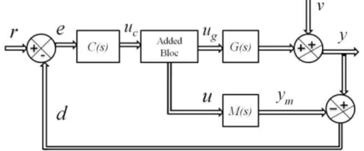
Underactuated systems are systems with more outputs than control inputs. Therefore, the transfer matrix of a linear underactuated system cannot be square. As mentioned in the previous section, on the one hand, the model M must be chosen as very close to the process G; and on the other hand, the controller C is an approximate inverse of the model which requires a square transfer matrix M. The suggested solution consists of utilisating a square model then eliminating the excess control inputs which are applied to the system. This procedure has led to the proposed IMC structure as presented in Fig. 2 [9, 10].

Fig. 2. IMC structure for linear multivariable underactuated systems

11 1

1

m

n nm

G (s)

G (s)

G(s)

G (s)

G (s)









 











(2)

The matrix M(s) must be chosen close to G(s), but as explained previously, the inversion problem requires that the matrix M(s) must be square [2]. To solve this problem, a number of (n (n m)) transfer functions are added to the matrix M(s) in order to make it a square matrix having a dimension of (n n) [9, 10]. Therefore, the IMC structure designed for multivariable fully-actuated systems (where (m = n)) can be applied. The (n (n m)) added functions can be chosen as first-order transfer functions which verify the Routh- Hurwitz stability criterion in order to simplify the study and avoid inversion problems [9, 10]. The obtained matrix M is expressed by (3).

11 1 1 1 1

1 1

added transfer Initial transfer

functions functions

(n x (n-m)) (n x m)

m m n

n nm nm nn

M ( s )

M ( s ) M

( s )

M ( s )

M( s )

M ( s )

M ( s ) M

( s )

M ( s )

 









 











(3)

Secondly, the IMC structure designed for multivariable fully-actuated systems (proposed in [2]) is modified in order to eliminate the (n m) excess control inputs. To do so, a bloc is added to the basic IMC structure as shown in Fig. 2 [9, 10]. It is used to eliminate the (n m) excess control inputs acting on the process G by the use of usual arithmetic operators, as shown in Fig. 3.

Fig. 3. The added bloc

Where ug is the vector of the m control inputs acting on the

process G ;

u

e

=[

u

e1

…

u

ef

]

T is the vector of the (n m) excess control

inputs ;

u

f

=[

u

f1

…

u

ff

]

T is the vector of the (n m) eliminated

excess control inputs.

uf is the control input vector acting on the (n (n m))

added transfer functions of the model M and u is the control input vector acting on the model M.

The control inputs vectors u and ug, the signals d and e, and

the system output vector y are given respectively by these following expressions and equations.









1 1

1

0

0

T

m m n

Eliminated excess control inputs Control inputs acting

((n-m) x 1) on the plant

( m x 1 )

T

g m

u

u

...

u

u

...

u

u

u

...

u











(4)

( ) ( ) g ( ) ( )

d s G s u M s uv s

(5)

( )

( )

( ) ( ( )

_g

( )

( ))

d s

e s



r s



G s u



M s u



v s

(6)

1 2

( )

( )

( )

g g g

u

s



u

s



u

s

(7) where









1 1 1 2

( )

( ( ) ( ))

( ) ( )

( )

( )

( ( ) ( ))

( )

( )

( )

g g n

u

s

C s G s

C s r s

v s

u

s

C s G s

C s M s

I u s

 

















(8)

( )

r

( ) ( )

v

( ) ( )

u

( ) ( )

y s



y s r s



y s v s



y s u s

(9) where





1 1 1

( )

( )(

( )

( ))

( )

( )

( )(

( )

( ))

( )

( )(

( )

( ))

( )

( )

r v n u n

y

s

G s C s G s

C s

y

s

I

G s C s G s

C s

y

G s C s G s

C s M s

I

  















_

_



(10)

2) The controller design

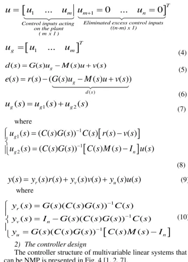
The controller structure of multivariable linear systems that can be NMP is presented in Fig. 4 [1, 2, 7].

Fig. 4. The controller structure

Where M(s) is the transfer matrix of the proposed model. It is of a (n n) dimension. K1 is a chosen square matrix of a

(n n) dimension and K2 is a gain matrix of a (n n)

dimension. e is the controller input vector of a dimension (n 1) and uc is the control input vector of a dimension

(n 1).

The gain matrix K2 is used to compensate the static errors,

and the gain matrix K1 is used to ensure the controller stability.

In fact, the first part of this proposed controller which represents the approximate inversion approach is shown in Fig. 5. In this case, the controller can be expressed by (11).

1 1 1

1 1 1

n

C( s ) ( I K M( s )) K ( K  M( s ))

Fig. 5. The approximate inversion (multivariable systems)

Where In is the identity matrix of a dimension n and K1 is

an invertible square matrix ensuring the stability of the controller. In order to simplify our study, K1 can be expressed

by (12) where a∈ℝ+.

K

1



a I

n ₍₁₂₎

If we choose a high value of a in (12), we obtain a small value of which allows to approximate (K1-1 + M(s))-1 with

M(s)-1. In this case, C(s) is approximately equal to the model expression inverse as follows.

C( s )

≃ 1

M ( s )

 (13)

Therefore, the system output vector expression given in (9) can be expressed by (14).

y s

( )

≃

y s r s

_r

( ) ( )



y s v s

_v

( ) ( )

(14)

The coefficients of the characteristic polynomial of the controller state matrix whose values depend on the value of a

in (12) must satisfy the Routh-Hurwitz criterion in order to ensure the controller stability. Since M(s) is stable, a suitable choice of the matrix K1 ensures the controller stability.

However, in the case of NMP systems, the adequate coefficient value of a cannot be chosen to be very high which can lead to the system accuracy degradation. In fact, in order to ensure the system accuracy, i.e., a zero static error, the controller static gain matrix C(0) must be very close to the inverse of the model static gain matrix M(0) as shown in (15), which is not possible in the case of a small value of a [2].

C( )

0

≃

M ( )

0

1 (15) In order to remedy this problem, the gain matrix K2

presented in Fig. 4 is added. It allows to compensate the system static errors thanks to its expression given by (16) and ensures that C(s)M(s) = In.

1 1

2 1 n 1

0

0

K



K ( I





K M( ))M( )



(16)

The general controller expression for NMP multivariable systems is therefore presented by (17) as follows [2].

C( s )



K ( I

_{2 n}



K M( s )) K

₁ 1 ₁ (17)

III. ILLUSTRATIVE EXAMPLES

Two set-point signals r1 and r2 of type steps having an

amplitude equal to 1 are applied to the following two examples, such that r = [r1 r2]T. Nominal cases are considered,

i.e., systems with no external disturbances.

A. The case of a linear MP underactuated system

Considering the following linear MP underactuated system with one control input u1 and two outputs y1and y2. The system

transfer matrix G(s) is given by (18).

1 2 2 2 2 3 2 1

4 3 1

G s s s G(s) s G s s         _{ }            _{ }   

    ₍₁₈₎

The model transfer matrix M(s) is of a dimension (2 x 2) as explained previously. The system and the model outputs are expressed respectively by (19) and (20).



1 2



1

T

g

y y G u G u

(19)

1 11 12 1

21 22

2 2

The Model M The control input vector u

0

m

m

y

M

M

u

Mu

M

M

y

u















_

_









_





 







(20)

The model transfer functions M11 and M21 are successively

chosen to be close to G1 and G2. We consider the case of a

perfect modeling, such that M11 is equal to G1 and M21 is equal

to G2. M12 and M22 are chosen as first order transfer functions

so that they ensure the invertibility conditions of the matrix M. The chosen model is expressed by the following transfer matrix

M(s).

2

2

2 1

3 2 2

1 3

4 3 2 4

s

s s s

M (s) s

s s s

    _{  }         _{  } 

  ₍₂₁₎

The application of the Routh–Hurwitz stability criterion allows to assess the necessary and sufficient condition of the controller stability. In the case of this system, we must choose

a> -0.72 such that K1 = a × I2. The proposed IMC design

presented in Fig. 2 is applied and the controller of Fig. 4 is used in order to ensure a greater accuracy.

In this study, two cases are considered. In the first case, the gain matrix K1 is chosen to be equal to 1× I2 (a = 1), and in the

second case, K1 is equal to 40 × I2 (a = 40).

The gain matrix K2 which is relative to K1 = 1 × I2 is given

by (22).

2

2 5 1 1 3

. K    _



  ₍₂₂₎

The gain matrix K2 which is relative to K1 = 40 × I2 is given

by (23).

2

1 0375 0 0250

0 0250 1 0500

. . K . .     _ 

Fig. 6 and Fig. 7 show the system control inputs evolution in the cases where a = 1 and a = 40, respectively.

Fig. 8 and Fig. 9 show the system outputs signals in the cases where a = 1 and a = 40, respectively.

Fig. 6. Control inputs (linear MP underactuated system, case of a = 1)

Fig. 7. Control inputs ( linear MP underactuated system, case of a = 40)

Fig. 8. System outputs ( linear MP underactuated system, case of a =1)

Fig. 9. System outputs (linear MP underactuated system, case of a =40)

It can be shown in Fig. 6 and Fig. 7 that the excess control input u2 is successfully eliminated. Simulation results also

show the effects of the choice of the coefficient a on the system behavior. The more the value of a increases, the more the system responses are fast and accurate. This is explained by the fact that the approximated inverse is closer to the real inverse of the model. However, we note a significant peak of the control input u1 which appears at the initial instants in Fig. 7

which is due to the high value of a. The more the value of a

increases, the more the peak is high. This is due to the fact that the system at boot acts as an open-loop system controlled by a control signal vector C(s) which is equal to a×r(s). The peak is then eliminated by the feedback effect.

The problem of the control input peak can be solved by the use of a saturation bloc that is added to the controller configuration as shown in Fig. 10 [1].

Fig. 10.Controller structure with a saturation bloc

The same linear MP underactuated system presented in (18) and the case where K1 = 40 are considered. The gain matrix K2

is presented in (23).

Fig. 11 shows the control input evolution after having applied the controller structure in Fig. 10. Maximum eligible values of the control input u1 must be equal to -10 and 10. It is

shown that u1 has not exceeded the landmarks. It is also noted

Fig. 11.Control inputs

The next example presents the case of a linear NMP underactuated system.

B. The case of linear NMP underactuated system

We present in this example one control input/two outputs NMP system. It is represented by the following transfer matrix

1 2

2

2

1 1 1

2 1

G s

s s G( s )

s

G s s

  

 

   _{ } 

   

  

 

 _{ }   

   

(24)

where the unstable zero of G(s) is equal to 1.

The case of a perfect modeling is considered. So, the transfer function M11 is chosen to be equal to G1 and M21 is

chosen to be equal to G2. M12 and M22 are chosen as first order

transfer functions with stable poles and zeros in order to simplify the calculations and avoid model inversion and controller stability problems.

The model M is presented by the transfer matrix given in as follows.

11 12

2

2

21 22

1

1

1

2

1

1

2

1

1

M

M

s

s

s

s

M ( s )

s

M

M

_s

_s

_s













 

_{ }

_









 







 

_



_





_

_{ }

_

_





₍₂₅₎

The model has one unstable zero (equal to 1) which may cause instability of the controller if we apply a direct inversion of the model. The controller structure described in Fig. 4 allows us to overcome this blocking problem. In fact, the application of the Routh–Hurwitz stability criterion on the controller characteristic polynomial whose coefficients depend on the value of a allows us to determine the necessary and sufficient condition of the controller stability which is found to be a < 0.87. In this case, the stabilizing value of a is small. So, the approximated inverse model is different from the real one which requires the addition of the gain matrix K2 expressed

in (16). In our case, the gain matrices K1 and K2 are

respectively equal to (26) and (27).

K

1



0 1

. I

2 ₍₂₆₎

2

21 10

20 21

K    _



  ₍₂₇₎

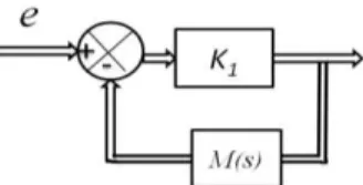
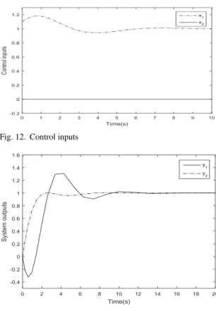
The control inputs and the system outputs are respectively presented in Fig. 12 and Fig. 13.

Simulation results prove the effectiveness of the approach to ensure a fast set-point tracking and to preserve the system performances in spite of the presence of underactuation and non-minimum phase behavior.

Fig. 12.Control inputs

Fig. 13.System outputs

In what follows, the implementation problems of the proposed IMC structure are discussed. Indeed, the influences of external disturbances, initial conditions and model parameters on the system behavior are studied.

IV. IMPLEMENTATION OF THE PROPOSED IMCSTRUCTURE

The linear underactuated system which is presented in (18) is considered in all the following examples and the controller structure of Fig. 4 is used. The chosen gain matrix K1 is equal

to 40×I and the reference signals are chosen to be steps of amplitude equal to 1.

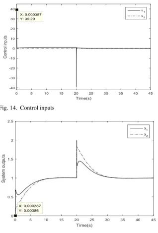
A. The case of disturbed system

In order to show a significant improvement of the accuracy and the disturbance rejection capability of the proposed IMC structure, we consider the case of a disturbed system where the disturbance signals v1 and v2 are chosen to be steps of

amplitude 1 that occurs at t = 20s as in (28).





20 20

1 2

T

s s

T e e

v(s) v v

s s

 

 

 _{  }

 

The case of a perfect modeling is considered. The model is expressed by its transfer matrix given by (21). The gain matrix

K2 is presented in (23).

Control inputs and system outputs are respectively presented in Fig. 14 and Fig. 15. Simulation results show that the IMC designed for linear underactuated systems guarantee an accurate set-point tracking and a fast disturbance rejection proving the robustness of the proposed approach.

Fig. 14.Control inputs

Fig. 15.System outputs

As we mentioned in the previous section, the control inputs peaks values can be reduced by the use of the controller structure with saturation bloc which was presented in Fig. 10.

B. The case of non-zero initial conditions

We consider the model presented in (21) and the gain matrix K2 given by (23).

The transfer matrix representation does not reveal the system evolution if it is not initially relaxed. So, we convert it into an equivalent state-space representation. This model and process representations are given respectively by (29) and (30) in a canonical form.

3 2 0 0

1 0 0 0

0 0 0 75 0 5

0 0 0 5 0

G A

. .

.  

 

 

 



   

 

 

2

0

1

0 G B

      

     

(29)

0.5 1 0 0 0 0 0.25 0.5

G

C   _

 

3 2 0 0 0 0

1 0 0 0 0 0

0 0 0 75 0 5 0 0

0 0 1 0 0 0

0 0 0 0 2 0

0 0 0 0 0 4

M

. .

A

 

 

 

 

   

  

 

 _ 

 

 _ 

 

2 0 0 0 0 5 0 0 0 0 1 0 2

M

. B

                  

(30)

0 5 1 0 0 1 0

0 0 0 5 0 5 0 1 5

M

. C

. . .

 

  

 

The disturbance vector presented in (28) is considered. We study these two examples of non-zero initial conditions of the system outputs:

0

y( t



s )

=[y01 y02]T =[0.75 0.375]T ;

0

y( t



s )

=[y01 y02]T =[1.530.675]T .

The resulting simulations are illustrated in Fig. 16 and Fig. 17 respectively. It can be shown that even for model and system initial conditions that may be non-zero and different, only the transient region of the output signals is affected which proves the robustness of the proposed control structure.

Fig. 16.System outputs

Fig. 17.System outputs

C. The case of imperfect modeling: model parameters effects

precise. Such model cannot provide a perfect description of the process behavior. Therefore, it can affect the process stability and/or precision which has led us to study the case of an imperfect model and test its parameter effects on the system evolution. These tests can help us to choose the model that best describes the controlled system and does not affect its stability.

The studied system is the linear underactuated system presented in (18). The gain matrix K2 is given by (23). We

present in the following the case of an imperfect modeling caused by the difference between the value of the process Damping Ratio (DR) and that of the model. We consider the model presented by the transfer matrix given by (31). The nominal case is studied.

The model and system DR values are denoted respectively as DRM and DRS.

11

2

1 2

1 3

4 3 2 4

M ( s ) s M ( s )

s

s s s

 

 _ 

  



 

 _{  } 

 

(31)

In the following tests, the DR value of the model transfer function (M11) is chosen to be very different from that of the

process (G1).

1) Test 1: DRM



DRS

In this case, the transfer matrix M11(s) is given by (32).

11 2

2

30 2

s M ( s )

s s

 

  (32) The system outputs are illustrated by Fig. 18. It can be shown that even for a high value of DRM, the system stability is maintained while the reference signal tracking becomes much slower.

Fig. 18.System outputs

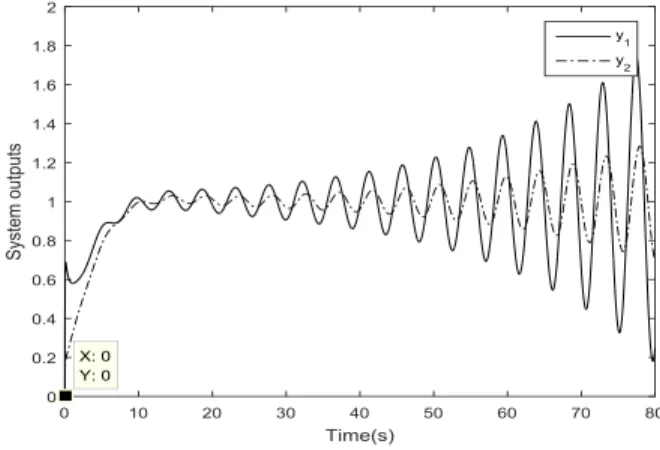
2) Test 2: DRM



DRS

The chosen transfer matrix M11(s) is given by (33).

₁₁

2

2

0 01 2

s M ( s )

s . s

 

  (33) The system outputs are presented in Fig. 19.

Fig. 19.System outputs

The obtained simulation results show that, in the case of a much smaller value of the DRM as compared to the DRS, the system becomes unstable.

In fact, the model response becomes much faster than that of the system. As a result, their outputs are added instead of being compared and the process behavior becomes equivalent to that of an open-loop system.

V. CONCLUSION

In this paper, a new approach to the IMC of continuous linear multivariable underactuated systems is presented. The realized research treats the case of underactuated MP and NMP systems.

Effects of non-zero initial conditions and model parameters on the system evolution are discussed.

Simulation results show the accuracy and the rapid disturbance rejection capability of the proposed IMC structure proving its robustness and its ability to remedy the problems caused by the system underactuation, the system NMP behavior, and non-zero initial conditions.

REFERENCES

[1] M. Naceur, “Sur la commande par modèle interne des systèmes

dynamiques continus et échantillonnés,” PhD dissertation, ENIT, Tunis, 2008.

[2] N. Touati, D. Soudani, M. Naceur and M. Benrejeb, “On the internal

model control of multivariable linear system,” International Conference

on Sciences and Techniques of Automatic control and computer engineering, STA, Sousse, 2011.

[3] M. Morari and E. Zafiriou , “RobustProcess Control,” Ed. Prentice Hall, Englewood cliffs, N.J., 1989.

[4] N. Touati, D. Soudani, M. Naceur and M. Benrejeb, “On an internal multimodel control for nonlinear multivariable system – A comparative

study,” International Journal of Advanced Computer Science and Applications, IJACSA,Vol. 4, No.7, 2013.

[5] M. Touzri, M. Naceur and D. Soudani, “A new design method of an Internal Multi-Model controller for a linear process with a variable time

delay,” International Conference on Control, Engineering & Information, CEIT, Sousse, 2013.

[7] M. Benrejeb, M. Naceur, D. Soudani, “On an internal model controller

based on the use of a specific inverse model,” International Conference

on Machine Intelligence, ACIDCA, Tozeur, 2005.

[8] C.E. Garcia and M. Morari, “Internal model control. l. A unifying review and some results,” Ind Eng.Chem. Process. Des,Vol.21, 1982. [9] A. Mezzi, D. Soudani and M. Benrejeb, “On the Internal Model Control

of Multivariable Linear Underactuated Systems,” Multi-Conference on

Computational Engineering in Systems Applications, CESA, Marrakech, 2015.

[10] A. Mezzi, and D. Soudani, “On the Internal Model Control of Multivariable Linear Underactuated Systems : Effects Of Initial

Conditions,” International Conference on Automation, Control,

Engineering and Computer Science, ACECS, Sousse, 2015.